A Modified Three-Term Conjugate Descent Derivative-Free Method for Constrained Nonlinear Monotone Equations and Signal Reconstruction Problems

Abstract

Iterative methods for solving constraint nonlinear monotone equations have been developed and improved by many researchers. The aim of this research is to present a modified three-term conjugate descent (TTCD) derivative-free method for constrained nonlinear monotone equations. The proposed algorithm requires low storage memory; therefore, it has the capability to solve large-scale nonlinear equations. The algorithm generates a descent and bounded search direction $d_k$ at every iteration independent of the line search. The method is shown to be globally convergent under monotonicity and Lipschitz continuity conditions. Numerical results show that the suggested method can serve as an alternative to find the approximate solutions of nonlinear monotone equations. Furthermore, the method is promising for the reconstruction of sparse signal problems.

1. Introduction

Consider the constrained nonlinear monotone equations of the following type:

$$P\left(x\right)=0,x\in G,$$

(1)

$G\subseteq {\mathbb{R}}^n$ is a closed, non-empty and convex set. $P:{\mathbb{R}}^n\to {\mathbb{R}}^n$ is monotone—that is,

$${(P\left(x\right)-P\left(y\right))}^T(x-y)\ge 0,\mathrm{for}\mathrm{all}x,y\in {\mathbb{R}}^n.$$

(2)

Problem (1) has drawn a lot of attention due to its applicability in many areas, such as power flow equations [1,2], financial forecasting problems [3], generalized proximal algorithms with Bregman distances [4], and economic equilibrium problems [5,6]. Furthermore, monotone variational inequality can be transformed into monotone nonlinear equations [7,8]. Numerous approaches such as Newton’s method, quasi-Newton’s method and many others—including the Levenberg–Marquardt method—are used to solve (1) [9,10,11] because of their fast convergence rate (see [12,13,14,15] for details). However, they require computing and storing of the inverse Jacobian matrix at every iteration, which is not always easy to compute or not available due to singularity. As such, many researchers have suggested derivative-free approaches that do not require computation of the Jacobian matrix; among others are [16,17,18,19,20,21,22,23,24,25]. A modified three-term conjugate descent (CD) derivative-free method is of interest in this research. The classical CD method was first presented by Fletcher [26], particularly for solving problems involving unconstrained optimization. Yan et al. [27] presented a globally convergent derivative-free method for solving large-scale nonlinear monotone equations with the projection method proposed in [28]. The numerical experiment reported illustrated that the methods are efficient. In [29], Koorapetse described a new three-term derivative-free method based on a projection approach to solve large-scale nonlinear monotone equations. Besides that, the search direction satisfies the sufficient descent condition and the method proved to be globally convergent. Abubakar et al. proposed a three-term derivative-free method in [30], where the Dai–Yuan type method, the Hestenes–Stiefel method, the Fletcher–Reeves method and the Polak–Ribiére–Polyak method were described as special cases. Jie and Zhong [31] modified the HS method for an unconstrained optimization problem. The global convergence of the algorithm was proved using the standard Wolfe line search. An interesting part of their research is that the search directions are always sufficiently descent independent of any line search and satisfy the conjugacy property as well. Motivated by the work of Jie and Zhong [31] and the fact that three-term derivative-free methods based on modified CD methods are rare in the literature, this paper considers a modified three-term, CD-type, derivative-free method to solve constrained nonlinear monotone equations and its application to sparse signal problems. The direction is sufficiently descent and bounded independent of the line search. The global convergence of the method is obtained under monotonicity and Lipschitz continuity conditions. Furthermore, a numerical experiment is provided to show the efficiency of the method by comparing with existing methods. The breakdown of the remaining parts of this article is as follows: The proposed algorithm and its derivation are given in Section 2. Section 3 provides the theoretical results. Section 4 presents the numerical experiments for the solution of nonlinear monotone equations. Sparse signal reconstruction is detailed in Section 5. Conclusions are made in Section 6. The norm of vectors is denoted by $\parallel ·\parallel$ and $P_k:=P\left(x_k\right).$ In addition, $H_{\mathcal{G}}[·]$ is the projection mapping from ${\mathrm{R}}^n$ onto $\mathcal{G}$ given by $H_{\mathcal{G}}\left[x\right]=argmin\{\parallel x-z\parallel :x\in {\mathrm{R}}^n,z\in \mathcal{G}\}$ for a non-empty, convex and closed set $\mathcal{G}\in {\mathrm{R}}^n$.

2. Algorithm and Its Derivation

In this part, we presented the framework of the algorithm and its derivation using a similar idea to that described in [31]. The proposed descent search direction is given by

$$d_k=\left\{\begin{array}{c}-P_{k}ifk=0\hfill \\ -P_k-\frac{P_k^T(P_k+d_{k-1})d_{k-1}}{{\lambda }_k}+\frac{\parallel P_k{\parallel }^2{d}_{k-1}}{{\lambda }_k},ifk\ge 1,\hfill \end{array}\right.$$

(3)

where

$${\lambda }_k=d_{k-1}^T{\widehat{P}}_{k-1},$$

(4)

$${\widehat{P}}_{k-1}=P_{k-1}+t_k{d}_{k-1},$$

(5)

$$t_k=1+max\left\{0,\frac{-d_{k-1}^T{P}_{k-1}}{\parallel d_{k-1}{\parallel }^2}\right\}.$$

(6)

Since the idea is obtained from an unconstrained optimization problem [31], to extend it to a system of constrained nonlinear monotone equations the following modification is needed.

Remark 1.

It is well known from the definition of ${\lambda }_k$ that

$$\begin{array}{cc}\hfill {\lambda }_k& = d_{k-1}^T{\widehat{P}}_{k-1},\hfill \\ \hfill & = d_{k-1}^T\left(P_{k-1}+t_k{d}_{k-1}\right)\hfill \\ \hfill & = d_{k-1}^T{P}_{k-1}+t_k{\parallel d_{k-1}\parallel }^2\hfill \\ & = d_{k-1}^T{P}_{k-1}+\left(1+max\left\{0,\frac{-d_{k-1}^T{P}_{k-1}}{\parallel d_{k-1}{\parallel }^2}\right\}\right){\parallel d_{k-1}\parallel }^2\hfill \\ & \ge d_{k-1}^T{P}_{k-1}+{\parallel d_{k-1}\parallel }^2-d_{k-1}^T{P}_{k-1}\hfill \\ \hfill & \ge \parallel d_{k-1}{\parallel }^2>0.\hfill \end{array}$$

Therefore, ${\lambda }_k>0$ whenever $d_{k-1}\ne 0.$

Thus, ${\lambda }_k$ is well defined.

The novel search direction $d_k$ always satisfies the sufficient descent property given by

$$P_k^T{d}_k\le -{\parallel P_k\parallel }^2.$$

(7)

3. Theoretical Results

This section presents the global convergence of the TTCD algorithm. However, before proceeding, the following conditions need to be provided.

Condition 1.

$G\subseteq {\mathbb{R}}^n$ is a closed, non-empty and convex set.

Condition 2.

P is L-Lipschitz continuous and monotone on ${\mathbb{R}}^n$, i.e.,

$${(P\left(x_1\right)-P\left(x_2\right))}^T(x_1-x_2)\ge 0,forall{x}_1,x_2\in {\mathbb{R}}^n$$

and

$$\parallel P\left(x_1\right)-P\left(x_2\right)\parallel \le L\parallel x_1-x_2\parallel ,L>0.$$

Lemma 1

([30]). If Conditions 1 and 2 hold, then  $\left\{x_k\right\}$ and $\left\{{\Gamma }_k\right\}$ are bounded. Furthermore,

$$\underset{k\to \infty }{lim}{v}_k\parallel d_k\parallel =0.$$

(8)

Remark 2.

Lemma 1 implies that there exists a non-negative σ such that $\parallel x_k\parallel \le \sigma$. Since $\left\{P_k\right\}$ is continuous and $\left\{x_k\right\}$ is bounded, then $\left\{P_k\right\}$ is also bounded. This implies that there is a positive constant M such that $\parallel P_k\parallel \le M$.

Lemma 2.

The search direction given by (3) is sufficiently descent.

Proof. 

When $k=0,$ then $P_0^T{d}_0\le -{\parallel P_0\parallel }^2.$ If $k\ge 1,$ then by (3) and (7), we have

$$\begin{array}{cc}\hfill P_k^T{d}_k& \le -\parallel P_k{\parallel }^2-\frac{P_k^T(P_k+d_{k-1})P_k^T{d}_{k-1}}{{\lambda }_k}+\frac{\parallel P_k{\parallel }^2{P}_k^T{d}_{k-1}}{{\lambda }_k},\hfill \\ \hfill & \le -\parallel P_k{\parallel }^2-\frac{\parallel P_k{\parallel }^2\left(P_k^T{d}_{k-1}\right)}{{\lambda }_k}-\frac{{\left(P_k^T{d}_{k-1}\right)}^2}{{\lambda }_k}+\frac{\parallel P_k{\parallel }^2\left(P_k^T{d}_{k-1}\right)}{{\lambda }_k},\hfill \\ \hfill & \le -\parallel P_k{\parallel }^2-\frac{{\left(P_k^T{d}_{k-1}\right)}^2}{{\lambda }_k},\hfill \\ & \le -\parallel P_k{\parallel }^2.\hfill \end{array}$$

This implies that the search direction obtained from (3) satisfies (7).    □

Lemma 3.

Assume that Conditions 1 and 2 hold. Let $\left\{{\zeta }_k\right\}$, $\left\{x_k\right\}$ and $\left\{d_k\right\}$ be defined by (28), (27) and (3), respectively; then, the following apply:

i. 

For all k, there exists a step-length $v_k=\mu {\rho }^i$, satisfying (26), for some

$i\in \mathbb{N}\cup \left\{0\right\}$, $k\ge 0.$

ii. 

The step-length $v_k$ satisfies the following relation:

$$v_k>min\left\{\mu ,\frac{\rho \parallel P_k{\parallel }^2}{(L+t)\parallel d_k{\parallel }^2}\right\}.$$

(9)

Proof. 

i. Assume to the contrary that there is a positive integer $k_0\ge 0$ such that (26) is not true for any integer $i\ge 0$—that is,

$$-P{(x_{k_0}+\mu {\rho }^i{d}_{k_0})}^T{d}_{k_0}<t\mu {\rho }^i{\parallel d_{k_0}\parallel }^2.$$

From the continuity of P and allowing $i\to \infty ,$ we have

$$-P{\left(x_{k_0}\right)}^T{d}_{k_0}\le 0.$$

(10)

However, from (7), we have

$$-P{\left(x_{k_0}\right)}^T{d}_{k_0}\le {\parallel P\left(x_{k_0}\right)\parallel }^2>0,$$

    which is a contradiction to (10). Hence, there exists $k_0\ge 0$ for which $v_k$ satisfies (26).

ii.

If $v_k\ne \mu ,$ then $v_k^{\prime }=\frac{v_k}{\rho }$ does not satisfy (26), which means

$$-P{(x_k+v_k^{\prime }{d}_k)}^T{d}_k<q{v}_k^{\prime }{\parallel d_k\parallel }^2.$$

(11)

By (7), we have

$$\parallel P_k{\parallel }^2=-P_k^T{d}_k={(P(x_k+v_k^{\prime }{d}_k)-P_k)}^T{d}_k-P{(x_k+v_k^{\prime }{d}_k)}^T{d}_k.$$

(12)

Substituting (11) into (12), by Lipschitz continuity of P and the Cauchy–Schwarz inequality, we have

$$\begin{array}{cc}\hfill \parallel P_k{\parallel }^2& < \parallel (P(x_k+v_k^{\prime }{d}_k)-P_k)\parallel \parallel d_k\parallel + q{v}_k^{\prime }{\parallel d_k\parallel }^2\hfill \\ \hfill & < L{v}_k^{\prime }\parallel d_k{\parallel }^2 + q{v}_k^{\prime }{\parallel d_k\parallel }^2\hfill \\ \hfill & = \left(L+q\right)v_k^{\prime }{\parallel d_k\parallel }^2.\hfill \end{array}$$

(13)

Substituting $v_k^{\prime }=v_k/\rho$ in (13), we have

$$v_k>\frac{\rho \parallel P_k{\parallel }^2}{\left(L+q\right){\parallel d_k\parallel }^2}.$$

Therefore, (9) is well established.

□

Theorem 1.

If Conditions 1 and 2 hold and $\left\{x_k\right\}$ is a sequence obtained from (27), then

$$\underset{k\to \infty }{lim\; inf}\parallel P_k\parallel =0.$$

(14)

However, the sequence $\left\{x_k\right\}$ converges to (1).

Proof. 

Suppose by contradiction that

$$\underset{k\to \infty }{lim\; inf}\parallel P_k\parallel \ne 0.$$

Then, there exists $m_1>0$ such that for all $k\ge 0,$

$$\parallel P_k\parallel \ge m_1.$$

(15)

By Cauchy–Schwarz inequality, from (7) and (15) for all $k\ge 0,$

$$\parallel d_k\parallel \ge \parallel P_k\parallel \ge m_1.$$

(16)

By Lemma (1), for all $k\ge 0$, $\left\{x_k\right\}$ and $\left\{P_k\right\}$ are bounded. We want to prove that $\left\{d_k\right\}$ given by (3) is bounded. For $k=0,$ we obtain

$$\parallel d_0\parallel = \parallel P_0\parallel \le M.$$

By (7), we can see that

$$P_0^T{d}_0\le -{\parallel P_0\parallel }^2.$$

(17)

From (3), if $k\ge 1,$ using Cauchy–Schwarz inequality and triangular inequality, we obtain

$$\begin{array}{cc}\hfill \parallel d_k\parallel & = \parallel -P_k-\frac{P_k^T(P_k+d_{k-1})d_{k-1}}{{\lambda }_k}+\frac{\parallel P_k{\parallel }^2{d}_{k-1}}{{\lambda }_k}\parallel ,\hfill \\ \hfill & \le \parallel P_k\parallel + \frac{\parallel P_k{\parallel }^2\parallel d_{k-1}\parallel }{\parallel d_{k-1}{\parallel }^2}+\frac{\left|P_k^T{d}_{k-1}\right|\parallel d_{k-1}\parallel }{\parallel d_{k-1}{\parallel }^2}+\frac{\parallel P_k{\parallel }^2\parallel d_{k-1}\parallel }{\parallel d_{k-1}{\parallel }^2},\hfill \\ \hfill & \le \parallel P_k\parallel + \frac{\parallel P_k{\parallel }^2}{\parallel d_{k-1}\parallel }+\parallel P_k\parallel +\frac{\parallel P_k{\parallel }^2}{\parallel d_{k-1}\parallel },\hfill \\ \hfill & \le 2\parallel P_k\parallel + \frac{2\parallel P_k{\parallel }^2}{\parallel d_{k-1}\parallel }.\hfill \end{array}$$

(18)

From Lemma (1), inequality (16) and Lipschitz continuity of P, relation (18) reduces to

$$\begin{array}{cc}\hfill \parallel d_k\parallel & \le 2M+\frac{2M^2}{m_1},\hfill \\ \hfill & \le 2M\left(1+\frac{M}{m_1}\right).\hfill \end{array}$$

(19)

Let $M^{*}=2M\left(1+\frac{M}{m_1}\right)$; then, we have

$$\parallel d_k\parallel \le M^{*},where{M}^{*}isapositiveconstant.$$

(20)

Multiply both sides (9) by $\parallel d_k\parallel$ to obtain

$$v_k\parallel d_k\parallel >min\left\{\mu \parallel d_k\parallel ,\frac{\rho \parallel P_k{\parallel }^2}{(L+t)\parallel d_k\parallel }\right\}\ge min\left\{\mu m_1,\frac{m_1^2\rho }{(L+t)M^{*}}\right\}>0.$$

(21)

Clearly, relation (21) above contradicts (8); therefore,

$$\underset{k\to \infty }{lim\; inf}\parallel P_k\parallel =0.$$

Since P is a continuous function and (14) holds, then $\left\{x_k\right\}$ has an accumulation point $\overline{x}$ at which $P\left(\overline{x}\right)=0$; this implies that $\overline{x}$ is a solution to (1). Since $\overline{x}$ is an accumulation point for $\left\{x_k\right\}$, then by Lemma (1), $\{\parallel x_k-\overline{x}\parallel \}$ converges. Therefore, it can be deduced that $\left\{x_k\right\}$ converges to $\overline{x}$.    □

4. Results for the Experiments

In this section, we present the results for the numerical experiments. We show the efficiency and effectiveness of the TTCD algorithm when it comes to solving nonlinear monotone equations by comparing with some existing methods using benchmark test problems. The experiments were run on a 4 GB RAM PC with a 2.13 GHz CPU. The following initial points and dimensions are considered:

• Five different initial points: $x_1={(0.1,0.1,\cdots ,0.1)}^T,x_2={(0.2,0.2,\cdots ,0.2)}^T,x_3={(0.5,0.5,\cdots ,0.5)}^T,x_4={(1.5,1.5,\cdots 1.5)}^T,x_5={(2,2,\cdots ,2)}^T$.
• Five different dimensions: $1000;5000;\mathrm{10,000};\mathrm{50,000};\mathrm{100,000}$.
• Eight problems (see Table 1 for details).

We choose the following as control parameters: $q=0.0001,\rho =0.8,\mu =1,\theta =1.2.$

The proposed algorithm is compared with MHS established by Yan et al. [27], MCDPM by Aji et al. [32] and PRPFR proposed by Yuan et al. [33]. $\parallel P_k\parallel \le {10}^{-5}$ is the stopping criteria for the iterations and $(-)$ stands for the failure of the method to solve the problem. The comparison of all the algorithms are based on the number of iteration (NOI), number of function evaluation (FEV) and CPU time (TIME).

Table 1. The test problems with their references are listed in the Table below.

S/N	Problem & Reference
1	Modified exponential function 2 [34]
2	Logarithmic function [34]
3	Problem 1 in [14]
4	Strictly convex function I [34]
5	Strictly convex function II [34]
6	Tridiagonal exponential function [35]
7	Nonsmooth function [36]
8	Problem 4 in [37]

Table 1. The test problems with their references are listed in the Table below.

S/N	Problem & Reference
1	Modified exponential function 2 [34]
2	Logarithmic function [34]
3	Problem 1 in [14]
4	Strictly convex function I [34]
5	Strictly convex function II [34]
6	Tridiagonal exponential function [35]
7	Nonsmooth function [36]
8	Problem 4 in [37]

The results for the experiments on the problems 1–8 in Table 1 are given in

Table 2. Numerical results for the problem with serial number 1 in Table 1.

		TTCD				PRPFR				MHS				MCDPM
Dimension	Initial Point	NOI	NFE	TIME	Norm	NOI	NFE	TIME	Norm	NOI	NFE	TIME	Norm	NOI	NFE	TIME	Norm
1000	$x_1$	1	7	0.39476	0	29	87	0.46498	9.59 × 10$-6$	7	22	0.26428	9.24 × 10$-6$	18	74	0.036251	8.83 × 10$-7$
	$x_2$	1	7	0.042189	0	31	94	0.14164	9.97 × 10$-6$	7	23	0.031263	7.02 × 10$-6$	9	38	0.021498	8.36 × 10$-7$
	$x_3$	1	7	0.017869	0	34	102	0.057707	9.84 × 10$-6$	7	22	0.017649	3.88 × 10$-6$	1	6	0.07097	0.00 × 10
	$x_4$	1	9	0.010377	0	31	93	0.058201	8.64 × 10$-6$	21	65	0.04509	6.29 × 10$-6$	1	6	0.050159	0.00 × 10
	$x_5$	1	10	0.010773	0	1	4	0.008098	0	1	6	0.008276	0	17	70	0.37822	7.83 × 10$-7$
5000	$x_1$	1	7	0.32858	0	28	85	4.3111	9.63 × 10$-6$	7	23	0.41693	9.97 × 10$-6$	17	69	0.6041	9.69 × 10$-7$
	$x_2$	1	7	0.25391	0	31	93	2.1436	8.42 × 10$-6$	8	26	0.18344	2.12 × 10$-6$	10	41	0.72735	9.79 × 10$-7$
	$x_3$	1	7	0.18581	0	33	100	1.0508	9.92 × 10$-6$	7	22	0.73022	7.23 × 10$-6$	1	6	0.1916	0.00 × 10
	$x_4$	1	9	0.1402	0	31	94	1.0252	9.95 × 10$-6$	22	68	0.91742	6.76 × 10$-6$	1	6	0.025797	0.00 × 10
	$x_5$	1	10	0.37567	0	1	4	0.31981	0	1	6	0.090721	0	17	70	0.15727	7.83 × 10$-7$
10,000	$x_1$	1	7	0.16721	0	28	84	3.1653	9.29 × 10$-6$	8	26	1.0706	1.92 × 10$-6$	16	66	0.67978	9.62 × 10$-7$
	$x_2$	1	7	0.22336	0	30	91	2.688	9.63 × 10$-6$	8	26	0.99103	2.99 × 10$-6$	10	42	0.59915	3.62 × 10$-7$
	$x_3$	1	7	0.18297	0	33	99	1.156	9.54 × 10$-6$	7	22	0.7447	9.96 × 10$-6$	1	6	0.36702	0.00 × 10
	$x_4$	1	9	0.18923	0	32	96	1.6268	8.56 × 10$-6$	22	68	1.813	9.55 × 10$-6$	1	6	0.24564	0.00 × 10
	$x_5$	1	10	0.44587	0	1	4	0.29106	0	1	6	0.13975	0	17	70	0.69621	7.83 × 10$-7$
50,000	$x_1$	1	7	0.26981	0	28	84	4.6798	7.80 × 10$-6$	8	26	1.2019	4.28 × 10$-6$	15	62	0.73916	8.85 × 10$-7$
	$x_2$	1	7	0.38483	0	30	90	3.8824	8.36 × 10$-6$	8	26	1.1829	6.68 × 10$-6$	10	42	0.87964	8.11 × 10$-7$
	$x_3$	1	7	0.33872	0	32	97	3.3427	9.79 × 10$-6$	8	26	1.3301	1.44 × 10$-6$	1	6	0.39671	0.00 × 10
	$x_4$	1	9	0.38542	0	33	99	3.6148	7.81 × 10$-6$	23	72	3.1315	8.72 × 10$-6$	1	6	0.44635	0.00 × 10
	$x_5$	1	10	0.37461	0	1	4	0.34298	0	1	6	0.23315	0	17	70	1.799	7.83 × 10$-7$
100,000	$x_1$	1	7	0.46499	0	27	82	4.8191	9.68 × 10$-6$	8	26	1.2872	6.06 × 10$-6$	15	61	1.2556	8.80 × 10$-7$
	$x_2$	1	7	0.4386	0	29	88	5.0801	9.95 × 10$-6$	8	26	1.0233	9.45 × 10$-6$	11	45	0.99889	5.96 × 10$-7$
	$x_3$	1	7	0.42428	0	32	96	5.153	9.54 × 10$-6$	8	26	1.2453	2.03 × 10$-6$	17	70	2.3563	7.83 × 10$-7$
	$x_4$	1	9	0.75986	0	33	99	4.7671	8.20 × 10$-6$	24	74	3.4883	7.01 × 10$-6$	15	61	2.5622	8.80 × 10$-7$
	$x_5$	1	10	0.82569	0	1	4	0.30469	0	1	6	0.44519	0	11	45	1.8746	5.96 × 10$-7$

,

Table 3. Numerical results for the problem with serial number 2 in Table 1.

		TTCD				PRPFR				MHS				MCDPM
Dimension	Initial Point	NOI	NFE	TIME	Norm	NOI	NFE	TIME	Norm	NOI	NFE	TIME	Norm	NOI	NFE	TIME	Norm
	$x_1$	5	17	0.04688	2.69 × ${10}^{-6}$	41	122	0.09586	8.12 × ${10}^{-6}$	10	29	0.02615	6.78 × ${10}^{-6}$	8	23	0.02071	8.24 × ${10}^{-6}$
1000	$x_1$	5	17	0.0957	2.69 × 10$-6$	41	122	0.086591	8.12 × 10$-6$	10	29	0.035475	6.78 × 10$-6$	8	23	0.020611	8.24 × 10$-7$
	$x_2$	5	17	0.018214	3.77 × 10$-6$	42	125	0.088716	8.01 × 10$-6$	10	29	0.02479	8.75 × 10$-6$	8	23	0.020254	6.96 × 10$-7$
	$x_3$	5	16	0.01802	2.52 × 10$-6$	35	104	0.07553	9.94 × 10$-6$	10	28	0.02561	4.63 × 10$-6$	8	24	0.025511	3.73 × 10$-7$
	$x_4$	5	16	0.017993	3.74 × 10$-6$	36	106	0.079168	8.80 × 10$-6$	10	28	0.026581	5.12 × 10$-6$	10	30	0.031719	4.77 × 10$-7$
	$x_5$	5	16	0.017177	4.40 × 10$-6$	41	120	0.080882	9.67 × 10$-6$	12	33	0.031571	4.69 × 10$-6$	10	30	0.025475	4.77 × 10$-7$
5000	$x_1$	5	17	0.051785	5.33 × 10$-6$	43	129	3.7411	9.94 × 10$-6$	11	32	1.4018	4.20 × 10$-6$	8	24	0.80266	3.29 × 10$-7$
	$x_2$	5	17	0.44454	7.48 × 10$-6$	44	132	1.2991	9.84 × 10$-6$	11	32	1.614	5.45 × 10$-6$	8	24	0.83206	2.91 × 10$-7$
	$x_3$	5	16	0.5018	4.77 × 10$-6$	38	112	1.12	9.91 × 10$-6$	10	28	0.73226	9.91 × 10$-6$	8	24	0.93838	3.52 × 10$-7$
	$x_4$	5	16	0.62636	6.82 × 10$-6$	39	116	3.0834	9.78 × 10$-6$	10	29	0.9578	9.47 × 10$-6$	11	32	1.0369	5.29 × 10$-7$
	$x_5$	5	16	0.67811	7.11 × 10$-6$	44	129	1.3612	9.31 × 10$-6$	12	34	1.2389	7.14 × 10$-6$	11	32	0.18547	5.29 × 10$-7$
10,000	$x_1$	3	9	0.31947	6.46 × 10$-6$	45	134	1.6464	8.54 × 10$-6$	11	32	0.97057	5.94 × 10$-6$	8	24	0.92705	4.58 × 10$-7$
	$x_2$	6	19	0.90193	1.78 × 10$-6$	46	137	2.6507	8.46 × 10$-6$	11	32	1.2003	7.69 × 10$-6$	8	24	0.99062	4.07 × 10$-7$
	$x_3$	5	16	0.74091	6.60 × 10$-6$	40	118	3.5742	8.06 × 10$-6$	10	29	1.286	9.76 × 10$-6$	8	24	1.0536	3.49 × 10$-7$
	$x_4$	5	16	0.35192	9.38 × 10$-6$	41	121	1.9318	8.57 × 10$-6$	11	31	1.126	5.46 × 10$-6$	11	32	1.1206	7.47 × 10$-7$
	$x_5$	5	16	0.6133	9.62 × 10$-6$	45	132	1.691	9.98 × 10$-6$	13	36	1.1217	4.03 × 10$-6$	11	32	1.1223	7.47 × 10$-7$
50,000	$x_1$	5	17	0.9371	4.25 × 10$-7$	48	143	6.2426	8.38 × 10$-6$	11	33	1.6664	9.28 × 10$-6$	9	26	1.3262	5.06 × 10$-7$
	$x_2$	6	19	0.86941	3.93 × 10$-6$	49	146	4.7769	8.30 × 10$-6$	12	35	1.6582	4.81 × 10$-6$	8	24	1.3916	9.03 × 10$-7$
	$x_3$	5	17	1.075	4.28 × 10$-7$	42	125	4.8675	9.85 × 10$-6$	11	31	1.6966	8.69 × 10$-6$	8	24	1.26	3.47 × 10$-7$
	$x_4$	5	17	0.96344	6.06 × 10$-7$	44	130	4.2812	8.54 × 10$-6$	11	32	1.5693	8.67 × 10$-6$	11	33	1.8148	3.50 × 10$-7$
	$x_5$	5	17	1.0274	6.12 × 10$-7$	48	141	4.9917	9.78 × 10$-6$	13	36	2.0201	8.98 × 10$-6$	11	33	2.1212	3.50 × 10$-7$
100,000	$x_1$	5	17	1.289	5.99 × 10$-7$	49	146	6.8958	9.01 × 10$-6$	12	35	2.4472	5.25 × 10$-6$	9	26	1.9055	7.14 × 10$-7$
	$x_2$	6	19	1.3907	5.55 × 10$-6$	50	149	5.8892	8.92 × 10$-6$	12	35	2.4688	6.80 × 10$-6$	9	26	2.0498	6.38 × 10$-7$
	$x_3$	5	17	1.2553	6.03 × 10$-7$	44	130	5.987	8.47 × 10$-6$	11	32	2.5203	8.60 × 10$-6$	8	24	1.6286	3.47 × 10$-7$
	$x_4$	5	17	1.5648	8.53 × 10$-7$	45	133	6.2888	9.20 × 10$-6$	12	34	2.6034	4.91 × 10$-6$	11	33	2.7362	4.94 × 10$-7$
	$x_5$	5	17	1.7077	8.60 × 10$-7$	49	145	6.7405	9.98 × 10$-6$	13	37	2.6897	8.88 × 10$-6$	11	33	2.756	4.94 × 10$-7$

,

Table 4. Numerical results for the problem with serial number 3 in Table 1.

		TTCD				PRPFR				MHS				MCDPM
Dimension	Initial Point	NOI	NFE	TIME	Norm	NOI	NFE	TIME	Norm	NOI	NFE	TIME	Norm	NOI	NFE	TIME	Norm
1000	$x_1$	4	13	0.013892	7.77 × 10$-6$	47	141	0.092229	8.32 × 10$-6$	10	31	0.023258	9.32 × 10$-6$	1	5	0.007193	0
	$x_2$	5	15	0.034216	2.72 × 10$-6$	49	147	0.089783	9.57 × 10$-6$	11	33	0.024557	7.35 × 10$-6$	1	5	0.007293	0
	$x_3$	4	12	0.013768	2.51 × 10$-6$	52	157	0.098241	9.73 × 10$-6$	12	36	0.029441	4.66 × 10$-6$	1	5	0.007014	0
	$x_4$	11	35	0.025443	6.74 × 10$-6$	56	168	0.10204	8.28 × 10$-6$	11	33	0.025179	7.77 × 10$-6$	1	5	0.006528	0
	$x_5$	11	35	0.02495	6.74 × 10$-6$	56	168	0.099741	8.28 × 10$-6$	13	39	0.033871	6.13 × 10$-6$	1	5	0.00867	0
5000	$x_1$	5	15	0.042458	3.48 × 10$-6$	50	150	4.4435	8.16 × 10$-6$	11	33	0.80606	8.34 × 10$-6$	1	5	0.17726	0
	$x_2$	5	15	0.04373	6.08 × 10$-6$	52	156	1.391	9.40 × 10$-6$	12	36	0.93636	4.60 × 10$-6$	1	5	0.14127	0
	$x_3$	4	12	0.10784	5.62 × 10$-6$	55	166	1.5696	9.55 × 10$-6$	12	37	1.4107	7.29 × 10$-6$	1	5	0.13105	0
	$x_4$	12	37	0.27214	5.43 × 10$-6$	59	177	1.3227	8.13 × 10$-6$	12	36	0.97416	4.87 × 10$-6$	1	5	0.24773	0
	$x_5$	12	37	0.13843	5.43 × 10$-6$	59	177	3.1086	8.13 × 10$-6$	13	40	0.99392	9.60 × 10$-6$	1	5	0.14151	0
10,000	$x_1$	5	15	0.21752	4.92 × 10$-6$	51	153	3.0496	8.77 × 10$-6$	11	34	1.017	8.26 × 10$-6$	1	5	0.15359	0
	$x_2$	5	15	0.10992	8.60 × 10$-6$	53	160	1.6167	9.59 × 10$-6$	12	36	0.9133	6.51 × 10$-6$	1	5	0.14256	0
	$x_3$	4	12	0.22389	7.95 × 10$-6$	57	171	3.9475	8.21 × 10$-6$	13	39	1.1891	4.12 × 10$-6$	1	5	0.12853	0
	$x_4$	12	37	0.20661	7.67 × 10$-6$	60	180	2.9248	8.73 × 10$-6$	12	36	1.3815	6.88 × 10$-6$	1	5	0.18035	0
	$x_5$	12	37	0.12426	7.67 × 10$-6$	60	180	2.337	8.73 × 10$-6$	14	42	0.85581	5.43 × 10$-6$	1	5	0.096199	0
50,000	$x_1$	5	16	0.40974	2.20 × 10$-6$	54	162	6.0399	8.61 × 10$-6$	12	36	0.96663	7.38 × 10$-6$	1	5	0.13193	0
	$x_2$	5	16	0.32448	3.85 × 10$-6$	56	168	5.0229	9.91 × 10$-6$	13	39	1.0361	4.08 × 10$-6$	1	5	0.22266	0
	$x_3$	4	13	0.2727	3.56 × 10$-6$	60	180	5.7702	8.06 × 10$-6$	13	39	1.3291	9.22 × 10$-6$	1	5	0.20316	0
	$x_4$	13	40	0.88417	3.98 × 10$-6$	63	189	5.8126	8.57 × 10$-6$	13	39	1.928	4.31 × 10$-6$	1	5	0.22315	0
	$x_5$	13	40	1.2791	3.98 × 10$-6$	63	189	5.6972	8.57 × 10$-6$	14	43	2.0536	8.50 × 10$-6$	1	5	0.18485	0
100,000	$x_1$	5	16	2.6019	3.11 × 10$-6$	55	165	7.2494	9.26 × 10$-6$	12	37	2.5901	7.31 × 10$-6$	1	5	0.30837	0
	$x_2$	5	16	0.50677	5.44 × 10$-6$	58	174	6.256	8.10 × 10$-6$	13	39	2.1932	5.77 × 10$-6$	1	5	0.2416	0
	$x_3$	4	13	0.82086	5.03 × 10$-6$	61	183	6.9018	8.66 × 10$-6$	13	40	2.0052	9.13 × 10$-6$	1	5	0.22573	0
	$x_4$	13	40	1.8095	5.63 × 10$-6$	64	192	7.3801	9.21 × 10$-6$	13	39	2.3259	6.10 × 10$-6$	1	5	0.29503	0
	$x_5$	13	40	1.6028	5.63 × 10$-6$	64	192	7.0349	9.21 × 10$-6$	15	45	2.8882	4.81 × 10$-6$	1	5	0.27045	0

,

Table 5. Numerical results for the problem with serial number 4 in Table 1.

		TTCD				PRPFR				MHS				MCDPM
Dimension	Initial Point	NOI	NFE	TIME	Norm	NOI	NFE	TIME	Norm	NOI	NFE	TIME	Norm	NOI	NFE	TIME	Norm
1000	$x_1$	1	2	0.014977	0	1	2	0.008553	0	1	2	0.008269	0	20	81	0.063565	9.90 × 10$-7$
	$x_2$	1	2	0.026176	0	1	2	0.008659	0	1	2	0.008284	0	1	3	0.00756	0
	$x_3$	1	2	0.010477	0	1	2	0.007917	0	1	2	0.009784	0	1	3	0.008726	0
	$x_4$	1	1	0.009676	0	1	4	0.008573	0	1	1	0.007314	0	9	26	0.028904	6.19 × 10$-7$
	$x_5$	1	1	0.009758	0	1	4	0.007923	0	1	1	0.007787	0	9	26	0.026248	6.19 × 10$-7$
5000	$x_1$	1	2	0.15403	0	1	2	0.24411	0	1	2	0.079542	0	22	88	2.2723	7.13 × 10$-7$
	$x_2$	1	2	0.0779	0	1	2	0.30731	0	1	2	0.093345	0	1	3	0.12692	0
	$x_3$	1	2	0.12547	0	1	2	0.25837	0	1	2	0.12491	0	1	3	0.092858	0
	$x_4$	1	1	0.022494	0	1	4	0.26094	0	1	1	0.017496	0	9	27	1.3101	2.76 × 10$-7$
	$x_5$	1	1	0.036342	0	1	4	0.35534	0	1	1	0.012998	0	9	27	1.0175	2.76 × 10$-7$
10,000	$x_1$	1	2	0.10049	0	1	2	0.27088	0	1	2	0.18825	0	22	89	1.3107	6.62 × 10$-7$
	$x_2$	1	2	0.14111	0	1	2	0.34003	0	1	2	0.11943	0	1	3	0.15195	0
	$x_3$	1	2	0.11487	0	1	2	0.56146	0	1	2	0.13215	0	1	3	0.13622	0
	$x_4$	1	1	0.031735	0	1	4	0.33398	0	1	1	0.017289	0	9	27	1.0115	3.91 × 10$-7$
	$x_5$	1	1	0.033518	0	1	4	0.40247	0	1	1	0.037098	0	9	27	1.1561	3.91 × 10$-7$
50,000	$x_1$	1	2	0.16977	0	1	2	0.43538	0	1	2	0.23996	0	23	93	4.2309	6.81 × 10$-7$
	$x_2$	1	2	0.23495	0	1	2	0.44127	0	1	2	0.17726	0	1	3	0.23854	0
	$x_3$	1	2	0.26851	0	1	2	0.29747	0	1	2	0.23986	0	1	3	0.14383	0
	$x_4$	1	1	0.06572	0	1	4	0.29184	0	1	1	0.056298	0	9	27	1.6538	8.74 × 10$-7$
	$x_5$	1	1	0.09506	0	1	4	0.46869	0	1	1	0.083448	0	9	27	1.5979	8.74 × 10$-7$
100,000	$x_1$	1	2	0.45274	0	1	2	0.54185	0	1	2	0.28671	0	23	93	5.6623	9.63 × 10$-7$
	$x_2$	1	2	0.33082	0	1	2	0.41999	0	1	2	0.31384	0	1	3	0.29981	0
	$x_3$	1	2	0.33148	0	1	2	0.43823	0	1	2	0.3507	0	1	3	0.24454	0
	$x_4$	1	1	0.14723	0	1	4	0.42649	0	1	1	0.15859	0	10	29	2.4583	6.18 × 10$-7$
	$x_5$	1	1	0.14368	0	1	4	0.46397	0	1	1	0.095907	0	10	29	2.7612	6.18 × 10$-7$

,

Table 6. Numerical results for the problem with serial number 5 in Table 1.

		TTCD				PRPFR				MHS				MCDPM
Dimension	Initial Point	NOI	NFE	TIME	Norm	NOI	NFE	TIME	Norm	NOI	NFE	TIME	Norm	NOI	NFE	TIME	Norm
1000	$x_1$	1	4	0.01906	0	46	139	0.076367	9.75 × 10$-6$	10	31	0.022036	7.77 × 10$-6$	21	85	0.13186	7.15 × 10$-7$
	$x_2$	1	4	0.010846	0	49	147	0.077697	8.44 × 10$-6$	11	33	0.022087	5.05 × 10$-6$	21	85	0.034548	7.15 × 10$-7$
	$x_3$	2	8	0.038847	0	51	154	0.078987	9.57 × 10$-6$	11	33	0.021167	4.15 × 10$-6$	1	6	0.016759	0.00 × 10
	$x_4$	1	7	0.014736	0	53	159	0.080936	9.18 × 10$-6$	1	5	0.007763	0	1	5	0.020092	0.00 × 10
	$x_5$	1	9	0.009923	0	52	156	0.080606	9.60 × 10$-6$	47	143	0.072079	9.29 × 10$-6$	1	5	0.013008	2.22 × 10$-16$
5000	$x_1$	1	4	0.10086	0	49	148	2.6231	9.57 × 10$-6$	11	33	0.4742	6.95 × 10$-6$	22	89	0.79118	7.38 × 10$-7$
	$x_2$	1	4	0.10232	0	52	156	2.9497	8.29 × 10$-6$	11	34	0.84249	7.90 × 10$-6$	22	89	0.6661	7.38 × 10$-7$
	$x_3$	2	8	0.27552	0	54	162	1.5443	9.89 × 10$-6$	11	33	1.1456	9.28 × 10$-6$	1	6	0.24211	0.00 × 10
	$x_4$	1	7	0.2915	0	56	168	2.6752	9.01 × 10$-6$	1	5	0.15603	0	1	5	0.026622	0.00 × 10
	$x_5$	1	9	0.21487	0	55	165	1.441	9.42 × 10$-6$	50	152	1.6409	8.44 × 10$-6$	1	5	0.07096	2.22 × 10$-16$
10,000	$x_1$	1	4	0.16575	0	51	153	3.1945	8.23 × 10$-6$	11	33	1.0745	9.83 × 10$-6$	23	92	0.20473	7.31 × 10$-7$
	$x_2$	1	4	0.1488	0	53	159	1.894	8.91 × 10$-6$	12	36	0.61285	4.47 × 10$-6$	23	92	0.22369	7.31 × 10$-7$
	$x_3$	2	8	0.33583	0	56	168	1.7796	8.08 × 10$-6$	11	34	1.154	9.19 × 10$-6$	1	6	0.26087	0.00 × 10
	$x_4$	1	7	0.17316	0	57	171	3.7837	9.68 × 10$-6$	1	5	0.040828	0	1	5	0.054397	0.00 × 10
	$x_5$	1	9	0.27009	0	56	169	3.1847	9.62 × 10$-6$	51	155	1.9967	8.85 × 10$-6$	1	5	0.22579	2.22 × 10$-16$
50,000	$x_1$	1	4	0.19745	0	54	162	4.8643	8.08 × 10$-6$	12	36	1.2212	6.16 × 10$-6$	24	96	1.3266	7.52 × 10$-7$
	$x_2$	1	4	0.15177	0	56	168	4.4589	8.75 × 10$-6$	12	36	1.4127	9.99 × 10$-6$	24	96	0.98972	7.52 × 10$-7$
	$x_3$	2	8	0.38192	0	58	175	5.0083	9.91 × 10$-6$	12	36	1.6327	8.22 × 10$-6$	1	6	0.34723	0.00 × 10
	$x_4$	1	7	0.34086	0	60	180	4.9077	9.50 × 10$-6$	1	5	0.18248	0	1	5	0.093625	0.00 × 10
	$x_5$	1	9	0.37025	0	59	177	5.0955	9.94 × 10$-6$	54	164	5.3971	8.04 × 10$-6$	1	5	0.095985	2.22 × 10$-16$
100,000	$x_1$	1	4	0.37103	0	55	165	6.3816	8.68 × 10$-6$	12	36	1.6237	8.71 × 10$-6$	24	97	2.2859	6.99 × 10$-7$
	$x_2$	1	4	0.22823	0	57	171	5.7132	9.40 × 10$-6$	12	37	1.8371	9.89 × 10$-6$	24	97	1.6916	6.99 × 10$-7$
	$x_3$	2	8	0.54986	0	60	180	5.8032	8.52 × 10$-6$	12	37	2.0415	8.13 × 10$-6$	1	5	0.22741	2.22 × 10$-16$
	$x_4$	1	7	0.38999	0	61	184	6.7707	9.70 × 10$-6$	1	5	0.35288	0	24	97	4.0911	6.99 × 10$-7$
	$x_5$	1	9	0.54538	0	61	183	5.3886	8.12 × 10$-6$	55	167	7.2288	8.43 × 10$-6$	24	97	3.5739	6.99 × 10$-7$

,

Table 7. Numerical results for the problem with serial number 6 in Table 1.

		TTCD				PRPFR				MHS				MCDPM
Dimension	Initial Point	NOI	NFE	TIME	Norm	NOI	NFE	TIME	Norm	NOI	NFE	TIME	Norm	NOI	NFE	TIME	Norm
1000	$x_1$	20	61	0.10016	6.95 × 10$-6$	59	177	0.13948	8.09 × 10$-6$	—	—	—	—	28	113	0.061562	6.96 × 10$-7$
	$x_2$	20	61	0.044003	4.82 × 10$-6$	58	175	0.12307	9.72 × 10$-6$	—	—	—	—	1001	4007	2.1789	2.0736
	$x_3$	20	63	0.078728	6.21 × 10$-6$	58	174	0.15125	9.02 × 10$-6$	—	—	—	—	1001	4007	2.2257	2.2094
	$x_4$	26	84	0.095104	7.13 × 10$-6$	56	168	0.12881	8.57 × 10$-6$	28	85	0.057195	8.82 × 10$-6$	13	39	0.030615	3.53 × 10$-7$
	$x_5$	43	137	0.1255	9.23 × 10$-6$	54	162	0.12107	8.75 × 10$-6$	49	149	0.085025	8.88 × 10$-6$	39	156	0.078792	8.55 × 10$-7$
5000	$x_1$	23	72	1.8365	6.89 × 10$-6$	61	184	4.4772	9.93 × 10$-6$	467	1407	7.9621	9.99 × 10$-6$	1001	4012	15.1572	1.8695
	$x_2$	24	74	2.0428	7.36 × 10$-6$	61	184	1.6081	9.55 × 10$-6$	—	—	—	—	1001	4007	8.4921	5.2384
	$x_3$	22	68	0.90321	5.53 × 10$-6$	61	183	1.8118	8.86 × 10$-6$	—	—	—	—	1001	4007	5.5223	5.8303
	$x_4$	28	90	1.3633	6.81 × 10$-6$	59	177	1.9934	8.42 × 10$-6$	31	94	0.14181	8.73 × 10$-6$	16	48	0.55779	4.96 × 10$-7$
	$x_5$	31	94	0.14181	8.73 × 10$-6$	57	171	2.3279	8.60 × 10$-6$	54	164	0.93908	8.26 × 10$-6$	41	164	1.2763	9.01 × 10$-7$
10,000	$x_1$	24	75	0.1859	9.83 × 10$-6$	63	189	2.2762	8.54 × 10$-6$	—	—	—	—	1001	4012	17.0512	2.9693
	$x_2$	25	77	0.96436	5.38 × 10$-6$	63	189	2.4627	8.22 × 10$-6$	—	—	—	—	1001	4007	13.237	7.5161
	$x_3$	22	69	1.6272	8.21 × 10$-6$	62	186	2.2821	9.52 × 10$-6$	—	—	—	—	1001	4007	13.1732	8.3369
	$x_4$	29	93	2.7352	6.67 × 10$-6$	60	180	2.3916	9.05 × 10$-6$	32	98	0.25086	9.07 × 10$-6$	33	122	0.95242	8.42 × 10$-7$
	$x_5$	58	183	2.9637	9.49 × 10$-6$	58	174	2.8124	9.24 × 10$-6$	56	170	1.1133	8.88 × 10$-6$	42	168	1.9567	9.88 × 10$-7$
50,000	$x_1$	24	75	3.044	9.79 × 10$-6$	66	198	7.6742	8.38 × 10$-6$	83	249	7.2083	9.80 × 10$-6$	1001	4013	49.0995	2.3302
	$x_2$	75	234	9.3715	8.53 × 10$-6$	66	198	4.4765	8.06 × 10$-6$	—	—	—	—	1001	4007	46.1181	16.9985
	$x_3$	23	71	2.6601	4.91 × 10$-6$	65	195	5.5787	9.35 × 10$-6$	—	—	—	—	1001	4007	45.8501	18.8076
	$x_4$	31	99	3.4197	9.01 × 10$-6$	63	189	5.8094	8.89 × 10$-6$	35	107	1.2342	8.98 × 10$-6$	1001	4004	46.1648	1.9526
	$x_5$	78	244	8.8083	9.48 × 10$-6$	61	183	6.2206	9.07 × 10$-6$	61	185	3.6487	9.97 × 10$-6$	47	187	3.4618	8.88 × 10$-7$
100,000	$x_1$	25	77	3.8554	3.88 × 10$-6$	67	201	9.3143	9.01 × 10$-6$	86	257	9.9301	8.88 × 10$-6$	1001	4013	89.2803	5.5249
	$x_2$	—	—	—	—	67	201	8.4452	8.67 × 10$-6$	658	1980	48.1837	9.99 × 10$-6$	1001	4007	87.5767	24.0734
	$x_3$	23	71	1.6217	6.80 × 10$-6$	66	199	8.0706	9.54 × 10$-6$	—	—	—	—	1001	4007	87.0774	26.6312
	$x_4$	32	102	3.5771	9.87 × 10$-6$	64	192	8.1187	9.55 × 10$-6$	37	112	2.5342	6.74 × 10$-6$	1001	4004	87.3123	2.9699
	$x_5$	76	239	10.7224	9.84 × 10$-6$	62	186	7.8989	9.75 × 10$-6$	64	194	6.2405	8.21 × 10$-6$	49	196	6.0736	8.31 × 10$-7$

,

Table 8. Numerical results for the problem with serial number 7 in Table 1.

		TTCD				PRPFR				MHS				MCDPM
Dimension	Initial Point	NOI	NFE	TIME	Norm	NOI	NFE	TIME	Norm	NOI	NFE	TIME	Norm	NOI	NFE	TIME	Norm
1000	$x_1$	9	30	0.041724	3.51 × 10$-6$	7	18	0.053759	9.06 × 10$-6$	13	39	0.042277	7.68 × 10$-6$	21	85	0.056556	7.81 × 10$-7$
	$x_2$	9	30	0.032227	2.07 × 10$-6$	7	18	0.018074	9.06 × 10$-6$	13	39	0.036789	7.38 × 10$-6$	22	88	0.053854	8.33 × 10$-7$
	$x_3$	7	25	0.025897	3.53 × 10$-6$	7	18	0.017956	9.06 × 10$-6$	13	39	0.035082	6.50 × 10$-6$	22	88	0.056923	8.64 × 10$-7$
	$x_4$	7	24	0.035928	3.30 × 10$-6$	7	18	0.017267	9.06 × 10$-6$	12	37	0.045048	8.93 × 10$-6$	22	88	0.057559	7.12 × 10$-7$
	$x_5$	5	19	0.074749	5.32 × 10$-6$	7	18	0.01742	9.06 × 10$-6$	12	36	0.036863	7.52 × 10$-6$	22	88	0.06216	7.12 × 10$-7$
5000	$x_1$	6	21	0.073893	7.59 × 10$-6$	6	16	0.74203	6.77 × 10$-7$	14	42	1.5985	4.81 × 10$-6$	22	89	1.785	8.05 × 10$-7$
	$x_2$	6	21	0.067512	7.61 × 10$-6$	6	16	0.75625	6.77 × 10$-7$	14	42	1.399	4.63 × 10$-6$	23	92	1.668	8.58 × 10$-7$
	$x_3$	6	21	0.067476	7.57 × 10$-6$	6	16	1.1359	6.77 × 10$-7$	14	42	1.2057	4.08 × 10$-6$	23	92	0.96043	8.91 × 10$-7$
	$x_4$	6	21	0.071118	5.83 × 10$-6$	6	16	0.40613	6.77 × 10$-7$	13	39	0.80464	8.00 × 10$-6$	23	92	1.3392	7.33 × 10$-7$
	$x_5$	6	21	0.070343	3.94 × 10$-6$	6	16	0.78932	6.77 × 10$-7$	13	39	1.3359	4.72 × 10$-6$	23	92	1.7417	7.33 × 10$-7$
10,000	$x_1$	7	24	0.13363	3.32 × 10$-6$	7	19	0.78323	5.87 × 10$-6$	14	42	1.5384	6.81 × 10$-6$	23	92	1.7332	7.97 × 10$-7$
	$x_2$	7	24	0.14005	3.43 × 10$-6$	7	19	0.95083	5.87 × 10$-6$	14	42	1.5111	6.55 × 10$-6$	23	93	2.24	7.98 × 10$-7$
	$x_3$	6	21	0.11446	8.67 × 10$-6$	7	19	1.5381	5.87 × 10$-6$	14	42	1.4081	5.77 × 10$-6$	23	93	1.4625	8.28 × 10$-7$
	$x_4$	5	18	0.11136	9.31 × 10$-6$	7	19	1.0212	5.87 × 10$-6$	13	40	1.089	7.92 × 10$-6$	23	93	1.2064	6.81 × 10$-7$
	$x_5$	5	18	0.13666	6.22 × 10$-6$	7	19	1.6565	5.87 × 10$-6$	13	39	1.3239	6.67 × 10$-6$	23	93	0.54021	6.81 × 10$-7$
50,000	$x_1$	5	19	0.43768	2.43 × 10$-6$	12	35	1.442	8.08 × 10$-6$	15	45	1.7295	4.26 × 10$-6$	24	96	2.2795	8.19 × 10$-7$
	$x_2$	5	19	0.41969	2.39 × 10$-6$	12	35	2.4552	8.08 × 10$-6$	15	45	1.8359	4.10 × 10$-6$	24	97	2.9665	8.20 × 10$-7$
	$x_3$	5	19	0.42038	2.26 × 10$-6$	12	35	1.7098	8.08 × 10$-6$	14	43	1.892	9.03 × 10$-6$	24	97	2.8791	8.52 × 10$-7$
	$x_4$	5	18	0.40879	9.62 × 10$-6$	12	35	1.9967	8.08 × 10$-6$	14	42	2.2515	7.09 × 10$-6$	24	97	3.5014	7.01 × 10$-7$
	$x_5$	5	18	0.41376	5.67 × 10$-6$	12	35	2.3075	8.08 × 10$-6$	14	42	2.3739	4.18 × 10$-6$	24	97	3.3654	7.01 × 10$-7$
100,000	$x_1$	5	19	0.7687	2.76 × 10$-6$	18	55	3.6832	9.84 × 10$-6$	15	45	2.8995	6.03 × 10$-6$	24	97	4.8971	7.61 × 10$-7$
	$x_2$	5	19	1.0646	2.66 × 10$-6$	18	55	3.2224	9.84 × 10$-6$	15	45	2.8558	5.80 × 10$-6$	25	100	4.5997	8.12 × 10$-7$
	$x_3$	5	19	0.82346	2.35 × 10$-6$	18	55	3.1908	9.84 × 10$-6$	15	45	2.585	5.11 × 10$-6$	25	100	4.8136	8.43 × 10$-7$
	$x_4$	5	19	1.1497	1.31 × 10$-6$	18	55	3.2991	9.84 × 10$-6$	14	43	2.6058	7.01 × 10$-6$	24	97	4.8878	9.91 × 10$-7$
	$x_5$	5	18	0.7911	8.01 × 10$-6$	18	55	3.4264	9.84 × 10$-6$	14	42	2.7503	5.91 × 10$-6$	24	97	4.6876	9.91 × 10$-7$

and

Table 9. Numerical results for the problem with serial number 8 in Table 1.

		TTCD				PRPFR				MHS				MCDPM
Dimension	Initial Point	NOI	NFE	TIME	Norm	NOI	NFE	TIME	Norm	NOI	NFE	TIME	Norm	NOI	NFE	TIME	Norm
1000	$x_1$	7	26	0.038192	4.69 × 10$-6$	13	40	0.034355	8.78 × 10$-6$	10	31	0.026314	3.45 × 10$-6$	17	70	0.074282	8.77 × 10$-7$
	$x_2$	7	26	0.027651	4.12 × 10$-6$	13	39	0.025373	7.19 × 10$-6$	9	29	0.022346	7.25 × 10$-6$	11	46	0.025641	5.26 × 10$-7$
	$x_3$	6	23	0.017775	1.42 × 10$-6$	13	39	0.024113	6.85 × 10$-6$	7	23	0.018538	6.02 × 10$-6$	11	47	0.026905	3.38 × 10$-7$
	$x_4$	7	26	0.022134	5.98 × 10$-6$	15	45	0.026703	5.54 × 10$-6$	10	31	0.025627	8.05 × 10$-6$	12	51	0.02692	7.22 × 10$-7$
	$x_5$	8	28	0.020408	3.31 × 10$-6$	15	45	0.02498	7.95 × 10$-6$	10	30	0.024156	3.84 × 10$-6$	11	47	0.026337	8.31 × 10$-7$
5000	$x_1$	8	29	0.10079	1.45 × 10$-6$	14	42	1.8974	8.52 × 10$-6$	10	31	1.1397	7.72 × 10$-6$	11	46	1.0893	5.78 × 10$-7$
	$x_2$	7	26	0.062245	9.22 × 10$-6$	14	42	0.94525	5.16 × 10$-6$	10	31	0.96032	5.28 × 10$-6$	15	63	0.93147	5.24 × 10$-7$
	$x_3$	6	23	0.059951	3.18 × 10$-6$	14	42	1.1388	4.92 × 10$-6$	8	25	0.99529	4.39 × 10$-6$	12	51	0.8147	3.59 × 10$-7$
	$x_4$	8	29	0.06846	1.85 × 10$-6$	15	46	0.81809	9.15 × 10$-6$	11	34	1.1985	3.44 × 10$-6$	11	46	0.96572	6.44 × 10$-7$
	$x_5$	8	28	0.066197	7.40 × 10$-6$	16	48	1.1876	5.71 × 10$-6$	10	30	0.8707	8.60 × 10$-6$	11	46	0.95789	5.72 × 10$-7$
10,000	$x_1$	8	29	0.10914	2.06 × 10$-6$	14	43	0.87715	8.91 × 10$-6$	10	32	0.89477	6.40 × 10$-6$	12	50	0.97286	5.16 × 10$-7$
	$x_2$	8	29	0.12	1.81 × 10$-6$	14	42	1.2638	7.30 × 10$-6$	10	31	1.1462	7.47 × 10$-6$	14	58	1.1714	7.59 × 10$-7$
	$x_3$	6	23	0.1001	4.50 × 10$-6$	14	42	1.5877	6.96 × 10$-6$	8	25	0.37139	6.21 × 10$-6$	13	55	1.0799	4.13 × 10$-7$
	$x_4$	8	29	0.3701	2.62 × 10$-6$	16	48	1.922	5.62 × 10$-6$	11	34	1.0558	4.87 × 10$-6$	12	50	1.4228	7.62 × 10$-7$
	$x_5$	9	31	0.12085	1.45 × 10$-6$	16	48	1.4143	8.07 × 10$-6$	10	31	0.23049	7.13 × 10$-6$	12	50	1.106	5.76 × 10$-7$
50,000	$x_1$	8	29	0.49017	4.60 × 10$-6$	15	45	2.619	8.66 × 10$-6$	11	34	1.3596	4.67 × 10$-6$	12	51	1.8309	6.78 × 10$-7$
	$x_2$	8	29	0.45313	4.04 × 10$-6$	15	45	2.5553	5.24 × 10$-6$	10	32	1.3002	9.80 × 10$-6$	19	78	2.0413	9.64 × 10$-7$
	$x_3$	7	26	0.39436	1.39 × 10$-6$	15	45	2.1702	5.00 × 10$-6$	8	26	1.2699	8.14 × 10$-6$	16	67	1.8872	2.99 × 10$-7$
	$x_4$	8	29	0.43932	5.85 × 10$-6$	16	49	2.5299	9.30 × 10$-6$	11	35	1.8906	6.39 × 10$-6$	12	51	1.5517	7.17 × 10$-7$
	$x_5$	9	31	0.51474	3.24 × 10$-6$	17	51	1.6011	5.80 × 10$-6$	11	33	1.4739	5.20 × 10$-6$	12	50	1.858	6.12 × 10$-7$
100,000	$x_1$	8	29	0.86788	6.50 × 10$-6$	15	46	2.6286	9.05 × 10$-6$	11	34	2.2841	6.60 × 10$-6$	13	55	2.6612	4.51 × 10$-7$
	$x_2$	8	29	0.86763	5.71 × 10$-6$	15	45	2.8049	7.41 × 10$-6$	11	34	2.1174	4.52 × 10$-6$	13	55	2.8656	4.36 × 10$-7$
	$x_3$	7	26	0.76683	1.97 × 10$-6$	15	45	2.2822	7.07 × 10$-6$	9	28	2.0024	3.75 × 10$-6$	18	75	3.9286	2.65 × 10$-7$
	$x_4$	8	29	1.2493	8.28 × 10$-6$	17	51	3.2253	5.71 × 10$-6$	11	35	2.3621	9.03 × 10$-6$	16	66	3.2361	4.79 × 10$-7$
	$x_5$	9	31	0.9051	4.59 × 10$-6$	17	51	2.0118	8.20 × 10$-6$	11	33	2.3617	7.35 × 10$-6$	16	66	2.6618	4.97 × 10$-7$

, respectively.

We plotted Figure 1, Figure 2 and Figure 3 using the performance profiles proposed in [38]. The TTCD algorithm has the least NOI in almost 82% of the problems compared to PRPFR, MHS and MCDPM, which have $20\%,$$18\%$ and $30\%$, respectively, as shown in Figure 1. Moreover, in Figure 2, the TTCD algorithm also has the highest FEV in approximately $67\%$ of the problems against PRPFR, MHS and MCDPM with $19\%$, $18\%$ and $21\%$, respectively. Figure 3 shows that the TTCD algorithm has the lowest time to converge to the solution of (1) in $60\%$ of the problems compared to PRPFR, MHS and MCDPM with approximately $5\%$, $14\%$ and $24\%$, respectively. In reference to the results mentioned above, we can say that the TTCD algorithm is more effective and robust than MCDPM, MHS and PRPFR. Therefore, it can serve as an alternative to those.

5. Signal Reconstruction

The aim of this section is to show how the sparse signal is reconstructed effectively by our proposed algorithm. A highly important aspect of many researchers is to obtain an ill-conditioned linear system of equations with sparse solutions. Some of them are objective functions, which can be transformed into minimization problems by employing a sparse (${\mathsf{\ell }}_1$) regularization term and a quadratic (${\mathsf{\ell }}_2$) error term [18], i.e.,

$$\underset{x}{min}\frac{1}{2}{\parallel y-Vx\parallel }_2^2+\omega {\parallel x\parallel }_1,$$

(22)

where $x\in {\mathbb{R}}^n,$$\omega >0,$$y\in {\mathbb{R}}^k$ is an observation and $V\in {\mathbb{R}}^{k\times n}$ ($k<<n$) is a linear transformation. Problem (22) is an unconstrained optimization problem, the solution of which will lead to the exact recovery of a sparse signal. Various approaches have been applied for solving (22), see [18,39,40,41,42,43] for more details. Furthermore, the gradient projection method (GPA) introduced by Figueiredo et al. [41] is well known to many researchers. The following is how the method was generated: Given $x\in {\mathbb{R}}^n$, x is given by

$$x=b-h,b\ge 0,h\ge 0,$$

where $b_i={\left(x_i\right)}_{+}$, $h_i={(-x_i)}_{+}$ for all $i=1,2,\cdots ,n$, and ${(·)}_{+}=max\{0,·\}$. Using

${\parallel x\parallel }_1=e_n^{T}b+e_n^{T}h$, where $e_n=(1,1,\cdots ,1)\in {\mathbb{R}}^n$, problem (22) can be expressed as

$$\underset{b,h}{min}\frac{1}{2}{\parallel y-V(b-h)\parallel }_2^2+\omega e_n^{T}b+\omega e_n^{T}h,b\ge 0,h\ge 0,$$

(23)

Equation (23) is a bound-quadratic constrained problem and can be written as

$$\underset{z}{min}\frac{1}{2}{z}^{T}Dz+c^{T}z,\mathrm{such}\mathrm{that}z\ge 0,$$

(24)

where $z=\left(\begin{array}{c}b\\ h\end{array}\right)$,    $c=\omega e_{2n}+\left(\begin{array}{c}-u_1\\ u_1\end{array}\right)$,    $u_1=V^{T}y$ and    $D=\left(\begin{array}{cc}{V}^{T}V& -V^{T}V\\ -V^{T}V& V^{T}V\end{array}\right)$. Since (24) is a convex quadratic problem, a positive, semi-definite matrix of D exists. By Xiao et al. [44], (24) can be transformed to

$$F\left(z\right)=min\{z,Dz+c\}=0,$$

(25)

where the function F is a vector-valued function and the “min” is interpreted as a component-wise minimum. It was proved in References [44,45] that F(z) is continuous and monotone. Therefore, problem (22) can be converted into problem (1) and, thus, Algorithm 1 (TTCD) can be applied to solve it.

Algorithm 1: A modified three-term conjugate descent (TTCD) derivative-free algorithm

Input. Choose $x_0\in {\mathbb{R}}^n,\theta ,\rho ,\mu ,q>0$, Set $k=0$. Step 1. If $\parallel P\left(x_k\right)\parallel \le \epsilon$ then stop. Else, go to Step 2. Step 2. Compute $d_k$ using (3)–(6). Step 3. Compute the step-length $v_k=\mu {\rho }^i,$ where $i=0,1,···,$ is the least non-negative integer satisfying the following inequality: $$-P{(x_k+v_k{d}_k)}^T{d}_k\ge q{v}_k{\parallel d_k\parallel }^2.$$ (26) Step 4. Let ${\Gamma }_k=x_k+v_k{d}_k.$ If ${\Gamma }_k\in G$ and $\parallel P\left({\Gamma }_k\right)\parallel \le \epsilon ,$ terminate. Else, compute $$x_{k+1}:=H_G\left[x_k-\theta {\zeta }_{k}P\left({\Gamma }_k\right)\right],$$ (27)     where $${\zeta }_k:=\frac{P{\left({\Gamma }_k\right)}^T(x_k-{\Gamma }_k)}{\parallel P\left({\Gamma }_k\right){\parallel }^2}.$$ (28) Step 5. Set $k=k+1$, repeat from Step 1.

The TTCD method was compared with the PCG method by Liu et al. [46], and by Algorithms 2.1a and 2.1b presented in [47]. The major aim for the experiments is to reconstruct a sparse signal of length n from k observations. The successful recovered signal is obtained by the mean squared error (MSE). The MSE is defined by

$$MSE:=\frac{1}{n}{\parallel x_j-x_{*}\parallel }^2.$$

The original and the recovered signals are, respectively, $x_j$ and $x_{*}$. The experiment consists of elements with size $2^7,$ $n=2^{11}$ and $k=2^9$ chosen at random. The noise is distributed with a variance of ${10}^{-3}$ and MSE of 0. However, the matrix V in (22) is generated in MATLAB with a $\mathrm{randn}(k,n)$ tool. We defined the objective function by

$$f\left(x\right)=\frac{1}{2}{\parallel Vx-y\parallel }_2^2+\omega {\parallel x\parallel }_1.$$

The initial point and continuation approach run by each method are the same on parameter $\omega$, as proposed in [46], to compare both methods. The starting point given by $x_0=V^{T}y$ is used to implement all algorithms, where

$$\begin{array}{c}\hfill \frac{|f_i-f_{i-1}|}{|f_{i-1}|}<{10}^{-5},i=1,2,3,\dots \end{array}$$

is the stopping condition and $f_i$ is the function value at $x_i$.

From Figure 4, one can see that the TTCD algorithm was able to recover the noisy signal with 131 iterations in 2.31 s, PCG with 150 iterations in 2.72 s, Algorithm 2.1a with 176 iterations in 3.11 s and Algorithm 2.1b with 136 iterations in 2.41 s. However, Algorithm 2.1a has the least MSE, followed by TTCD, Algorithm 2.1b and PCG, respectively.

The results reported in Figure 4 can be found in

Table 10. Experimental findings regarding the signal recovery problems.

	TTCD			PCG			Algorithm 2.1a			Algorithm 2.1b
S/N	TIME	IT	MSE	TIME	IT	MSE	TIME	IT	MSE	TIME	IT	MSE
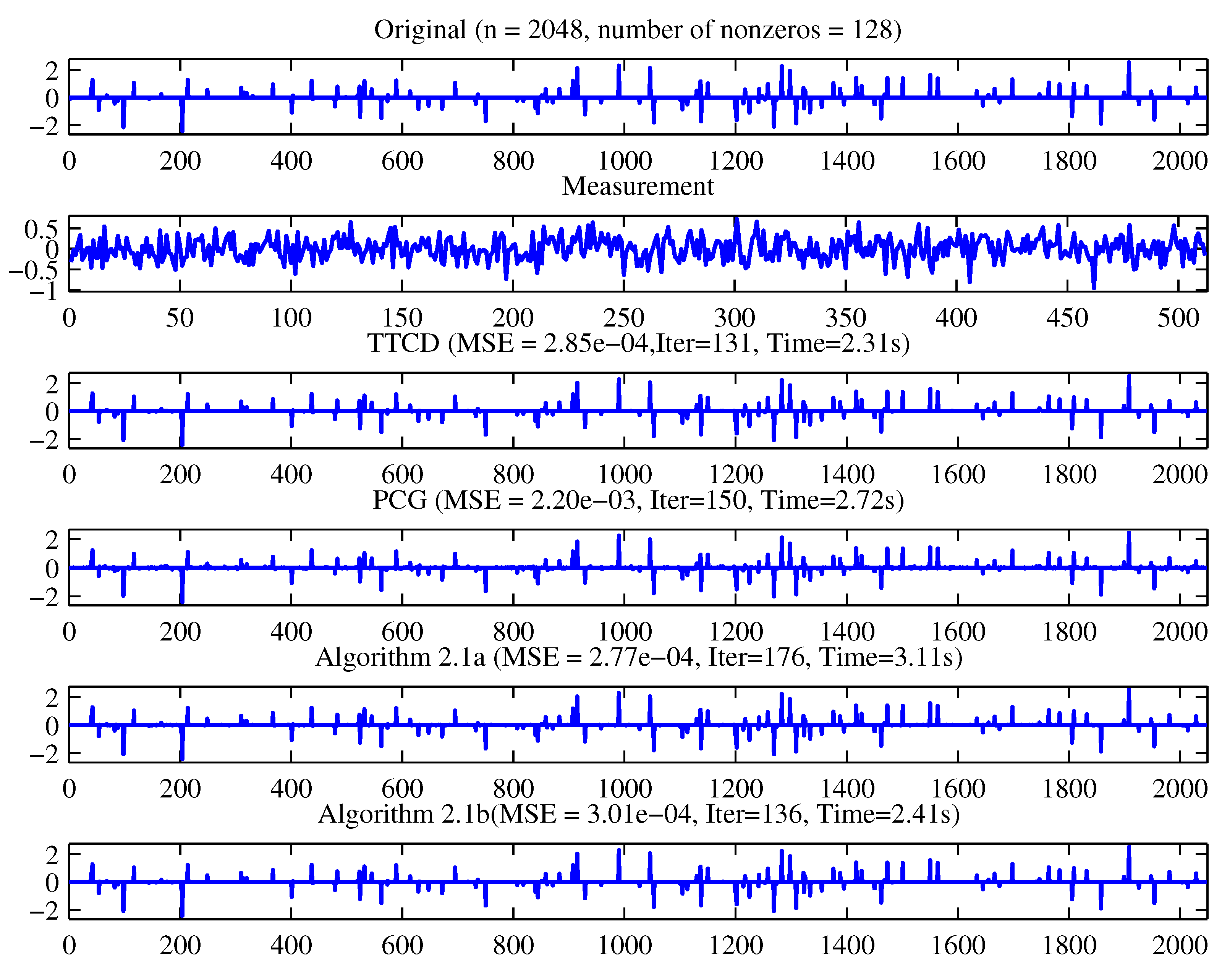
1	2.31	131	2.85 × 10$-4$	2.72	150	2.20 × 10$-3$	3.11	176	2.77 × 10$-4$	2.41	136	3.01 × 10$-4$
2	3.02	97	2.81 × 10$-5$	3.97	119	4.90 × 10$-5$	4.58	138	5.03 × 10$-5$	4.70	132	4.05 × 10$-5$
3	3.05	178	1.01 × 10$-5$	3.35	186	2.70 × 10$-5$	3.75	177	1.05 × 10$-5$	2.38	125	1.35 × 10$-5$
4	2.92	105	3.18 × 10$-5$	4.08	133	3.98 × 10$-5$	4.61	121	3.18 × 10$-5$	5.09	146	2.92 × 10$-5$
5	2.72	182	4.55 × 10$-3$	3.00	184	2.05 × 10$-3$	3.61	206	2.33 × 10$-3$	2.83	172	2.43 × 10$-3$
6	1.84	93	1.71 × 10$-3$	3.02	128	9.50 × 10$-4$	3.54	123	1.17 × 10$-3$	4.63	153	2.68 × 10$-3$
7	3.54	110	2.98 × 10$-5$	5.19	140	4.31 × 10$-5$	4.59	135	4.21 × 10$-5$	4.77	169	3.74 × 10$-5$
8	3.31	101	5.47 × 10$-5$	3.57	127	4.85 × 10$-3$	4.73	139	4.37 × 10$-3$	5.82	145	3.96 × 10$-3$
9	2.11	145	1.71 × 10$-3$	2.66	152	4.09 × 10$-3$	3.80	171	1.48 × 10$-3$	2.25	159	1.47 × 10$-3$
10	2.34	91	2.21 × 10$-5$	4.01	124	3.29 × 10$-5$	3.39	111	3.07 × 10$-5$	2.65	142	2.89 × 10$-5$
Average	2.716	123.3	8.432 × 10$-4$	3.557	144.3	1.433 × 10$-3$	3.971	149.7	9.792 × 10$-4$	3.753	147.9	1.099 × 10$-3$

, serial number 1.

Moreover, Figure 5 Shows the convergence properties of TTCD, PCG, Algorithm 2.1a and Algorithm 2.1b, respectively.

To ascertain the efficiency and the performance of the TTCD algorithm, the experiment was repeated up to 10 times by each algorithm and the average taken as shown in Table 10. On average, the TTCD recovered the noisy signal with the least number of iterations and CPU time. Furthermore, TTCD algorithm has the least MSE on average, followed by Algorithms 2.1a, Algorithms 2.1b and PCG, respectively. Hence, we can see TTCD as a better alternative to Algorithms 2.1a, Algorithms 2.1b and PCG, respectively, for solving signal reconstruction problems.

6. Conclusions

This research extended the unconstrained optimization problems to constrained nonlinear monotone equations by introducing a modified three-term CD derivative-free method using the projection method. The major advantage of the proposed method is that it does not require computation of the Jacobian matrix at each iteration or any linear equations; therefore, it is capable of solving large-scale constrained nonlinear monotone equations. Independent of the line search, the algorithm generates a bounded descent search direction. Under appropriate conditions, the method is shown to be globally convergent. Furthermore, the novel method is numerically robust and effective. Finally, the capacity of the method is tested to solve nonlinear equations equivalent to the ${\mathsf{\ell }}_1$-norm regularized minimization problems. The results obtained from the signal reconstruction experiments indicate that TTCD is faster than Algorithm 2.1a, Algorithm 2.1b and PCG, respectively. In addition, on average, TTCD has the least MSE compared to Algorithm 2.1a, Algorithm 2.1b and PCG, respectively.

References

- Wang, C.; Wang, Y. A superlinearly convergent projection method for constrained systems of nonlinear equations. J. Glob. Optim. 2009, 44, 283–296. [Google Scholar] [CrossRef]
- Chen, H.; Wang, Y.; Zhao, H. Finite convergence of a projected proximal point algorithm for the generalized variational inequalities. Oper. Res. Lett. 2012, 44, 303–305. [Google Scholar] [CrossRef]
- Dai, Z.; Dong, X.; Kang, J.; Hong, L. Forecasting stock market returns: New technical indicators and two-step economic constraint method. N. Am. J. Econ. Financ. 2020, 53, 101216. [Google Scholar] [CrossRef]
- Iusem, N.; Solodov, V. Newton-type methods with generalized distances for constrained optimization. Optimization 1997, 41, 257–278. [Google Scholar] [CrossRef]
- Dirkse, S.; Ferris, M. A collection of nonlinear mixed complementarity problems. Optim. Methods Softw. 1995, 5, 319–345. [Google Scholar] [CrossRef]
- Wang, Y.; Qi, L.; Luo, S.; Xu, Y. An alternative steepest direction method for the optimization in evaluating geometric discord. Pac. J. Optim. 2014, 10, 137–149. [Google Scholar]
- Fukushima, M. Equivalent differentiable optimization problems and descent methods for asymmetric variational inequality problems. Math. Program. 1992, 53, 99–110. [Google Scholar] [CrossRef]
- Zhao, Y.; Li, D. Monotonicity of fixed point and normal mappings associated with variational inequality and its application. SIAM J. Optim. 2001, 11, 962–973. [Google Scholar] [CrossRef]
- Dennis, J.E.; More, J.J. A characterization of superlinear convergence and its application to quasi-Newton methods. Math. Comput. 1974, 28, 549–560. [Google Scholar] [CrossRef]
- Dennis, E.J.J.; Moré, J.J. Quasi-Newton methods, motivation and theory. SIAM Rev. 1977, 19, 46–89. [Google Scholar] [CrossRef]
- Ioannis, K.A. On a nonsmooth version of Newton’s method using locally lipschitzian operators. Rend. Del Circ. Mat. Palermo 2007, 56, 5–16. [Google Scholar]
- Guanglu, Z.; Chuan, T.K. Superlinear convergence of a Newton-type algorithm for monotone equations. J. Optim. Theory Appl. 2005, 125, 205–221. [Google Scholar]
- Mohammad, H.; Waziri, M.Y. On Broyden-like update via some quadratures for solving nonlinear systems of equations. Turk. J. Math. 2015, 39, 335–345. [Google Scholar] [CrossRef]
- Zhou, W.J.; Li, H.D. A globally convergent BFGS method for nonlinear monotone equations without any merit functions. Math. Comput. 2008, 77, 2231–2240. [Google Scholar] [CrossRef]
- Donghui, L.; Fukushima, M. A globally and superlinearly convergent gauss–Newton-based BFGS method for symmetric nonlinear equations. SIAM J. Numer. Anal. 1999, 37, 152–172. [Google Scholar]
- Waziri, M.Y.; Yusuf, A.; Abubakar, A.B. Improved conjugate gradient method for nonlinear system of equations. Comput. Appl. Math. 2020, 39, 1–17. [Google Scholar] [CrossRef]
- Yusuf, A.; Adamu, A.K.; Lawal, L.; Ibrahim, A.K. A Hybrid Conjugate Gradient Algorithm for Nonlinear System of Equations through Conjugacy Condition. In Proceedings of the Artificial Intelligence and Applications, Wuhan, China, 18–20 November 2023. [Google Scholar]
- Abubakar, A.B.; Kumam, P.; Mohammad, H.; Awwal, A.M. An Efficient Conjugate Gradient Method for Convex Constrained Monotone Nonlinear Equations with Applications. Mathematics 2019, 7, 767. [Google Scholar] [CrossRef]
- Zhifeng, D.; Huan, Z. A modified Hestenes-Stiefel-type derivative-free method for large-scale nonlinear monotone equations. Mathematics 2020, 8, 168. [Google Scholar] [CrossRef]
- Awwal, A.M.; Ishaku, A.; Halilu, A.S.; Stanimirović, P.S.; Pakkaranang, N.; Panyanak, B. Descent Derivative-Free Method Involving Symmetric Rank-One Update for Solving Convex Constrained Nonlinear Monotone Equations and Application to Image Recovery. Symmetry 2022, 14, 2375. [Google Scholar] [CrossRef]
- Abubakar, A.B.; Kumam, P.; Awwal, A.M.; Thounthong, P. A modified self-adaptive conjugate gradient method for solving convex constrained monotone nonlinear equations for signal recovery problems. Mathematics 2019, 7, 693. [Google Scholar] [CrossRef]
- Sabi’u, J.; Muangchoo, K.; Shah, A.; Abubakar, A.B.; Jolaoso, L.O. A modified PRP-CG type derivative-free algorithm with optimal choices for solving large-scale nonlinear symmetric equations. Symmetry 2021, 13, 234. [Google Scholar] [CrossRef]
- Awwal, A.M.; Wang, L.; Kumam, P.; Mohammad, H.; Watthayu, W. A projection Hestenes–Stiefel method with spectral parameter for nonlinear monotone equations and signal processing. Math. Comput. Appl. 2020, 25, 27. [Google Scholar] [CrossRef]
- Sulaiman, I.M.; Awwal, A.M.; Malik, M.; Pakkaranang, N.; Panyanak, B. A derivative-free mzprp projection method for convex constrained nonlinear equations and its application in compressive sensing. Mathematics 2022, 10, 2884. [Google Scholar] [CrossRef]
- Sabi’u, J.; Aremu, K.O.; Althobaiti, A.; Shah, A. Scaled three-term conjugate gradient methods for solving monotone equations with application. Symmetry 2022, 14, 936. [Google Scholar] [CrossRef]
- Fletcher, R. Practical methods of optimization. In Unconstrained Optimization, 1st ed.; Wiley: New York, NY, USA, 1987; Volume 1. [Google Scholar]
- Yan, Q.R.; Peng, X.Z.; Li, D.H. A globally convergent derivative-free method for solving large-scale nonlinear monotone equations. J. Comput. Appl. Math. 2010, 234, 649–657. [Google Scholar] [CrossRef]
- Solodov, M.; Svaiter, B. A globally convergent inexact Newton method for systems of monotone equations. In Reformulation: Nonsmooth, Piecewise Smooth, Semismooth and Smoothing Methods; Springer: Berlin/Heidelberg, Germany, 1998; pp. 355–369. [Google Scholar]
- Koorapetse, M. A new three-term conjugate gradient-based projection method for solving large-scale nonlinear monotone equations. Math. Model. Anal. 2019, 24, 550–563. [Google Scholar] [CrossRef]
- Abubakar, A.B.; Kumam, P.; Ibrahim, A.H.; Chaipunya, P.; Rano, S.A. New hybrid three-term spectral-conjugate gradient method for finding solutions of nonlinear monotone operator equations with applications. Math. Comput. Simul. 2021, 201, 670–683. [Google Scholar] [CrossRef]
- Jie, G.; Zhong, W. A new three-term conjugate gradient algorithm with modified gradient-differences for solving unconstrained optimization problems. Methods 2023, 2, 12. [Google Scholar]
- Aji, S.; Kumam, P.; Siricharoen, P.; Abubakar, A.B.; Yahaya, M.M. A Modified Conjugate Descent Projection Method for Monotone Nonlinear Equations and Image Restoration. IEEE Access 2020, 8, 158656–158665. [Google Scholar] [CrossRef]
- Yuan, G.; Li, T.; Hu, W. A conjugate gradient algorithm for large-scale nonlinear equations and image restoration problems. Appl. Numer. Math. 2020, 147, 129–141. [Google Scholar] [CrossRef]
- La Cruz, W.; Martínez, J.; Raydan, M. Spectral residual method without gradient information for solving large-scale nonlinear systems of equations. Math. Comput. 2006, 75, 1429–1448. [Google Scholar] [CrossRef]
- Bing, Y.; Lin, G. An efficient implementation of Merrill’s method for sparse or partially separable systems of nonlinear equations. SIAM J. Optim. 1991, 1, 206–221. [Google Scholar] [CrossRef]
- Abubakar, A.B.; Kumam, P.; Mohammad, H. A note on the spectral gradient projection method for nonlinear monotone equations with applications. Comput. Appl. Math. 2020, 39, 129. [Google Scholar] [CrossRef]
- Ding, Y.; Xiao, Y.H.; Li, J. A class of conjugate gradient methods for convex constrained monotone equations. Optimization 2017, 66, 2309–2328. [Google Scholar] [CrossRef]
- Dolan, E.D.; Moré, J.J. Benchmarking optimization software with performance profiles. Math. Program. 2002, 91, 201–213. [Google Scholar] [CrossRef]
- Figueiredo, M.A.T.; Nowak, R.D. An EM algorithm for wavelet-based image restoration. IEEE Trans. Image Process. 2003, 12, 906–916. [Google Scholar] [CrossRef]
- Beck, A.; Teboulle, M. A fast iterative shrinkage-thresholding algorithm for linear inverse problems. SIAM J. Imaging Sci. 2009, 2, 183–202. [Google Scholar] [CrossRef]
- Figueiredo, M.A.T.; Nowak, R.D.; Wright, S.J. Gradient projection for sparse reconstruction: Application to compressed sensing and other inverse problems. IEEE J. Sel. Top. Signal Process. 2007, 1, 586–597. [Google Scholar] [CrossRef]
- Van Den Berg, E.; Friedlander, M.P. Probing the Pareto frontier for basis pursuit solutions. SIAM J. Sci. Comput. 2008, 31, 890–912. [Google Scholar] [CrossRef]
- Birgin, E.G.; Martínez, J.M.; Raydan, M. Nonmonotone spectral projected gradient methods on convex sets. SIAM J. Optim. 2000, 10, 1196–1211. [Google Scholar] [CrossRef]
- Xiao, Y.; Wang, Q.; Hu, Q. Non-smooth equations based method for ℓ1-norm problems with applications to compressed sensing. Nonlinear Anal. Theory Methods Appl. 2011, 74, 3570–3577. [Google Scholar] [CrossRef]
- Pang, J.S. Inexact Newton methods for the nonlinear complementarity problem. Math. Program. 1986, 36, 54–71. [Google Scholar] [CrossRef]
- Liu, J.K.; Li, S.J. A projection method for convex constrained monotone nonlinear equations with applications. Comput. Math. Appl. 2015, 70, 2442–2453. [Google Scholar] [CrossRef]
- Gao, P.; He, C.; Liu, Y. An adaptive family of projection methods for constrained monotone nonlinear equations with applications. Appl. Math. Comput. 2019, 359, 1–16. [Google Scholar] [CrossRef]