Dynamics of Hepatitis B Virus Transmission with a Lévy Process and Vaccination Effects

Abstract

This work proposes a novel stochastic model describing the propagation dynamics of the hepatitis B virus. The model takes into account numerous disease characteristics, and environmental disturbances were collected using Lévy jumps and the conventional Brownian motions. Initially, the deterministic model is developed, and the asymptotic behavior of the model’s solution near the equilibria is examined. The deterministic model is transformed into a stochastic model while retaining the Lévy jumps and conventional Brownian motions. Under specific assumptions, the stochastic system is shown to have a unique solution. The study further investigates the conditions that ensure the extinction and persistence of the infection. The numerical solutions to both stochastic and deterministic systems were obtained using the well-known Milstein and RK4 techniques, and the analytical findings are theoretically confirmed. The simulation suggests that the noise intensities have a direct relationship with the amplitudes of the stochastic curves around the equilibria of the deterministic system. Smaller values of the intensities imply negligible fluctuations of trajectories around the equilibria and, hence, better describe the extinction and persistence of the infection. It has also been found that both Brownian motions and the Lévy jump had a significant influence on the oscillations of these curves. A discussion of the findings of the study reveals other important aspects as well as some future research guidelines. In short, this study proposes a novel stochastic model to describe the propagation dynamics of the hepatitis B virus.

1. Introduction

Hepatitis B is a growing concern for scientists and healthcare professionals aiming to control the disease. Vaccines are an important tool in the fight against hepatitis B, helping to reduce the number of cases and the risk of serious complications. Vaccines are an important part of any public health strategy. It is worth mentioning that the administration of drugs and vaccines has successfully controlled numerous infectious diseases, including measles, typhoid, HBV, malaria, and COVID-19 [1,2,3]. Two decades earlier, the World Health Organization declared HBV infection a pandemic disease, and further investigation revealed that the infection is highly non-exposed and dangerous if not properly treated. Despite medications and the implementation of vaccines, approximately $0.37$ percent of core Pakistanis suffer from chronic HBV infection [4]. The infection and, consequently, death rates due to HBV are much lower in countries where proper vaccination programs are implemented at regular intervals. Vaccination programs for children are very effective and can significantly lower illness rates [5].

Various temporal and dynamical problems could be successfully dealt with via mathematical formalism; hence, better predictions and conclusions about the underlying system may be obtained. The dynamic behaviors of a nonlinear ODE system can always be projected in terms of their stable states (equilibria). The fundamental characteristics of non-constant statistical mechanics have a close relation with the mean lifetime of metastable nodes [6,7]. It is also possible that the dynamics of a real system could be affected by some external agents whose behaviors are very difficult to capture. However, some of the external impacts (specifically related to the environment), like random-driven forces and energy, can be captured mathematically by noises. These noises have a potential impact on the dynamic behaviors of the underlying system and, thus, their theoretical analysis in relation to equilibrium states is one of the burning research issues in epidemiology as well as in physics [8,9]. In particular, a natural system with metastable characteristics can deal with nonlinear relaxation behavior and its mean lifetime. Metastability is a prevalent behavior in physics and numerous other scientific domains such as biology, chemistry, and the study of high energy [10,11].

The literature on dynamical systems is rich, encompassing models using various techniques such as deterministic and stochastic approaches, fractional and fractal–fractional methods, etc. For experimentally testing a real scenario, the use of SDEs yields different outputs each time. For a better understanding, it is necessary to simulate the model thousands of times and then choose the average results. Similar to fractional models, it is also possible to analyze stochastic models for dynamical aspects, such as the existence of positive solutions, optimality, stability, and simulations. For more details, the authors are advised to see references [12,13,14,15] and the references cited therein.

Deterministic systems can be easily extended to stochastic models by incorporating noise, and these noises play an important role in describing real systems. Among other known noises, a Lévy noise is one of the most significant disturbances as it acts as a threshold parameter by drifting the velocity. In particular, the inclusion of this noise in epidemic models produces solid information and explains the hidden insights into the dynamic aspects of the disease. This is possible only if one imposes the Lipschitz condition on the underlying system. Specifically, the Lévy noise has many advantages over Gaussian. The Gaussian noise is widely used in mathematical modeling; however, this creates ambiguity in the modeling [16,17,18,19,20,21,22]. Because jumping is included, which diffuses problems caused by Lévy noises, the model outperforms the generalized Lévy model in terms of neuron efficiency development. Thus, studying the existing literature, we can conclude that the Lévy noise is very beneficial for problems where the stability of the system varies with time [23,24]. Environmental noise not only influences population dynamics, but it also plays an important part in many multidisciplinary physics models; see [25,26]. Its significance extends across several scientific fields, emphasizing its multidimensional impact on complex systems.

The organization for the remaining paper is as follows: In Section 2, the HBV model is formulated by keeping in mind certain assumptions about the system and the importance of the Lévy noise. A few basic results on stochastic modeling are presented in Section 3. The positivity of the solution to the proposed model and its existence are addressed in Section 4. The behavior of the solution of the stochastic model near the disease-free equilibrium of the associated deterministic system is studied in Section 5. The study was further extended to examine the asymptotic behavior of the stochastic curves near the endemic fixed point of the ODE model; this is detailed in Section 6, which explains the persistence of the infection. In Section 7, both stochastic and deterministic systems are simulated, and graphical illustrations are provided to validate the theoretical results. A discussion of the results, a summary of the findings, and a presentation of future research directions are included in Section 8, which concludes our work.

2. Model Formulation

Based on the dynamic features of HBV, Murad et al. [27] formulated a stochastic epidemic model for the disease and presented a model analysis under the vaccination effect. In this work, we will extend the model presented in [27], focusing on partial immunity, the nonlinear incidence of the infection, and vaccination as a control compartment. To formulate the model, we will decompose the entire population into six compartments: the susceptibles $S\left(t\right)$, acute infections $I_1\left(t\right)$, chronically infected people $I_2\left(t\right)$, the hospitalized class $H\left(t\right)$, the immune group $R\left(t\right)$, and vaccinated individuals $V\left(t\right)$. The birth flux enters the susceptible population at a rate of $\Psi \Pi$. At the same time, susceptibles move to the infected compartment at rates of $\frac{{\beta }_{1}S\left(t\right)I_1\left(t\right)}{N}+\frac{{\beta }_{2}S\left(t\right)I_2\left(t\right)}{N}$, and vaccinated individuals with weak immune systems move to the infected compartment at rates of $\frac{{\beta }_{3}V\left(t\right)I_1\left(t\right)}{N}+\frac{{\beta }_{4}V\left(t\right)I_2\left(t\right)}{N}$. It is assumed that the vaccinated class loses its immunity at a rate of $\eta V\left(t\right)$ and, thus, returns to the susceptible compartment. The vaccination rate of the susceptible class is $\gamma$, and the natural death rate for all compartments is $\chi$. The hospitalization rate of the acute and chronic compartments is assumed to be ${\Psi }_i$ for $i=1,2,$ respectively. Likewise, ${\gamma }_i$ for $i=1,2,$ is the recovery rate of the chronically infected compartment and disease-related death in the concerned compartment. Based on these (and other) assumptions, we have the following system of equations, which describes the dynamics of the underlying infection:

$$\begin{array}{cc}\hfill dS\left(t\right)=& \left[\Psi \Pi -\frac{{\beta }_1{I}_1\left(t\right)S\left(t\right)}{N}-\frac{{\beta }_2{I}_2\left(t\right)S\left(t\right)}{N}+\eta V\left(t\right)-(\gamma +\chi )S\left(t\right)\right]dt+{\delta }_{1}S\left(t\right)d{B}_1\left(t\right),\hfill \\ \hfill d{I}_1\left(t\right)=& \left[\frac{{\beta }_{1}S\left(t\right)I_1\left(t\right)}{N}+\frac{{\beta }_{2}S\left(t\right)I_2\left(t\right)}{N}+\frac{{\beta }_{3}V\left(t\right)I_1\left(t\right)}{N}+\frac{{\beta }_4{I}_2\left(t\right)V\left(t\right)}{N}-({\alpha }_1+{\alpha }_2+{\Psi }_1+\chi )I_1\left(t\right)\right]dt\hfill \\ & +{\delta }_2{I}_1\left(t\right)d{B}_2\left(t\right),\hfill \\ \hfill d{I}_2\left(t\right)=& \left[{\alpha }_1{I}_1\left(t\right)-({\gamma }_1+{\Psi }_2+{\gamma }_2+\chi )I_2\left(t\right)\right]dt+{\delta }_3{I}_2\left(t\right)d{B}_3\left(t\right),\hfill \\ \hfill dH\left(t\right)=& [{\Psi }_1{I}_1\left(t\right)+{\Psi }_2{I}_2\left(t\right)-({\Psi }_3+{\Psi }_4+\chi )H\left(t\right)]dt+{\delta }_{4}H\left(t\right)d{B}_4\left(t\right),\hfill \\ \hfill dR\left(t\right)=& \left[{\gamma }_1{I}_2\left(t\right)+{\alpha }_2{I}_1\left(t\right)+{\Psi }_{3}H\left(t\right)-\chi R\left(t\right)\right]dt+{\delta }_{5}R\left(t\right)d{B}_5\left(t\right),\hfill \\ \hfill dV\left(t\right)=& \left[\Psi (1-\Pi )+\gamma S\left(t\right)-\frac{{\beta }_{3}V\left(t\right)I_1\left(t\right)}{N}-\frac{{\beta }_{4}V\left(t\right)I_2\left(t\right)}{N}-(\eta +\chi )V\left(t\right)\right]dt+{\delta }_{6}V\left(t\right)d{B}_6\left(t\right).\hfill \end{array}$$

(1)

Here, $B\left(t\right)=B_1\left(t\right),\cdots ,B_6\left(t\right)$ denotes the white noises, which are continuous and real-valued on a complete probability space $(\Omega ,F,P)$ with the filtration function ${F_t}_{\{t\ge 0\}}$ (these are increasing and right-continuous while containing $F_0$ at all $P-$null sets). For each noise, we associate a constant intensity ${\delta }_i>0$ for $i=1,2,\dots ,6$. An initial approximate to model Equation (1) is given by the following equations:

$$\begin{array}{cc}\hfill S\left(t\right)& ={\phi }_1\left(t\right),I_1\left(t\right)={\phi }_2\left(t\right),I_2\left(t\right)={\phi }_3\left(t\right),H\left(t\right)={\phi }_4\left(t\right),R\left(t\right)={\phi }_1\left(t\right),V\left(t\right)={\phi }_1\left(t\right),\hfill \\ & {\phi }_i\left(t\right)\ge 0,t\in [-\omega ,0],i=1,\dots ,6.\hfill \\ & ({\phi }_1,{\phi }_2,{\phi }_3,{\phi }_4,{\phi }_5,{\phi }_6)\in C.\hfill \end{array}$$

(2)

In the above, the notion $C([-\omega ,0];R_{+}^6)$ is a closed norm space from the space $[-\omega ,0]$ to $R_{+}^6$, where $R_{+}^6=\{x=(x_1,x_2,\dots ,x_6)\in R^6:0<x_i,i=1,2,\dots ,6\}$. For a biological justification, we must assume ${\phi }_i\left(0\right)>0$ for all possible values of i. The majority of the parameters involved in system (1) are described in the model assumptions; however, for a detailed explanation, see

Table 1. Explanation of the parameters of the model.

Symbol	Description of Symbol
$\Pi$	The birth flux into the susceptible class.
${\beta }_1$	Rate at which the infection spreads from the susceptible to the acute compartment.
${\beta }_2$	Frequency of infections from chronic to susceptible.
${\beta }_3$	Transfer rate of the virus from the acute class to the vaccinated.
${\beta }_4$	Transfer rate of the virus from the chronic class to the vaccinated.
$\eta$	Waning immunity rate of vaccines.
$\chi$	The natural death rate.
$\gamma$	Rate of vaccinations of the susceptibles.
${\gamma }_1$	Rate at which chronically infected persons recover.
${\gamma }_2$	Disease-related death rate in the chronic compartment.
${\alpha }_1$	Rate at which acute infections progress to the chronic stage.
${\alpha }_2$	Recovery rate of acute individuals.
$\Psi$	The rate at which newborn babies do not receive vaccines against the infection.
${\Psi }_1,{\Psi }_2$	Hospitalization rates for the acute and chronic populations, respectively.
${\Psi }_3,{\Psi }_4$	The recovery rate of hospitalized individuals and the mortality rate due to the infection, respectively.

.

As previously stated, due to the many properties of the Lévy noise, it may be preferred above other noises in any epidemic investigation. Therefore, to effectively control and prevent HBV, we intend to model the governing dynamics of the disease, keeping in mind the Lévy noise with vaccinations, subject to partial immunity and nonlinear incidence of the disease. Thus, the modified version of system (1) is given by the following $S{I}_1{I}_{2}HRV$- model:

$$\begin{array}{cc}\hfill dS\left(t\right)=& \left[\Psi \Pi -\frac{{\beta }_{1}S\left(t\right)I_1\left(t\right)}{N}-\frac{{\beta }_{2}S\left(t\right)I_2\left(t\right)}{N}-(\chi +\gamma )S\left(t\right)+\eta V\left(t\right)\right]dt\hfill \\ & +{\delta }_{1}S\left(t\right)d{B}_1\left(t\right)+{\int }_X{Z}_1\left(x\right)S\left(t^{-}\right)\tilde{N}(dt,dx),\hfill \\ \hfill d{I}_1\left(t\right)=& \left[\frac{{\beta }_{1}S\left(t\right)I_1\left(t\right)}{N}+\frac{{\beta }_{2}S\left(t\right)I_2\left(t\right)}{N}+\frac{{\beta }_{3}V\left(t\right)I_1\left(t\right)}{N}+\frac{{\beta }_{4}V\left(t\right)I_2\left(t\right)}{N}-({\alpha }_1+{\alpha }_2+{\Psi }_1+\chi )I_1\left(t\right)\right]dt\hfill \\ & +{\delta }_2{I}_1\left(t\right)d{B}_2\left(t\right)+{\int }_X{Z}_2\left(x\right)I_1\left(t^{-}\right)\tilde{N}(dt,dx),\hfill \\ \hfill d{I}_2\left(t\right)=& \left[{\alpha }_1{I}_1\left(t\right)-({\gamma }_1+{\Psi }_2+{\gamma }_2+\chi )I_2\left(t\right)\right]dt+{\delta }_3{I}_2\left(t\right)d{B}_3\left(t\right)+{\int }_X{Z}_3\left(x\right)I_2\left(t^{-}\right)\tilde{N}(dt,dx),\hfill \\ \hfill dH\left(t\right)=& [{\Psi }_1{I}_1\left(t\right)+{\Psi }_2{I}_2\left(t\right)-({\Psi }_3+{\Psi }_4+\chi )H\left(t\right)]dt+{\delta }_{4}H\left(t\right)d{B}_4\left(t\right)+{\int }_X{Z}_4\left(x\right)H\left(t^{-}\right)\tilde{N}(dt,dx),\hfill \\ \hfill dR\left(t\right)=& \left[{\gamma }_1{I}_2\left(t\right)+{\alpha }_2{I}_1\left(t\right)+{\Psi }_{3}H\left(t\right)-\chi R\left(t\right)\right]dt+{\delta }_{5}R\left(t\right)d{B}_5\left(t\right)+{\int }_X{Z}_5\left(x\right)R\left(t^{-}\right)\tilde{N}(dt,dx),\hfill \\ \hfill dV\left(t\right)=& \left[\Psi (1-\Pi )+\gamma S\left(t\right)-\frac{{\beta }_{3}V\left(t\right)I_1\left(t\right)}{N}-\frac{{\beta }_{4}V\left(t\right)I_2\left(t\right)}{N}-(\eta +\chi )V\left(t\right)\right]dt\hfill \\ & +{\delta }_{6}V\left(t\right)d{B}_6\left(t\right)+{\int }_X{Z}_6\left(x\right)V\left(t^{-}\right)\tilde{N}(dt,dx).\hfill \end{array}$$

(3)

Other parameters have the same meanings, whereas, the notation $\tilde{N}$ denotes the compensated Poisson random measure, defined as $\tilde{N}(dt,dx)=\tilde{N}(dt,dx)-v\left(dx\right)dt$. In this context, $\tilde{N}$ represents the Poisson random measure, and $v(.)$ signifies its intensity measure. The intensities of the jumps are denoted as $Z_i=\{1,2,3,4,5,6\}$ and characterize the impact of random jumps within the model.

Model (3) represents an innovative framework for investigating HBV infectious diseases. Beyond elucidating the intricate dynamics of disease transmission in the human population, it underscores the pivotal role of vaccination in curbing the disease’s spread. By integrating these elements, the system provides useful insights into the dynamics of HBV, shedding light on the effectiveness of vaccines in reducing susceptibility.

3. Preliminaries

This subsection encompasses fundamental findings that are essential for establishing the primary results of the article. Initially, we consider a complete probability space $(\Omega ,F,F_t\ge 0,P)$ with a filtration that adheres to standard conditions (specifically, right continuity and inclusion of all P-null sets in $F_0$). Concerning stochastic differential equations involving Lévy jumps, let $y\left(t\right)\in R^n$ represent a solution to the following stochastic equation:

$$dy\left(t\right)=F_1(y\left(t\right),t)dt+F_2(y\left(t\right),t)dW\left(t\right)+{\int }_X{F}_3(y\left(t^{-}\right),t,x)\tilde{N}(dt,dx),$$

(4)

Here, $F_1:R^n\times R_{+}\to R^n,F_2:R^n\times R_{+}\to R^{n\times d}$, and $F_3:R^n\times R_{+}\times X\to R^n$ represent measurable functions. However, over the interval $t\in [0,T],W(.)$ is a d-dimensional Brownian motion, $\tilde{N}(dt,dy)$ is a 1-dimensional compensated Poisson process, and $y\left(t^{-}\right)$ denotes the left limit of $y\left(t\right)$. Consequently, for any given function, $G\in C^{1,2}(R^n\times R_{+};R_{+})$, the operator, L, derived from the stochastic process (4) can be expressed as follows:

$$\begin{array}{c}\hfill LG(y,t)=G_t(y,t)+G_y(y,t)F_1(y,t)+\frac{1}{2}\left[F_2^T(y,t)G_{yy}(y,t)F_2(y,t)\right]\\ \hfill +{\int }_X[G(y+F_3(y,t,x),t)-G(y,t)-G_y(y,t)F_3(y,t,x)]v\left(dx\right),\end{array}$$

(5)

where $G_t=\frac{\partial G}{\partial t}$, $G_y=(\frac{\partial G}{\partial y_1},\frac{\partial G}{\partial y_2},\dots ,\frac{\partial G}{\partial y_n}),G_{yy}={\left(\frac{{\partial }^{2}G}{\partial y_i\partial y_j}\right)}_{n\times n}$. As a result, the representation of It$\breve{o}$’s formula with jumps [28] is as follows:

$$\begin{array}{c}\hfill dG(y,t)=LG(y,t)+G_y(y,t)F_2(y,t)dW\left(t\right)+\\ \hfill +{\int }_X[G(y+F_3(y,t,z),t)-G(y,t)\tilde{N}(dt,dx).\end{array}$$

(6)

Lemma 1 

(Lemma 5.1, [29]). Let $Y\in \mathbb{C}\left(\right[0,+\infty )\times \Omega ,(0,+\infty \left)\right)$. If there exist two positive constants, ${\varphi }_1$ and ${\varphi }_2$, such that $lny\left(t\right)\ge {\varphi }_1\left(t\right)-{\varphi }_2{\int }_0^{t}y\left(s\right)ds+Y\left(t\right),\forall t\ge 0$, where $Y\in \mathbb{C}\left(\right[0,+\infty )\times \Omega ,R)$ and ${lim}_{t\to \infty }inf〈y\left(t\right)〉\ge \frac{{\psi }_1}{{\psi }_2}$ a.s. (almost sure).

4. Model Analysis

In this part of the manuscript, we will establish the results for the existence of a positive global solution to system (3).

Existence and Uniqueness of the Model Solution

As system (3) biologically describes the problem of population dynamics, it demands a positive, global, and bounded solution. In this subsection, we intend to study the well-posedness of system (3), investigating these aspects of the system. Before proving our main result, we will state the following important assumptions:

Assumption 1. 

There exists $D_n>0$, for each $x\in X$, and $n\in N$, s.t. (such that) ${\int }_X\mid F_i(z,x)-F_j(\overline{z},x){\mid }^{2}v\left(dx\right)\le n\mid z-\overline{z}{\mid }^2$, for all $z,\overline{z}\in R^n$, and $\mid \overline{z}\mid \vee \mid z\mid \le n$, for $i,j\in N_1^6,$ and

$$\begin{array}{cc}\hfill F_1(z,x)& ={\delta }_1\left(x\right)S\left(t\right),\hfill \\ \hfill F_2(z,x)& ={\delta }_2\left(x\right)I_1\left(t\right),\hfill \\ \hfill F_3(z,x)& ={\delta }_3\left(x\right)I_2\left(t\right),\hfill \\ \hfill F_4(z,x)& ={\delta }_4\left(x\right)H\left(t\right),\hfill \\ \hfill F_5(z,x)& ={\delta }_5\left(x\right)R\left(t\right),\hfill \\ \hfill F_6(z,x)& ={\delta }_6\left(x\right)V\left(t\right).\hfill \end{array}$$

(7)

Assumption 2. 

For $x\in X,$ with $1-{\delta }_i\left(x\right)>0,$ there surely exists a positive real number $\mathbb{C}$, such that ${\int }_X{(ln(1-{\delta }_i\left(x\right)))}^{2}v\left(dx\right)<\mathbb{C},fori\in \{1,2\}.$

Theorem 1. 

Assume that Assumptions 1 and 2 are true. Then for any $Z\left(0\right)=\left\{(S,I_1,I_2,H,R,V)\left(0\right)\right\}\in R_{+}^6,$ model (3) has only one positive solution $Z\left(t\right)=\{S\left(t\right),I_1\left(t\right),I_2\left(t\right),H\left(t\right),R\left(t\right),V\left(t\right)\}$ that remains in $R_{+}^6$ with only one probability, a.s.

Proof. 

Keeping in mind Assumption 1 and with reference to the local Lipschitz continuity of the drift and diffusion coefficients, a unique local solution $Z\left(t\right)$ exists for any $Z\left(0\right)\in R_{+}^6$ over the interval $t\in [0,{\tau }_e)$, where ${\tau }_e$ denotes the explosion time. To establish the global nature of the solution, it suffices to demonstrate that ${\tau }_e=\infty$, almost surely. To this end, we assume ${\rho }_0\ge 1$ represents a sufficiently large integer, such that $[1/{\rho }_0,{\rho }_0]$ encompasses all components of $Z\left(0\right)$. Consequently, for any integer $\rho \ge {\rho }_0$, we can define the following stopping time:

$$\widehat{{\tau }_{\rho }}=inf\left\{t\in [0,{\tau }_e];S\left(t\right)\notin (\frac{1}{\rho },\rho ),I_1\left(t\right)\notin (\frac{1}{\rho },\rho ),I_2\left(t\right)\notin (\frac{1}{\rho },\rho ),H\left(t\right)\notin (\frac{1}{\rho },\rho ),R\left(t\right)\notin (\frac{1}{\rho },\rho ),V\left(t\right)\notin (\frac{1}{\rho },\rho )\right\},$$

(8)

where $\widehat{{\tau }_{\rho }}$ increases as $\rho \to \infty$, defining $\widehat{{\tau }_{\infty }}={lim}_{\rho \to \infty }\widehat{{\tau }_{\rho }}$. It is apparent that $\widehat{{\tau }_{\infty }}\le {\tau }_e$, almost surely. Furthermore, if $\widehat{{\tau }_{\infty }}=\infty$, it implies ${\tau }_e=\infty$ almost surely, demonstrating that the solution $Z\left(t\right)\in {\mathbb{R}}_{+}^6$ for all $t\ge 0$. To conclude the proof, we aim to establish $\widehat{{\tau }_{\infty }}=\infty$, almost surely. Assuming the contrary, there exist constants $0<ϵ<1$ and $\overline{T}>0$ in such a way that $P\{\overline{T}\ge \widehat{{\tau }_{\infty }}\}>ϵ$.

Now, before moving further, we need to define the function given as follows:

$$\begin{array}{cc}\hfill G(S,I_1,I_2,H,R,V)& =S+I_1+I_2+H+R+V-6\hfill \\ \hfill & -(logS+log{I}_1+log{I}_2+logH+logR+logV).\hfill \end{array}$$

(9)

With the implication of Itô’s formula to Equation (9), for all $t\in [0,{\tau }^{+}]$, the following equation can be readily obtained:

$$\begin{array}{cc}\hfill dG=& LG(S,I_1,I_2,H,R,V)dt+{\delta }_1(S-1)d{B}_1\left(t\right)+{\delta }_2(I_1-1)d{B}_1\left(t\right)+{\delta }_3(I_2-1)d{B}_3\left(t\right)\hfill \\ & +{\delta }_4(H-1)d{B}_4\left(t\right)+{\delta }_5(R-1)d{B}_5\left(t\right)+{\delta }_6(V-1)d{B}_6\left(t\right)\hfill \\ \hfill & +{\int }_X\left[\sum _{i=1}^6\left(Z_i\left(x\right)U_i-log(1+Z_i\left(x\right))\right)\right]\tilde{N}(dt,dx),\hfill \end{array}$$

(10)

where $(U_1,U_2,U_3,U_4,U_5,U_6)=(S,I_1,I_2,H,R,V)$ and

$$\begin{array}{cc}\hfill LG=& \left(1-\frac{1}{S}\right)\left(\Psi \Pi -\frac{{\beta }_1{I}_1\left(t\right)S\left(t\right)}{N}-\frac{{\beta }_2{I}_2\left(t\right)S\left(t\right)}{N}+\eta V\left(t\right)-(\chi +\gamma )S\left(t\right)\right)+\frac{{\delta }_1^2}{2}\hfill \\ & +{\int }_X[Z_1\left(x\right)-log(1+Z_1\left(x\right))]v\left(dx\right)+\left(1-\frac{1}{I_1}\right)(\frac{{\beta }_1{I}_1\left(t\right)S\left(t\right)}{N}+\frac{{\beta }_2{I}_2\left(t\right)S\left(t\right)}{N}+\frac{{\beta }_{3}V\left(t\right)I_1\left(t\right)}{N}\hfill \\ & +\frac{{\beta }_{4}V\left(t\right)I_2\left(t\right)}{N}-({\alpha }_1+{\alpha }_2+{\Psi }_1+\chi )I_1\left(t\right))+\frac{{\delta }_2^2}{2}+{\int }_X[Z_2\left(x\right)-log(1+Z_2\left(x\right))]v\left(dx\right)\hfill \\ & +\left(1-\frac{1}{I_2}\right)\left({\alpha }_1{I}_1\left(t\right)-({\gamma }_1+{\Psi }_2+{\gamma }_2+\chi )I_2\left(t\right)\right)+\frac{{\delta }_3^2}{2}+{\int }_X[Z_3\left(x\right)-log(1+Z_3\left(x\right))]v\left(dx\right)\hfill \\ & +\left(1-\frac{1}{H}\right)\left({\Psi }_1{I}_1\left(t\right)+{\Psi }_2{I}_2\left(t\right)-({\Psi }_3+{\Psi }_4+\chi )H\left(t\right)\right)+\frac{{\delta }_4^2}{2}+{\int }_X[Z_4\left(x\right)-log(1+Z_4\left(x\right))]v\left(dx\right)\hfill \\ & +\left(1-\frac{1}{R}\right)\left({\gamma }_1{I}_2\left(t\right)+{\alpha }_2{I}_1\left(t\right)+{\Psi }_{3}H\left(t\right)-\chi R\left(t\right)\right)+\frac{{\delta }_5^2}{2}+{\int }_X[Z_5\left(x\right)-log(1+Z_5\left(x\right))]v\left(dx\right)\hfill \\ & +\left(1-\frac{1}{V}\right)\left(\Psi (1-\Pi )+\gamma S\left(t\right)-\frac{{\beta }_{3}V\left(t\right)I_1\left(t\right)}{N}-\frac{{\beta }_{4}V\left(t\right)I_2\left(t\right)}{N}-(\eta +\chi )V\left(t\right)\right)\hfill \\ & +\frac{{\delta }_5^2}{2}+{\int }_X[Z_5\left(x\right)-log(1+Z_5\left(x\right))]v\left(dx\right),\hfill \end{array}$$

(11)

hence, establishing the equality depicted in Equation (11) yields the following expression:

$$\begin{array}{cc}\hfill LG\le & \Psi +{\Psi }_1+{\Psi }_2+{\Psi }_3+{\Psi }_4+6\chi +\gamma +{\gamma }_1+{\gamma }_2+{\alpha }_1+{\alpha }_2+{\beta }_1+{\beta }_2+{\beta }_3+{\beta }_4+\eta +\frac{{\delta }_1^2+{\delta }_2^2+{\delta }_3^2+{\delta }_4^2+{\delta }_5^2+{\delta }_6^2}{2}\hfill \\ & +\frac{{\delta }_1^2}{2}+{\int }_X[Z_1\left(x\right)-log(1+Z_1\left(x\right))]v\left(dx\right)+\frac{{\delta }_2^2}{2}+{\int }_X[Z_2\left(x\right)-log(1+Z_2\left(x\right))]v\left(dx\right)\hfill \\ & +\frac{{\delta }_3^2}{2}+{\int }_X[Z_3\left(x\right)-log(1+Z_3\left(x\right))]v\left(dx\right)+\frac{{\delta }_4^2}{2}+{\int }_X[Z_4\left(x\right)-log(1+Z_4\left(x\right))]v\left(dx\right)\hfill \\ & +\frac{{\delta }_5^2}{2}+{\int }_X[Z_5\left(x\right)-log(1+Z_5\left(x\right))]v\left(dx\right)+\frac{{\delta }_5^2}{2}+{\int }_X[Z_6\left(x\right)-log(1+Z_6\left(x\right))]v\left(dx\right)=K.\hfill \end{array}$$

(12)

First, by taking the integral of both sides of relation (10) over 0 and ${\tau }_m\wedge T$, and then taking the expectation, we obtain the following:

$$\begin{array}{cc}\hfill 0\le & E[S({\tau }_{\rho }\wedge T),I_1({\tau }_{\rho }\wedge T),I_2({\tau }_{\rho }\wedge T),H({\tau }_{\rho }\wedge T),R({\tau }_{\rho }\wedge T),V({\tau }_{\rho }\wedge T)],\hfill \\ & \le G(S_0,I_{1.0},I_{2.0},H_0,R_0,V_0)+E\left[{\int }_0^{{\tau }_{\rho }\wedge T}K\right],\hfill \\ & \le G(S_0,I_{1.0},I_{2.0},H_0,R_0,V_0)+TK.\hfill \end{array}$$

(13)

We obtain $P\left({\Omega }_{\rho }\right)\ge ϵ$ for ${\rho }_1\le \rho$ by taking ${\Omega }_{\rho }=\{T\ge {\tau }_{\rho }\}.$ There is at least one $\left(S_{\left({\tau }_{\rho ,\omega }\right),I_1\left({\tau }_{\rho ,\omega }\right),I_2\left({\tau }_{\rho ,\omega }\right),H\left({\tau }_{\rho ,\omega }\right),R\left({\tau }_{\rho ,\omega }\right),V\left({\tau }_{\rho ,\omega }\right)}\right)$ equal to $\frac{1}{\rho }$ or $\rho$∀$\omega$ in ${\Omega }_{\rho }$.

As $G(S_{{\tau }_{\rho }},I_{1{\tau }_{\rho }},I_{2{\tau }_{\rho }},H_{{\tau }_{\rho }},R_{{\tau }_{\rho }},V_{{\tau }_{\rho }})$≥$-log\rho +\rho -1$ or $\frac{1}{\rho }+logk-1.$ Thus, we have the following:

$$E(-1+\rho -log\rho )\wedge (-1+\frac{1}{\rho }+log\rho )\le G(S_{{\tau }_{\rho }},I_{1{\tau }_{\rho }},I_{2{\tau }_{\rho }},H_{{\tau }_{\rho }},R_{{\tau }_{\rho }}).$$

(14)

By $P({\tau }^{+}<T)>0$ and Equation (13), we obtain the following:

$$\begin{array}{cc}\hfill G(S_0,I_{1.0},I_{2.0},H_0,R_0,V_0)+KT& \ge E\left[1_{\Omega \left(\omega \right)}G(S_{{\tau }_{\rho }},I_{1{\tau }_{\rho }},I_{2{\tau }_{\rho }},H_{{\tau }_{\rho }},R_{{\tau }_{\rho }})\right]\hfill \\ & \ge ϵ[-1+\rho -log\rho \wedge (-1+\frac{1}{\rho }+log\rho )].\hfill \end{array}$$

(15)

The operator $\Omega$ is represented by $1_{\Omega \left(\omega \right)}$. Then, by letting $\rho \to \infty$ we reach the contrary statement $\infty >G(S_0,I_{1.0},I_{2.0},H_0,R_0,V_0)+KT=\infty$, a.s., due to our wrong supposition. This completes the proof. □

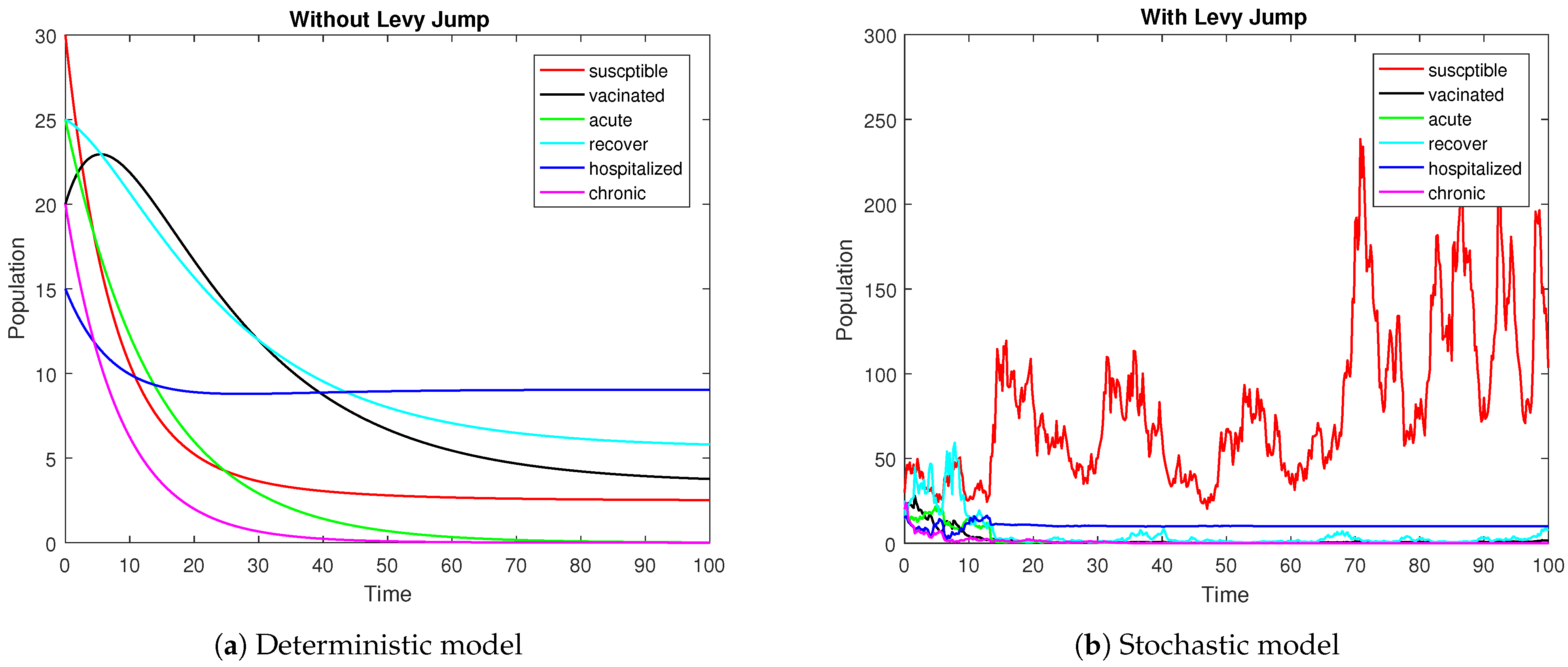
5. The HBV Extinction

In this section, we present conditions that are adequate for the extinction of the disease. Our approach begins with the introduction of two pivotal lemmas, followed by the determination of the threshold number for model (3), and then culminates in presenting the extinction of the disease.

Lemma 2. 

Consider $Z\left(t\right)$ as the solution to model (3) with any given initial value $Z\left(0\right)=Z_0$. Then, we have the following:

$$\begin{array}{cc}\hfill \underset{t\to \infty }{lim}\frac{S\left(t\right)}{t}& =0,\hfill \\ \hfill \underset{t\to \infty }{lim}\frac{I_1\left(t\right)}{t}& =0,\hfill \\ \hfill \underset{t\to \infty }{lim}\frac{I_2\left(t\right)}{t}& =0,\hfill \\ \hfill \underset{t\to \infty }{lim}\frac{H\left(t\right)}{t}& =0,\hfill \\ \hfill \underset{t\to \infty }{lim}\frac{R\left(t\right)}{t}& =0,\hfill \\ \hfill \underset{t\to \infty }{lim}\frac{V\left(t\right)}{t}& =0.\hfill \end{array}$$

(16)

Lemma 3. 

Assuming that Assumption 2 is satisfied and $Z\left(t\right)$ represents the solution to model (3) with an initial value $Z_0=Z\left(0\right)$ in the positive portion of the space $R^6$, that is, $Z_0\in R_{+}^6$, then we have the following:

$$\begin{array}{cc}\hfill & \underset{t\to \infty }{lim}\frac{{\int }_0^{t}S\left(s\right)d{W}_1\left(s\right)}{t}=\underset{t\to \infty }{lim}\frac{{\int }_0^t{I}_1\left(s\right)d{W}_2\left(s\right)}{t}=\underset{t\to \infty }{lim}\frac{{\int }_0^t{I}_2\left(s\right)d{W}_3\left(s\right)}{t}=0,\hfill \\ & \underset{t\to \infty }{lim}\frac{{\int }_0^{t}H\left(s\right)d{W}_4\left(s\right)}{t}=\underset{t\to \infty }{lim}\frac{{\int }_0^{t}R\left(s\right)d{W}_5\left(s\right)}{t}=\underset{t\to \infty }{lim}\frac{{\int }_0^{t}V\left(s\right)d{W}_6\left(s\right)}{t}=0.a.s.\hfill \\ \hfill & \mathit{Also}\hfill \\ & \underset{t\to \infty }{lim}\frac{{\int }_0^t{\int }_X{\delta }_1\left(x\right)S\left(s\right)\tilde{N}(ds,dx)}{t}=\underset{t\to \infty }{lim}\frac{{\int }_0^t{\int }_X{\delta }_2\left(x\right)I_1\left(s\right)\tilde{N}(ds,dx)}{t}=0,\hfill \\ & \underset{t\to \infty }{lim}\frac{{\int }_0^t{\int }_X{\delta }_3\left(x\right)I_2\left(s\right)\tilde{N}(ds,dx)}{t}=\underset{t\to \infty }{lim}\frac{{\int }_0^t{\int }_X{\delta }_4\left(x\right)H\left(s\right)\tilde{N}(ds,dx)}{t}=0,\hfill \\ & \underset{t\to \infty }{lim}\frac{{\int }_0^t{\int }_X{\delta }_5\left(x\right)R\left(s\right)\tilde{N}(ds,dx)}{t}=\underset{t\to \infty }{lim}\frac{{\int }_0^t{\int }_X{\delta }_6\left(x\right)V\left(s\right)\tilde{N}(ds,dx)}{t}=0.\hfill \end{array}$$

(17)

As the proofs for Lemmas 2 and 3 are very close to those of Lemma 3.1 [30] and Lemma 2.2 [31], respectively, we opt to exclude them in this particular context.

Subsequently, ensuring $Z_2\left(x\right)<1$, $\forall x\in X$, we calculate the threshold number associated with the stochastic system (3) as follows:

$$R_0=\frac{{\beta }_1+{\beta }_2+{\beta }_3+{\beta }_4}{({\alpha }_2+{\alpha }_1+{\Psi }_1+\frac{{\delta }_2^2}{t}+\chi +{\int }_X[log(1+Z_2\left(x\right))+Z_2\left(x\right)]v\left(dx\right))}.$$

(18)

The subsequent theorem explains sufficient conditions for HBV extinction using $R_0$ and the two previously stated lemmas:

Theorem 2. 

Consider that Assumption 2 holds, and $Z\left(t\right)$ is the solution of system (3) for any initial value $Z_0\in R_{+}^6$. Accordingly, for $R_0<0$, the following property holds:

$$\underset{t\to \infty }{lim}\frac{log〈I_1\left(t\right)〉}{t}<0,and\underset{t\to \infty }{lim}\frac{log〈I_2\left(t\right)〉}{t}<0,a.s.$$

(19)

As a result, $I_1\left(t\right)$ and $I_2\left(t\right)$ go to zero, guaranteeing the elimination of the disease with a high degree of probability.

Thus, we have the following:

$$\begin{array}{cc}\hfill \underset{t\to \infty }{lim}〈S\left(t\right)〉& =\frac{\Psi (\eta +\chi \Pi )}{\chi (\eta +\lambda +\chi )},\hfill \\ \hfill \underset{t\to \infty }{lim}〈I_1\left(t\right)〉& =\underset{t\to \infty }{lim}〈I_2\left(t\right)〉=0,\hfill \\ \hfill \underset{t\to \infty }{lim}〈H\left(t\right)〉& =0=\underset{t\to \infty }{lim}〈R\left(t\right)〉,\hfill \\ \hfill \underset{t\to \infty }{lim}〈V\left(t\right)〉& =\frac{\chi \Psi (1-\Pi )(\eta +\chi +\lambda )+\gamma \Psi (\eta +\chi \Pi )}{\chi (\eta +\chi +\lambda )(\chi +\eta )}.\hfill \end{array}$$

(20)

Proof. 

For the detailed proof, see Section 9. □

6. Persistence

This section discusses the long-term survival of HBV within the community. To be more precise, we will explore the conditions on the parameters that ensure the persistence of the disease, which is necessary before implementing a successful control program. We will begin by reviewing the definition of average persistence as outlined in [32].

Definition 1 

([33,34]). As long as the following conditions hold, model (3) will persist or remain durable, as follows:

$$\underset{t\to \infty }{lim}inf\frac{1}{t}{\int }_0^t{I}_1\left(r\right)>0a.s.$$

(21)

To examine HBV persistence, we need to consider the following lemmas, which are stated in [16,17].

Lemma 4 

(Strong Law [33,35]). For a continuous and real-valued local martingale function $M={\left\{M\right\}}_{0\le t}\exists$ that vanishes as $t\to 0$, we have the following:

$$\begin{array}{cc}\hfill \underset{t\to \infty }{lim}〈M,M〉& =\infty ,a.s.,⟹\underset{t\to \infty }{lim}\frac{M_t}{{〈M,M〉}_t}=0,a.s.\hfill \\ & \underset{t\to \infty }{lim}sup\frac{{〈M,M〉}_t}{t}<0,a.s.,⟹\underset{t\to \infty }{lim}\frac{M_t}{t}=0,a.s.\hfill \end{array}$$

(22)

Lemma 5. 

Suppose $h\in C\left(\right[0,\infty )\times \Omega ,(0,\infty \left)\right)$ and $\mathfrak{H}\in C([0,\infty )\times \Omega ,R)\ni {lim}_{t\to \infty }\frac{\mathfrak{H}\left(\mathfrak{t}\right)}{t}=0$. a.s. If $\forall t\ge 0$

$$logh\left(t\right)\ge -\lambda {\int }_0^{t}h\left(s\right)ds+{\lambda }_{0}t+\mathfrak{H}\left(\mathfrak{t}\right)a.s.$$

(23)

Then

$$\underset{t\to \infty }{lim}〈h\left(t\right)〉\ge \frac{{\lambda }_0}{\lambda }a.s.$$

(24)

Here, λ and ${\lambda }_0$ are, respectively, positive and non-negative real numbers.

Here, we will elucidate the criteria for the mean persistence of HBV subject to system (3), with the subsequent discussion guided by the following key parameters.

The threshold parameter associated with the stochastic model is denoted by $R_0^s$, defined as follows:

$$R_0^s=\frac{{\beta }_2\Psi \Pi }{(\gamma +\chi +\frac{{\delta }_1^2}{2}+{\int }_X[Z_1\left(x\right)-log(1+Z\left(x\right))]vdx)({\alpha }_1+{\alpha }_2+{\Psi }_1+\chi +\frac{{\delta }_2^2}{2}+{\int }_X[Z_1\left(x\right)-log(1+Z_2\left(x\right))]vdx)}.$$

(25)

Theorem 3. 

If $R_0^s>1$, then for the initial data, $(S_0,I_{10},I_{20},H_0,R_0,V_0)\in R_{+}^6$, the acutely infected population $I_1\left(t\right)$ has the following property:

$$\underset{t\to \infty }{lim}〈I_1\left(t\right)〉\ge \frac{2\Psi \Pi (\sqrt{R_0^s}-1)}{C_1{\beta }_1}a.s.$$

(26)

and similar for $lim{inf}_{t\to \infty }〈I_2\left(t\right)〉\ge 0,$ where $C_1=\frac{\Psi \Pi }{(\gamma +\chi +\frac{{\delta }_1^2}{2}+{\int }_X[Z_1\left(x\right)-log(1+Z\left(x\right))]vdx)}$. These properties of the infected compartments ensure the existence of the infection at all times in the population.

Proof. 

For a detailed proof, visit Section 10. □

Remarks

When investigating stochastic epidemic models, the terms ‘extinction’ and ‘persistence’ are frequently used. Persistence in this context refers to the continual presence of the infection within the population at any time t. If a stochastic model exhibits persistence, the stochastic curves will always be non-zero, and over the long term, these curves will oscillate around the endemic fixed point of the associated deterministic model. The extinction property indicates that the disease will be definitively eliminated from the population in the long term. Both properties are crucial to analyze in any epidemic study. Persistence alerts researchers to the need for implementing control programs, while extinction suggests to stakeholders that they can reduce their efforts, as the disease will disappear within a specified time period.

7. Numerical Model Analysis

There are two primary objectives of this section. The first aim of this part is the development of a scheme for the proposed model (3) while utilizing a standard numerical method for stochastic DEs. This will help us implement the model in MATLAB as well as decrease the computational cost. Secondly, this section offers several examples to demonstrate the model’s behaviors and validate the various theoretical results obtained so far. By achieving these aims, we can better understand the long-term behavior of the model, predict parameters that contribute to the extinction of the disease, identify parameters that are responsible for the persistence of the infection, and most importantly, delineate the strategies that are beneficial for obtaining the numerical solutions of any stochastic system.

7.1. Milstein Scheme for the Model with Jumps

In order to develop a scheme to numerically solve system (3), we will use the standard numerical method elaborated on in [36]. Various features and characteristics of the method, like stability, convergence, implementation, etc., have been rigorously investigated by many researchers; for a detailed analysis, see [37,38,39]. For a successful implementation of the method, we take $n=0,1,2\dots ,N^{*}$, where $N^{*}\in N$, $x^{*}\in X$. For discretization of the time interval $[0,T]$, we assume the uniform step-size $\Delta t=\frac{T}{N^{*}}$. Additionally, for $i\in 1,2,N_i^n=S_i^n+I_{1i}^n+I_{2i}^n+H_i^n+R_i^n+V_i^n+$, and $\Delta W_{i,n}\triangleq W\left(t_{n+1}\right)-W\left(t_n\right)=\sqrt{\Delta t}{\xi }_{i,n},$ where ${\xi }_{i,n}$ denotes the Gaussian noises with distributions $N(0,1)$. In addition, $\Delta L_n$, defined as $L\left(t_{n+1}\right)-L\left(t_n\right)$, follows a Poisson distribution with intensity v when considering $X=(0,+\infty )$ with $v\left(X\right)=1$. As a result, the numerical Milstein approach associated with model (3) assumes the following form:

$$\begin{array}{cc}\hfill S^{n+1}=& S^n+\left[\Psi \Pi -\frac{{\beta }_1{S}^n{I}_1^n}{N_1^n}-\frac{{\beta }_2{S}^n{I}_2^n}{N_1^n}+\eta V^n-(\gamma +\chi )S^n\right]\Delta t+{\delta }_1{S}^n{B}_{n,1}+\frac{{\delta }_1^2}{2}{S}^n(\Delta B_{1,n}^2-\Delta t)-Z_1\left(x^{*}\right)S^n\Delta L_n,\hfill \\ \hfill I_1^{n+1}=& I_1^n+\left[\frac{{\beta }_1{S}^n{I}_1^n}{N^n}+\frac{{\beta }_2{S}^n{I}_2^n}{N^n}+\frac{{\beta }_3{V}^n{I}_1^n}{N^n}+\frac{{\beta }_4{V}^n{I}_2}{N^n}-({\alpha }_1+{\alpha }_2+{\Psi }_1+\chi )I_1^n\right]\Delta t\hfill \\ & +{\delta }_2{I}_1^n{B}_{n,2}+\frac{{\delta }_2^2}{2}{I}_1^n(\Delta B_{2,n}^2-\Delta t)-Z_2\left(x^{*}\right)I_1^n\Delta L_n,\hfill \\ \hfill I_2^{n+1}=& I_2^n+\left[{\alpha }_1{I}_1^n-({\gamma }_1+{\Psi }_2+{\gamma }_2+\chi )I_2^n\right]\Delta t+{\delta }_3{I}_2^n{B}_{n,3}+\frac{{\delta }_3^2}{2}{I}_2^n(\Delta B_{3,n}^2-\Delta t)-Z_3\left(x^{*}\right)I_2^n\Delta L_n,\hfill \\ \hfill H^{n+1}=& H^n+[{\Psi }_1{I}_1^n+{\Psi }_2{I}_2^n-({\Psi }_3+{\Psi }_4+\chi )H^n]\Delta t+{\delta }_4{H}^n{B}_{n,4}+\frac{{\delta }_4^2}{2}{H}_2^n(\Delta B_{4,n}^2-\Delta t)-Z_4\left(x^{*}\right)H^n\Delta L_n,\hfill \\ \hfill R^{n+1}=& R^n+\left[{\gamma }_1{I}_2^n+{\alpha }_2{I}_1^n+{\Psi }_3{H}^n-\chi R^n\right]\Delta t+{\delta }_5{R}^n{B}_{n,5}+\frac{{\delta }_5^2}{2}{R}_2^n(\Delta B_{5,n}^2-\Delta t)-Z_5\left(x^{*}\right)H^n\Delta L_n,\hfill \\ \hfill V^{n+1}=& V^n+\left[\Psi (1-\Pi )+\gamma S^n-\frac{{\beta }_3{V}^n{I}_1^n}{N^n}-\frac{{\beta }_4{V}^n{I}_2^n}{N}-(\eta +\chi )V^n\right]\Delta t+{\delta }_6{V}^n{B}_{n,6}\hfill \\ & +\frac{{\delta }_6^2}{2}{V}_2^n(\Delta B_{6,n}^2-\Delta t)-Z_6\left(x^{*}\right)V^n\Delta L_n.\hfill \end{array}$$

Apart from the above-mentioned scheme, one can utilize an alternative numerical method like the positive preserving truncated Euler–Maruyama (PPTEM) method [39] to obtain numerical solutions to the model. PPTEM techniques have also been used by several authors and certain complex problems have been tackled therein; see [40] and the references cited therein. In this case, the choice of this approach is prompted by its simplicity and effectiveness in managing Lévy jumps.

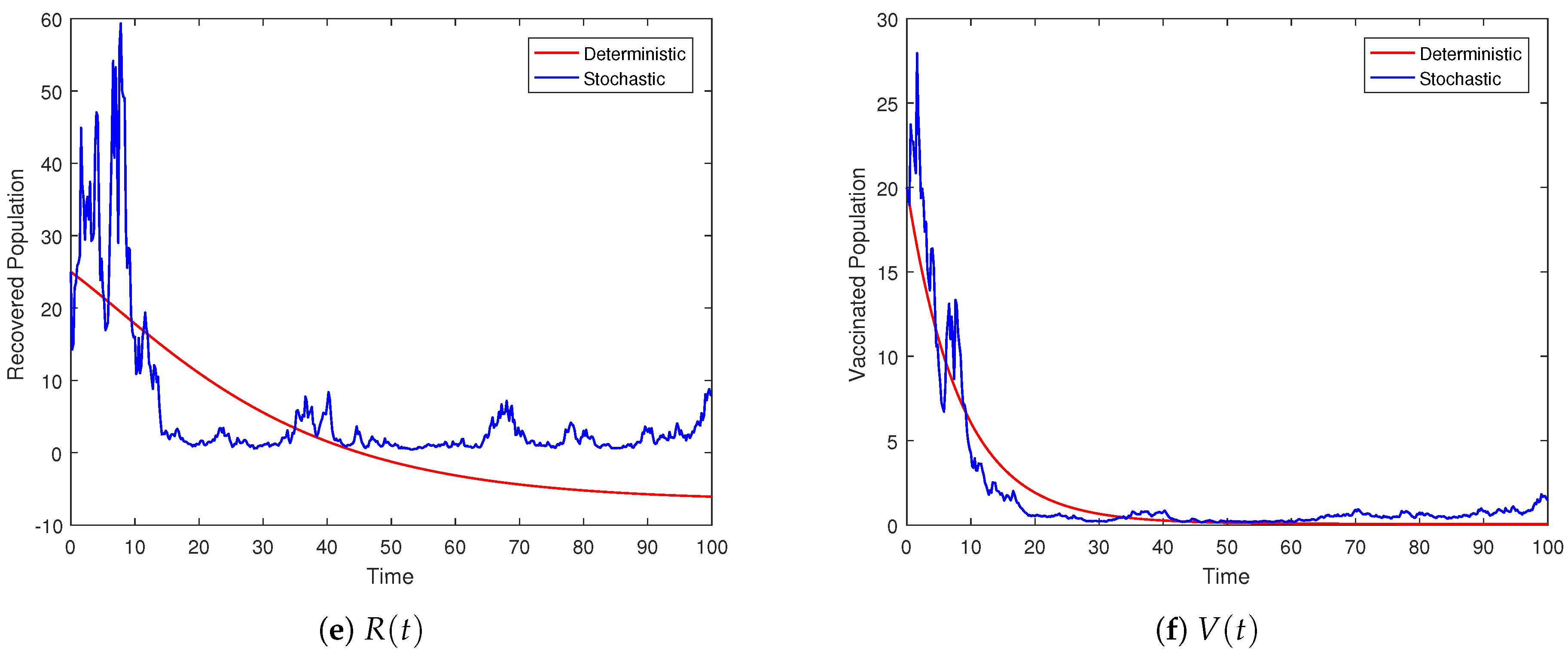
7.2. Extinction-Based Simulation

In this subsection, we will employ the developed scheme and obtain the approximate solutions of both systems. The dynamics of the stochastic model may be better understood if we simulate both the deterministic and stochastic models and the behavior of the system may be understood from the graphical illustrations. Figure 1 is the graphical representation of both stochastic and deterministic models of (3). The desired time interval is $[0,100]$, whereas, the initial approximations are $(S_0,I_{10},I_{20},H_0,R_0,V_0)=(30,25,20,15,25,20)$, and $\Delta t=0.1$. First, we will numerically verify the conclusion of Theorem 2 whenever the hypothesis of the theorem holds true. To prove this, we consider values of the parameters and intensities of the noises as {$\Psi =0.3;$ $\Pi =1,$ ${\beta }_1=0.002,$ ${\beta }_2=0.005,$ ${\beta }_3=0.0019,$ ${\beta }_4=0.002,$ $\eta =0.07,$ $\gamma =0.04,$ ${\gamma }_1=0.0025,$ ${\gamma }_2=0.01,$ $\chi =0.05,$ ${\alpha }_1=0.0025,$ ${\alpha }_2=0.003,$ ${\psi }_1=0.017,$ ${\psi }_2=0.0035,$ ${\psi }_3=0.031,$ ${\psi }_4=0.022,$ ${\delta }_1=0.05,$ ${\delta }_2=0.5,$ ${\delta }_3=0.06,$ ${\delta }_4=0.6,$ ${\delta }_5=0.63,$ ${\delta }_6=0.005,$ $Z_1=0.1,$ $Z_2=0.2,$ $Z_3=0.02,$ $Z_4=0.01,$ $Z_5=0.03,$ $Z_6=0.03$}.

Figure 2 depicts the trajectories of the compartments $(S,I_1,I_2,H,R,V)$ for different scenarios. We can observe that the stochastic curves fluctuate around the infection-free state of the associated deterministic system. The intensity of the noises is directly related to the amplitude of the oscillations. Smaller values of ${\delta }_i$ lead to oscillations with smaller amplitudes, and negligibly small values result in almost deterministic curves. For the threshold parameter $R_0^D<1$, associated with the deterministic model, the DFE is globally stable. Under the same condition on the parameters, the proposed model (3) with Lévy jumps approaches the infection-free state as time evolves. Theorem 2 ensures disease elimination whenever the hypothesis holds true, as reflected in Figure 2 via the simulation model (3). The graphical illustrations show that Theorem 2 is guaranteed whenever the threshold number $R_0<1$.

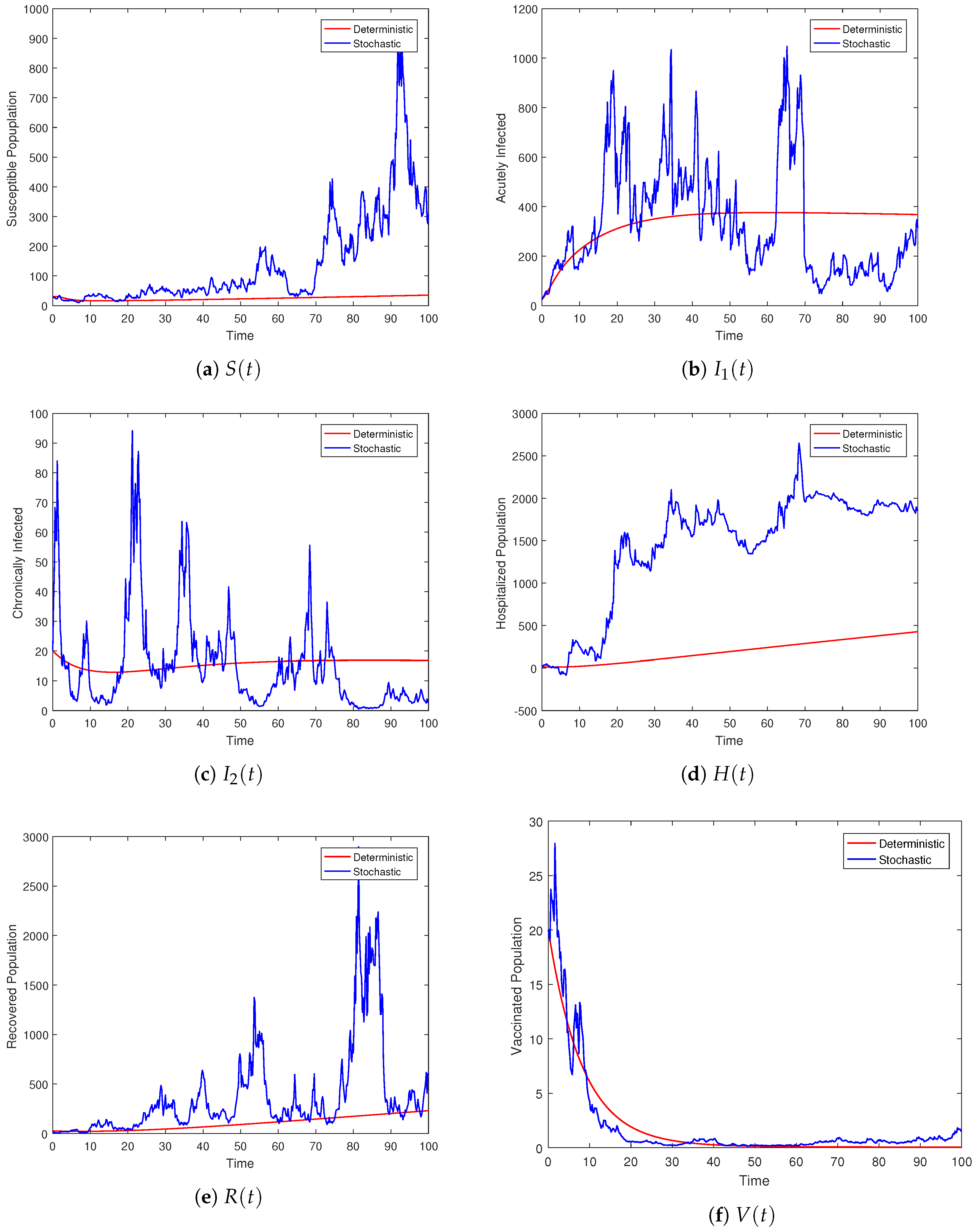
7.3. Simulation Based on Persistence of HBV

In this subsection, we attempt to numerically verify the persistence of HBV in the population. Theoretically, Theorem 3 explains the mean existence of the infection within the population. The theorem states that whenever the hypothesis is true, the conclusion follows. Figure 3 represents model (3) persistency for both deterministic and stochastic form. To prove the persistence of the stochastic model (3), we will consider values of the parameters as {$\Psi =0.3;$ $\Pi =1,$ $\beta 1=1.2;$ $\beta 2=1.5;$ $\beta 3=1.19;$ $\beta 4=0.9;$ $\eta =0.07;$ $\gamma =0.001;$ $\gamma 2=0.01;$ $\chi =0.05;$ $\alpha 1=0.0025;$ $\alpha 2=0.003;$ $\Psi 1=0.017;$ $\gamma 1=0.0025;$ $\Psi 2=0.0035;$ $\Psi 3=0.031;$ $\Psi 4=0.022;$ ${\delta }_1=0.06,$ ${\delta }_2=0.6,$ ${\delta }_3=0.07,$ ${\delta }_4=0.7,$ ${\delta }_5=0.64,$ ${\delta }_6=0.006,$ $Z_1=0.2,$ $Z_2=0.3,$ $Z_3=0.03,$ $Z_4=0.02,$ $Z_5=0.04,$ $Z_6=0.04$}. These values of the parameters satisfy the assumption of the theorem and, hence, by closely observing the graphical results in Figure 4, one can follow the conclusion of the theorem. The figure shows that all the solution curves $(S\left(t\right),I_1\left(t\right),I_2\left(t\right),H\left(t\right),R\left(t\right),V\left(t\right))$ persist in the mean, indicating that the disease will not vanish over an infinite time span. In this scenario, the deterministic curves will approach the endemic fixed point, while the stochastic curves will oscillate around this endemic state of the model. Here, the amplitude of the oscillations depends on the intensity of the noises.

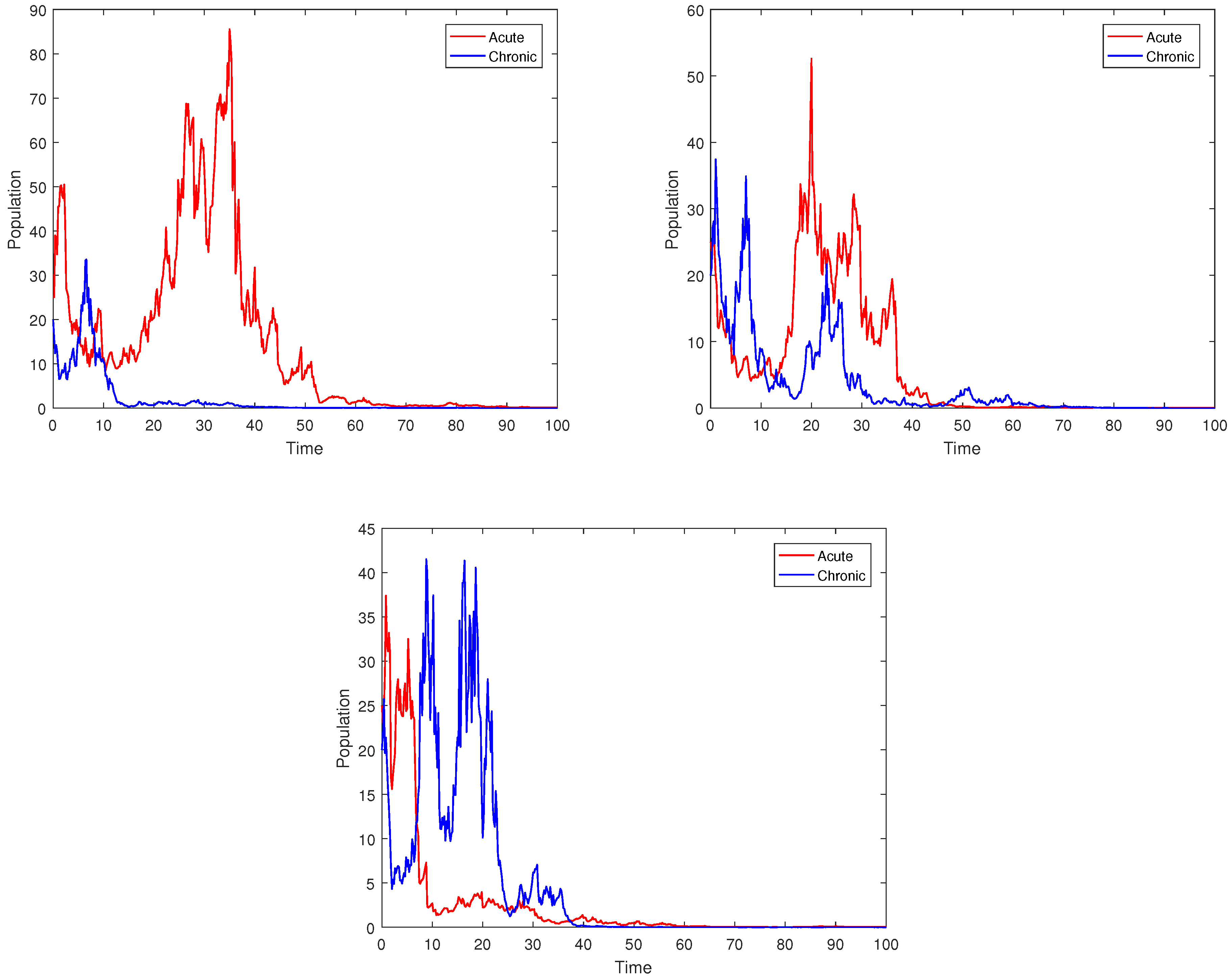
7.4. The Impact of Noise on the Stochastic System (3)

To check the impact of the noise on the dynamics of the stochastic system (3), we set the parameter values as $\{\Psi =0.3;$ $\Pi =1,$ ${\beta }_1=0.002,$ ${\beta }_2=0.005,$ ${\beta }_3=0.0019,$ ${\beta }_4=0.002,$ $\eta =0.07,$ $\gamma =0.001,$ ${\gamma }_1=0.0025,$ ${\gamma }_2=0.01,$ $\chi =0.05,$ ${\alpha }_1=0.0025,$ ${\alpha }_2=0.003,$ ${\psi }_1=0.017,$ ${\psi }_2=0.0035,$ ${\psi }_3=0.031,$ ${\psi }_4=0.022\}$ and choose $\{{\delta }_1,{\delta }_2,{\delta }_3,{\delta }_4,{\delta }_5,{\delta }_6\}=\{(0.01,0.6,0.001,0.006,0.2,0.01),(0.05,0.2,0.005,0.002,0.1,0.001),(0.006,0.7,0.007,0.006,0.25,0.1)\}$, {$Z_1,Z_2,Z_3,Z_4,Z_5,Z_6\}=\left\{\right(0.1,0.5,0.05,0.01,0.6,0.08),(0.1,0.2,0.002,0.01,0.3,0.9),(0.2,0.3,0.002,0.003,0.5,0.6\left)\right\}$. Figure 5 depicts the associated partial solutions of model (3) in terms of the sizes of the acute and chronic infections, together with the average infected relative cure. According to the simulation findings, small noises in the environment have a substantial effect on the populations of $I_1\left(t\right)$ and $I_2\left(t\right)$, as well as the average relative infections.

7.5. Vaccination Impact on the Stochastic System (3)

To check the vaccination impact on the dynamics of the stochastic system (3), we set parameter values as {$\Psi =0.3;$ $\Pi =1,$ $\beta 1=1.2;$ $\beta 2=1.5;$ $\beta 3=1.19;$ $\beta 4=0.9;$ $\eta =0.07;$ $\gamma 2=0.01;$ $\chi =0.05;$ $\alpha 1=0.0025;$ $\alpha 2=0.003;$ $\Psi 1=0.017;$ $\gamma 1=0.0025;$ $\Psi 2=0.0035;$ $\Psi 3=0.031;$ $\Psi 4=0.022;$ ${\delta }_1=0.06,$ ${\delta }_2=0.6,$ ${\delta }_3=0.07,$ ${\delta }_4=0.7,$ ${\delta }_5=0.64,$ ${\delta }_6=0.006,$ $Z_1=0.2,$ $Z_2=0.3,$ $Z_3=0.03,$ $Z_4=0.02,$ $Z_5=0.04,$ $Z_6=0.04$}. Moreover, $\gamma =\{0.02,0.04,0.08\}$ Figure 6 depicts the associated partial solutions of the model (3) in terms of the sizes of the acute and chronic infections, together with the average infected relative cure. According to the simulation findings, lowering the rate of vaccination will help the disease to spread faster in the population.

7.6. The Impact of $\beta$ on Stochastic System (3)

To show the relative impact of the parameter $\beta$ on the dynamics of the stochastic model, we take values of the parameters, such as ${\beta }_1=(0.002,0.004,0.008)$, ${\beta }_2=(0.005,0.010,0.020)$, ${\beta }_3=(0.0019,0.0038,0.0076)$ and ${\beta }_4=(0.002,0.004,0.008)$, along with other parameters, such as {$\Psi =0.3;$ $\Pi =1,$ $\eta =0.07,$ $\gamma =0.001,$ ${\gamma }_1=0.0025,$ ${\gamma }_2=0.01,$ $\chi =0.05,$ ${\alpha }_1=0.0025,$ ${\alpha }_2=0.003,$ ${\psi }_1=0.017,$ ${\psi }_2=0.0035,$ ${\psi }_3=0.031,$ ${\psi }_4=0.022,$ ${\delta }_1=0.05,$ ${\delta }_2=0.5,$ ${\delta }_3=0.06,$ ${\delta }_4=0.6,$ ${\delta }_5=0.63,$ ${\delta }_6=0.005,$ $Z_1=0.1,$ $Z_2=0.2,$ $Z_3=0.02,$ $Z_4=0.01,$ $Z_5=0.03,$ $Z_6=0.03$}. Figure 7 shows the dynamics of the acute and chronic populations and the average relative infections using the suggested stochastic model. The figure suggests that lowering the value of $\beta$ accelerates disease extinction in the respective populations. This means that to accomplish disease extinction, the values of $\beta$ should be reduced. Furthermore, our simulations demonstrate the significance of using nonlinear stochastic disturbances in order to better understand HBV dynamics.

8. Conclusions

In this manuscript, we investigated a stochastic $S{I}_1{I}_{2}HRV$ epidemic model that governs the dynamic behavior of the HBV infection subject to the Brownian motion, Lévy jumps, and the nonlinear rate of incidence. The white noises are included to account for small fluctuations, and to capture sudden changes, we incorporated Lévy noises into the model. After formulating the model, we studied the existence of a global positive solution. The behavior of the stochastic model is investigated around the infection-free and endemic states of the underlying ODE system. We derived sufficient conditions for both the elimination and persistence of HBV. The oscillations of the stochastic curves are subject to the intensities of white noises and Lévy jumps. It was noticed that smaller values of the intensities and jumps lead to smaller oscillations of the curves in the vicinity of the fixed points of the ODE model. We simulated the model by using the standard numerical method; moreover, multiple scenarios were discussed. The majority of theoretical findings in this study are validated through simulations, and the relative impacts of certain parameters on the disease dynamics were thoroughly elaborated. Considering the importance of this study and identifying certain gaps, the authors intend to explore the effect of different noises on the dynamics of other infectious diseases utilizing $SVIS$ and $SEIR$ models.

The main outcomes of this study are the stochastic epidemic model, the global positive solution, the behavior around infection states, the infection-free state, the endemic state, conditions for elimination and existence, oscillation and noise, simulation, validation, and future directions for $SVIS$ and $SEIR$ models. This study contributes to our understanding of HBV infection dynamics under stochastic effects and provides valuable insights into disease control and management.

The limitation of this paper is that we did not discuss the population class who recover and then become susceptible again due to their weak immune systems. Addressing this issue will be the focus of our future work, where we will design a model for that class.

9. Proof of Theorem 2

Proof. 

The following calculation is obtained when the model (3) is directly integrated.

$$\begin{array}{cc}\hfill \frac{S\left(t\right)-S\left(0\right)}{t}=& \Psi \Pi -\frac{{\beta }_1〈S\left(t\right)I_1\left(t\right)〉}{〈N〉}-\frac{{\beta }_2〈S\left(t\right)I_2\left(t\right)〉}{〈N〉}+\eta 〈V\left(t\right)〉-(\gamma +\chi )〈S\left(t\right)〉\hfill \\ & +\frac{{\delta }_1}{t}{\int }_0^{t}S\left(r\right)B_1\left(r\right)+\frac{1}{t}{\int }_0^t\left[{\int }_X{Z}_1\left(x\right)S\left(t^{-}\right)\tilde{N}(dt,dx)\right]dr,\hfill \\ \hfill \frac{I_1\left(t\right)-I_1\left(0\right)}{t}=& \frac{{\beta }_1〈S\left(t\right)I_1\left(t\right)〉}{〈N〉}+\frac{{\beta }_2〈S\left(t\right)I_2\left(t\right)〉}{〈N〉}+\frac{{\beta }_3〈V\left(t\right)I_1\left(t\right)〉}{〈N〉}+\frac{{\beta }_4〈V\left(t\right)I_2\left(t\right)〉}{〈N〉}\hfill \\ \hfill & -({\alpha }_1+{\alpha }_2+{\Psi }_1+\chi )〈I_1\left(t\right)〉+\frac{{\delta }_2}{t}{\int }_0^t{I}_1\left(r\right)B_2\left(r\right)+\frac{1}{t}{\int }_0^t\left[{\int }_X{Z}_2\left(x\right)I_1\left(t^{-}\right)\tilde{N}(dt,dx)\right]dr,\hfill \\ \hfill \frac{I_2\left(t\right)-I_2\left(0\right)}{t}=& {\alpha }_1〈I_1\left(t\right)〉-({\gamma }_1+{\Psi }_2+{\gamma }_2+\chi )〈I_2\left(t\right)〉\hfill \\ \hfill & +\frac{{\delta }_3}{t}{\int }_0^t{I}_2\left(r\right)B_3\left(r\right)+\frac{1}{t}{\int }_0^t\left[{\int }_X{Z}_3\left(x\right)I-2\left(t^{-}\right)\tilde{N}(dt,dx)\right]dr,\hfill \\ \hfill \frac{H\left(t\right)-H\left(0\right)}{t}=& {\Psi }_1〈I_1\left(t\right)〉+{\Psi }_2〈I_2\left(t\right)〉-({\Psi }_3+{\Psi }_4+\chi )〈H\left(t\right)〉\hfill \\ \hfill & +\frac{{\delta }_4}{t}{\int }_0^{t}H\left(r\right)B_4\left(r\right)+\frac{1}{t}{\int }_0^t\left[{\int }_X{Z}_4\left(x\right)H\left(t^{-}\right)\tilde{N}(dt,dx)\right]dr,\hfill \\ \hfill \frac{R\left(t\right)-R\left(0\right)}{t}=& {\gamma }_1〈I_2\left(t\right)〉+{\alpha }_2〈I_1\left(t\right)〉+{\Psi }_3〈H\left(t\right)〉-\chi 〈R\left(t\right)〉+\hfill \\ \hfill & \frac{{\delta }_1}{t}{\int }_0^{t}R\left(r\right)B_5\left(r\right)+\frac{1}{t}{\int }_0^t\left[{\int }_X{Z}_5\left(x\right)R\left(t^{-}\right)\tilde{N}(dt,dx)\right]dr,\hfill \\ \hfill \frac{V\left(t\right)-V\left(0\right)}{t}=& \Psi (1-\Pi )+\gamma 〈S\left(t\right)〉-\frac{{\beta }_3〈V\left(t\right)I_1\left(t\right)〉}{〈N〉}-\frac{{\beta }_4〈V\left(t\right)I_2\left(t\right)〉}{〈N〉}-(\eta +\chi )〈V\left(t\right)〉\hfill \\ & +\frac{{\delta }_6}{t}{\int }_0^{t}V\left(r\right)B_6\left(r\right)+\frac{1}{t}{\int }_0^t\left[{\int }_X{Z}_6\left(x\right)V\left(t^{-}\right)\tilde{N}(dt,dx)\right]dr.\hfill \end{array}$$

(27)

By applying Itô’s formula to the function $G=log{I}_1\left(t\right)$

$$dlog{I}_1\left(t\right)=LG\left(t\right)+{\delta }_{2}d{B}_2\left(t\right)+{\int }_X[log(1+Z_2\left(x\right))]\tilde{N}(dt,dx).$$

(28)

Taking the integration of Equation (28) in the interval $[0,t]$ with division by t, we obtain the following:

$$\begin{array}{cc}\hfill \frac{log{I}_1\left(t\right)-log{I}_1\left(t\right)}{t}& =\frac{{\beta }_1〈S\left(t\right)〉}{〈N〉}+\frac{{\beta }_2〈S\left(t\right)I_2\left(t\right)〉}{〈N〉}+\frac{{\beta }_3〈V\left(t\right)〉}{〈N〉}+\frac{{\beta }_4〈V\left(t\right)I_2\left(t\right)〉}{〈N〉}-({\alpha }_1+{\alpha }_2+{\Psi }_1+\chi )\hfill \\ & -\frac{{\delta }_2^2}{t}+\frac{{\delta }_2}{t}{\int }_0^{t}d{B}_2\left(r\right)+\frac{1}{t}{\int }_X[log(1+Z_2\left(x\right)]\tilde{N}(dt,dx)-{\int }_X[Z_2\left(x\right)-log(1+Z_2\left(x\right))]vdx,\hfill \\ \hfill \le & {\beta }_1+{\beta }_2+{\beta }_3+{\beta }_4-\left({\alpha }_1+{\alpha }_2+{\Psi }_1+\chi +\frac{{\delta }_2^2}{t}+{\int }_X[Z_2\left(x\right)-log(1+Z_2\left(x\right))]vdx\right)+\frac{{\delta }_2}{t}{\int }_0^{t}d{B}_2\left(r\right)\hfill \\ & +\frac{1}{t}{\int }_X[log(1+Z_2\left(x\right)]\tilde{N}(dt,dx).\hfill \end{array}$$

(29)

Let $M\left(t\right)=\frac{{\delta }_2}{t}{\int }_0^{t}d{B}_2\left(r\right)+\frac{1}{t}{\int }_X[log(1+Z_2\left(x\right)]\tilde{N}(dt,dx)$, which is known as a locally continuous integral if $M\left(0\right)=0$.

From Lemma 2 and with $t\to \infty$, we have the following:

$$\underset{t\to \infty }{lim}sup\frac{M\left(t\right)}{t}=0.$$

(30)

If $R_0<1$ is satisfied, then Equation (29) is as follows:

$$\underset{t\to \infty }{lim}sup\frac{log{I}_1\left(t\right)}{t}\le \left[{\alpha }_1+{\alpha }_2+{\Psi }_1+\chi +\frac{{\delta }_2^2}{t}+{\int }_X[Z_2\left(x\right)-log(1+Z_2\left(x\right))]vdx\right](R_0-1)<0a.s.$$

(31)

Equation (31) implies the following:

$$\underset{t\to \infty }{lim}{I}_1\left(t\right)=0a.s.$$

(32)

In addition, we must use Equation (32) to solve the third equation of model (3). We combine this with the restriction of integration over a limited interval, that is, from 0 to t, and then divide the resulting expression by t.

$$\begin{array}{cc}\hfill \frac{I_2\left(t\right)-I_2\left(0\right)}{t}& ={\alpha }_1〈I_1\left(t\right)〉-({\gamma }_1+{\Psi }_2+{\gamma }_2+\chi )〈I_2\left(t\right)〉+\frac{{\delta }_3}{t}{\int }_0^t{I}_2\left(r\right)d{B}_3\left(r\right)+\frac{1}{t}{\int }_0^t\left[{\int }_X{Z}_3\left(x\right)I_2\left(t^{-}\right)\tilde{N}(dt,dx)\right]dr,\hfill \\ & \\ & 〈I_2\left(t\right)〉=\left(\frac{{\alpha }_2〈I_1\left(t\right)〉+\frac{I_2\left(0\right)-I_2\left(t\right)}{t}+\frac{{\delta }_3}{t}{\int }_0^t{I}_2\left(r\right)d{B}_3\left(r\right)+\frac{1}{t}{\int }_0^t\left[{\int }_X{Z}_3\left(x\right)I_2\left(t^{-}\right)\tilde{N}(dt,dx)\right]dr}{({\gamma }_1+{\Psi }_2+{\gamma }_2+\chi )}\right).\hfill \end{array}$$

(33)

This implies the following:

$$\underset{t\to \infty }{lim}〈I_2\left(t\right)〉=0,a.s.$$

(34)

Similarly, if we use Equation (32), Equation (34), and let $t\to \infty$, we can derive the remaining parts of the equation for the H and R class as follows:

$$\underset{t\to \infty }{lim}〈H\left(t\right)〉=0,and\underset{t\to \infty }{lim}〈R\left(t\right)〉=0,a.s.$$

(35)

We determine the following calculation by using Equation (27):

$$\begin{array}{cc}\hfill \frac{S\left(t\right)+V\left(t\right)-S\left(0\right)-V\left(0\right)}{t}& =\Psi \Pi +\eta 〈V\left(t\right)〉-\gamma 〈S\left(t\right)〉-\chi 〈S\left(t\right)〉+\Psi -\Psi \Pi +\gamma 〈S\left(t\right)〉-\eta 〈V\left(t\right)〉-\chi 〈V\left(t\right)〉\hfill \\ & +\frac{{\delta }_1}{t}{\int }_0^{t}S\left(r\right)d{B}_1\left(r\right)+\frac{1}{t}{\int }_0^t\left[{\int }_X{Z}_1\left(x\right)S\left(t^{-}\right)\tilde{N}(dt,dx)\right]dr\hfill \\ & +\frac{{\delta }_6}{t}{\int }_0^{t}V\left(r\right)d{B}_6\left(r\right)+\frac{1}{t}{\int }_0^t\left[{\int }_X{Z}_6\left(x\right)V\left(t^{-}\right)\tilde{N}(dt,dx)\right]dr,\hfill \\ \hfill \frac{S\left(t\right)+V\left(t\right)-S\left(0\right)-V\left(0\right)}{t}& =\Psi -\chi 〈S\left(t\right)+V\left(t\right)〉+\frac{{\delta }_1}{t}{\int }_0^{t}S\left(r\right)d{B}_1\left(r\right)+\frac{1}{t}{\int }_0^t\left[{\int }_X{Z}_1\left(x\right)S\left(t^{-}\right)\tilde{N}(dt,dx)\right]dr\hfill \\ & +\frac{{\delta }_6}{t}{\int }_0^{t}V\left(r\right)d{B}_6\left(r\right)+\frac{1}{t}{\int }_0^t\left[{\int }_X{Z}_6\left(x\right)V\left(t^{-}\right)\tilde{N}(dt,dx)\right]dr,\hfill \\ \hfill 〈S\left(t\right)+V\left(t\right)〉& =\frac{\Psi }{\chi }-\frac{1}{\chi }[\frac{S\left(t\right)-S\left(0\right)}{t}-\frac{{\delta }_1}{t}{\int }_0^{t}S\left(r\right)d{B}_1\left(r\right)+\frac{V\left(t\right)-V\left(0\right)}{t}\hfill \\ & -\frac{{\delta }_6}{t}{\int }_0^{t}V\left(r\right)d{B}_6\left(r\right)+\frac{1}{t}{\int }_0^t\left[{\int }_X{Z}_1\left(x\right)S\left(t^{-}\right)\tilde{N}(dt,dx)\right]dr\hfill \\ & +\frac{1}{t}{\int }_0^t\left[{\int }_X{Z}_6\left(x\right)V\left(t^{-}\right)\tilde{N}(dt,dx)\right]dr].\hfill \end{array}$$

(36)

Let us say that the operator $\varphi \left(t\right)$ is defined as follows:

$$\begin{array}{cc}\hfill \varphi \left(t\right)& =-\frac{1}{\chi }[\frac{S\left(t\right)-S\left(0\right)}{t}-\frac{{\delta }_1}{t}{\int }_0^{t}S\left(r\right)d{B}_1\left(r\right)+\frac{V\left(t\right)-V\left(0\right)}{t}-\frac{{\delta }_6}{t}{\int }_0^{t}V\left(r\right)d{B}_6\left(r\right)\hfill \\ & +\frac{1}{t}{\int }_0^t\left[{\int }_X{Z}_1\left(x\right)S\left(t^{-}\right)\tilde{N}(dt,dx)\right]dr+\frac{1}{t}{\int }_0^t\left[{\int }_X{Z}_6\left(x\right)V\left(t^{-}\right)\tilde{N}(dt,dx)\right]dr].\hfill \end{array}$$

(37)

Clearly, $\varphi \left(t\right)\to 0$ is the same as $t\to \infty$. So we have the following:

$$\chi 〈S\left(t\right)+V\left(t\right)〉=\Psi .$$

(38)

Thus, we estimate it using the last equation of system (27) in the same way.

$$\begin{array}{cc}\hfill \frac{V\left(t\right)-V\left(0\right)}{t}& =\Psi (1-\Pi )+\gamma 〈S\left(t\right)〉-(\eta +\chi )〈V\left(t\right)〉+\frac{{\delta }_6}{t}{\int }_0^{t}V\left(r\right)d{B}_6\left(r\right)+\hfill \\ & \frac{1}{t}{\int }_0^t\left[{\int }_X{Z}_6\left(x\right)V\left(t^{-}\right)\tilde{N}(dt,dx)\right]dr,\hfill \\ \\ \hfill \gamma 〈S\left(t\right)〉-(\eta +\chi )〈V\left(t\right)〉& =\psi (1-\Pi )-\frac{V\left(t\right)-V\left(0\right)}{t}+\frac{{\delta }_6}{t}{\int }_0^{t}V\left(r\right)d{B}_6\left(r\right)+\hfill \\ & \frac{1}{t}{\int }_0^t\left[{\int }_X{Z}_6\left(x\right)V\left(t^{-}\right)\tilde{N}(dt,dx)\right]dr.\hfill \end{array}$$

(39)

Taking $t\to \infty$, we have the following:

$$(\eta +\chi )〈V\left(t\right)〉-\gamma 〈S\left(t\right)〉=\Psi (1-\Pi ).$$

(40)

We now easily obtain the following equations for $S\left(t\right)$ and $V\left(t\right)$:

$$\underset{t\to \infty }{lim}〈S\left(t\right)〉=\frac{\Psi (\eta +\chi \Pi )}{\chi (\eta +\lambda +\chi )},a.s.$$

(41)

and

$$\underset{t\to \infty }{lim}〈V\left(t\right)〉=\frac{\chi \Psi (1-\Pi )(\eta +\lambda +\chi )+\gamma \Psi (\eta +\chi \Pi )}{\chi (\eta +\lambda +\chi )(\eta +\chi )}a.s.$$

(42)

Thus, here, we complete our proof for Theorem 2. □

10. Proof of Theorem 3

Proof. 

Set

$$L{G}_1=C_{1}L(-lnS)+C_{2}L(-ln{I}_1),$$

(43)

$C_1$ and $C_2$ are constants that we will define later.

By applying Itô’s formula to the above Equation (43), we obtain the following results:

$$\begin{array}{cc}\hfill d{G}_1=& L{G}_1-C_1{\delta }_{1}d{B}_1\left(t\right)-C_2{\delta }_{2}d{B}_2\left(t\right)-C_1{\int }_X[Z_1\left(x\right)S-log(1+Z_1\left(x\right))]\tilde{N}(dt,dx)-\hfill \\ & C_2{\int }_X[Z_2\left(x\right)I_1-log(1+Z_2\left(x\right))]\tilde{N}(dt,dx),\hfill \end{array}$$

(44)

where

$$\begin{array}{cc}\hfill L{G}_1=& C_{1}L(-lnS)+C_{2}L(-ln{I}_1),\hfill \\ & =-C_1\frac{\Psi \Pi }{S\left(t\right)}+C_1\frac{{\beta }_1{I}_1\left(t\right)}{N}-C_1\frac{{\beta }_{2}S\left(t\right)I_2\left(t\right)}{N}-C_1\frac{\eta V\left(t\right)}{S\left(t\right)}+C_1(\gamma +\chi )+C_1\frac{{\delta }_1^2}{2}+C_1\left\{{\int }_X[Z_1\left(x\right)-log(1+Z_1\left(x\right))]vdx\right\}\hfill \\ & -C_2\frac{{\beta }_{1}S\left(t\right)}{N}-C_2\frac{{\beta }_{2}S\left(t\right)I_2\left(t\right)}{N}-C_2\frac{{\beta }_{3}V\left(t\right)}{N}-C_2\frac{{\beta }_{4}V\left(t\right)I_2\left(t\right)}{N}+C_2({\alpha }_1+{\alpha }_2+{\Psi }_1+\chi )+C_2\frac{{\delta }_2^2}{2}\hfill \\ & +C_2\left\{{\int }_X[Z_2\left(x\right)-log(1+Z_2\left(x\right))]vdx\right\},\hfill \\ \hfill \le & -C_1\frac{\Psi \Pi }{S\left(t\right)}+C_1{\beta }_1+C_1({\gamma }_1+\chi )+C_1\frac{{\delta }_1^2}{2}+C_1\left\{{\int }_X[Z_1\left(x\right)-log(1+Z_1\left(x\right))]vdx\right\}\hfill \\ & -C_2{\beta }_1-C_2{\beta }_{2}S\left(t\right)-C_2{\beta }_3+C_2({\alpha }_1+{\alpha }_2+{\Psi }_1+\chi )+C_2\frac{{\delta }_2^2}{2}+C_2\left\{{\int }_X[Z_2\left(x\right)-log(1+Z_2\left(x\right))]vdx\right\},\hfill \\ \hfill \le & -2\sqrt{C_1{C}_2\Psi \Pi {\beta }_2}+C_1\left[\gamma +\chi +\frac{{\delta }_1^2}{2}+{\int }_X[Z_1\left(x\right)-log(1+Z_1\left(x\right))]vdx\right]\hfill \\ & +C_2\left[{\alpha }_1+{\alpha }_2+{\Psi }_1+\chi +\frac{{\delta }_2^2}{2}+{\int }_X[Z_2\left(x\right)-log(1+Z_2\left(x\right))]vdx\right],\hfill \end{array}$$

(45)

let

$$\begin{array}{cc}\hfill C_1=& \frac{\Psi \Pi }{\left(\gamma +\chi +\frac{{\delta }_1^2}{2}+{\int }_X[Z_1\left(x\right)-log(1+Z_1\left(x\right))]vdx\right)},\hfill \\ \hfill C_2=& \frac{\Psi \Pi }{\left({\alpha }_1+{\alpha }_2+{\Psi }_1+\chi +\frac{{\delta }_2^2}{2}+{\int }_X[Z_2\left(x\right)-log(1+Z_2\left(x\right))]vdx\right)}.\hfill \end{array}$$

(46)

Let us suppose the following:

$$\begin{array}{cc}\hfill a=& \left(\gamma +\chi +\frac{{\delta }_1^2}{2}+{\int }_X[Z_1\left(x\right)-log(1+Z_1\left(x\right))]vdx\right),\hfill \\ \hfill b=& \left({\alpha }_1+{\alpha }_2+{\Psi }_1+\chi +\frac{{\delta }_2^2}{2}+{\int }_X[Z_2\left(x\right)-log(1+Z_2\left(x\right))vdx\right).\hfill \end{array}$$

(47)

$$\begin{array}{cc}\hfill L{G}_1\le & \sqrt{\frac{{(\Psi \Pi )}^2\Psi \Pi {\beta }_2}{ab}}+2\Psi \Pi +C_1{\beta }_1{I}_1\left(t\right),\hfill \\ \hfill =& -2\Psi \Pi \left[\sqrt{\frac{{\beta }_2\Psi \Pi }{ab}}-1\right]+C_1{\beta }_1{I}_1\left(t\right),\hfill \\ \hfill =& -2\Psi \Pi \left[\sqrt{R_0^s}-1\right]+C_1{\beta }_1{I}_1\left(t\right).\hfill \end{array}$$

(48)

We put Equation (48) into Equation (43) after integrating both sides of model (3):

$$\begin{array}{cc}\hfill \frac{G_1(S\left(t\right),I_1\left(t\right))-G_1(S\left(0\right),I_1\left(0\right))}{t}\le & -2\Psi \Pi \left(\sqrt{R_0^s}-1\right)+C_1{\beta }_1{I}_1\left(t\right)-\frac{C_1{\delta }_1^2{B}_1\left(t\right)}{t}-\frac{C_2{\delta }_2^2{B}_2\left(t\right)}{t}\hfill \\ & -\frac{C_1{\int }_X\left[Z_1\left(x\right)S-log(1+Z_1\left(x\right))\right]\tilde{N}(dt,dx)}{t}\hfill \\ & -\frac{C_2{\int }_X\left[Z_2\left(x\right)I_1-log(1+Z_2\left(x\right))\right]\tilde{N}(dt,dx)}{t},\hfill \\ & \le -2\Psi \Pi \left(\sqrt{R_0^s}-1\right)+C_1{\beta }_1{I}_1\left(t\right)+\Theta \left(t\right).\hfill \end{array}$$

(49)

where

$$\begin{array}{cc}\hfill \Theta & =-\frac{C_1{\delta }_1^2{B}_1\left(t\right)}{t}-\frac{C_2{\delta }_2^2{B}_2\left(t\right)}{t}-\frac{C_1{\int }_X\left[Z_1\left(x\right)S-log(1+Z_1\left(x\right))\right]\tilde{N}(dt,dx)}{t}\hfill \\ \hfill & -\frac{C_2{\int }_X\left[Z_2\left(x\right)I_1-log(1+Z_2\left(x\right))\right]\tilde{N}(dt,dx)}{t}\hfill \end{array}$$

From the strong law, as stated in Lemma 4, we have the following:

$$\begin{array}{c}\hfill \underset{t\to \infty }{lim}\Theta \left(t\right)=0.\end{array}$$

(50)

From Equation (48), we have the following:

$$\begin{array}{c}\hfill 〈I_1\left(t\right)〉\ge \frac{2\Psi \Pi \left(\sqrt{R_0^s}-1\right)}{C_1{\beta }_1}-\frac{1}{C_1{\beta }_1}\Theta \left(t\right)+\frac{1}{C_1{\beta }_1}\left(\frac{G_1(S\left(t\right),I_1\left(t\right))-G_1(S\left(0\right),I_1\left(0\right))}{t}\right)\end{array}$$

(51)

According to Lemma 5 and Equation (50), the limit superior of Equation (9) yields the following:

$$\begin{array}{c}\hfill \underset{t\to \infty }{lim}inf〈I_1\left(t\right)〉\ge \frac{2\Pi \Psi \left(\sqrt{R_0^s}-1\right)}{C_1{\beta }_1}a.s.\end{array}$$

(52)

Similarly also for $lim{inf}_{t\to \infty }〈I_2\left(t\right)〉\ge 0.$

Hence, here, we complete our proof for Theorem 3. □

References

1. Din, A.; Li, Y.; Khan, T.; Zaman, G. Mathematical analysis of spread and control of the novel corona virus (COVID-19) in China. Chaos Solitons Fractals 2020, 141, 110286. [Google Scholar] [CrossRef] [PubMed]
2. Guo, B.; Khan, A.; Din, A. Numerical simulation of nonlinear stochastic analysis for measles transmission: A case study of a measles epidemic in Pakistan. Fractal Fract. 2023, 7, 130. [Google Scholar] [CrossRef]
3. Li, X.Z.; Wang, J.; Ghosh, M. Stability and bifurcation of an SIVS epidemic model with treatment and age of vaccination. Appl. Math Model 2010, 34, 437–450. [Google Scholar] [CrossRef]
4. Poland, G.; Jacobson, R. Prevention of hepatitis B with the hepatitis B vaccine. N. Engl. J. Med. 2001, 351, 2832–2838. [Google Scholar] [CrossRef] [PubMed]
5. McAleer, W.J.; Buynak, E.B.; Maigeter, R.Z.; Wampler, D.E.; Miller, W.; Hilleman, R. Human hepatitis B vaccine from recombinant yeast. Nature 1984, 307, 178–180. [Google Scholar] [CrossRef] [PubMed]
6. La Cognata, A.; Valenti, D.; Dubkov, A.A.; Spagnolo, B. Dynamics of two competing species in the presence of Lévy noise sources. Phys. Rev. E 2010, 82, 011121. [Google Scholar] [CrossRef] [PubMed]
7. Lisowski, B.; Valenti, D.; Spagnolo, B.; Bier, M.; Gudowska-Nowak, E. Stepping molecular motor amid Lévy white noise. Phys. Rev. E 2015, 91, 042713. [Google Scholar] [CrossRef]
8. Denaro, G.; Valenti, D.; La Cognata, A.; Spagnolo, B.; Bonanno, A.; Basilone, G.; Mazzola, S.; Zgozi, S.W.; Aronica, S.; Brunet, C. Spatio-temporal behaviour of the deep chlorophyll maximum in mediterranean sea: Development of a stochastic model for picophytoplankton dynamics. Ecol. Complex 2013, 13, 21–34. [Google Scholar] [CrossRef]
9. Giuffrida, A.; Valenti, D.; Ziino, G.; Spagnolo, B.; Panebianco, A. A stochastic interspecific competition model to predict the behaviour of listeria monocytogenes in the fermentation process of a traditional siciliansalami. Eur. Food Res. Technol. 2009, 228, 767–775. [Google Scholar] [CrossRef]
10. Carollo, A.; Spagnolo, B.; Valenti, D. Uhlmann curvature in dissipative phase transitions. Sci. Rep. 2018, 8, 9852. [Google Scholar] [CrossRef]
11. Spagnolo, B.; Cirone, M.; La Barbera, A.; de Pasquale, F. Noise-induced effects in population dynamics. J. Phys. 2002, 14, 2247. [Google Scholar] [CrossRef]
12. Din, A.; Li, Y.; Yusuf, A. Delayed hepatitis B epidemic model with stochastic analysis. Chaos Solitons Fractals 2021, 146, 110839. [Google Scholar] [CrossRef]
13. Meena, M.; Purohit, M.; Purohit, S.D.; Nisar, K.S. A nove linvestigation of the hepatitis B virus using a fractional operator with anon-local kernel. Partial Differ. Equ. Appl. Math. 2023, 8, 100577. [Google Scholar] [CrossRef]
14. Bhatter, S.; Jangid, K.; Purohit, S.D. A study of the Hepatitis B viruses infection using hilfer fractional derivative. Proc. Inst. Math. Mech. Natl. Acad. Sci. Azerbaijan 2022, 48, 100–117. [Google Scholar] [CrossRef]
15. Cui, T.; Din, A.; Liu, P.; Khan, A. Impact of Levy noise on a stochastic Norovirus epidemic model with information intervention. Comput. Methods Biomech. Biomed. Eng. 2023, 26, 1086–1099. [Google Scholar] [CrossRef] [PubMed]
16. El Fatini, M.; Sekkak, I. Lévy noise impact on a stochastic delayed epidemic model with Crowly–Martin incidence and crowding effect. Physica A 2020, 541, 123315. [Google Scholar] [CrossRef]
17. Huo, L.; Dong, Y.; Lin, T. Dynamics of a stochastic rumor propagation model incorporating media coverage and driven by Lévy noise. Chin. Phys. B 2021, 30, 080201. [Google Scholar] [CrossRef]
18. Berrhazi, B.E.; El Fatini, M.; Caraballo, T.; Pettersson, R. A stochastic SIRI epidemic model with Lévy noise. Discret. Contin. Dyn. Syst.-Ser. B 2018, 23, 3645–3661. [Google Scholar] [CrossRef]
19. Dubkov, A.A.; Spagnolo, B.; Uchaikin, V.V. Lévy flight super diffusion: An introduction. Int. J. Bifurc. Chaos 2008, 18, 2649–2672. [Google Scholar] [CrossRef]
20. Dubkov, A.A.; Spagnolo, B. Verhulst model with Lévy white noise excitation. Eur. Phys. J. B 2008, 65, 361–367. [Google Scholar] [CrossRef]
21. Din, A.; Li, Y. Lévy noise impact on a stochastic hepatitis B epidemic model under real statistical data and its fractal–fractional Atangana–Baleanu order model. Phys. Scr. 2021, 96, 124008. [Google Scholar] [CrossRef]
22. Guarcello, C.; Valenti, D.; Carollo, A.; Spagnolo, B. Effects of Lévy noise on the dynamics of sine-Gordon solitons in long Josephson junctions. J. Stat. Mech. 2016, 2016, 054012. [Google Scholar] [CrossRef]
23. Dubkov, A.A.; Cognata, A.L.; Spagnolo, B. The problem of analytical calculation of barrier crossing characteristics for Lévy flights. J. Stat. Mech. 2009, 1, P01002. [Google Scholar] [CrossRef]
24. Dubkov, A.A.; Spagnolo, B. Langevin approach to Lévy flights in fixed potentials: Exact results for stationary probability distributions. Acta Phys. Pol. B 2007, 38, 1745–1758. [Google Scholar]
25. Pizzolato, N.; Fiasconaro, A.; Adorno, D.P.; Spagnolo, B. Resonant activation in polymer translocation: New insights into the escape dynamics of molecules driven by an oscillating field. Phys. Biol. 2010, 7, 034001. [Google Scholar] [CrossRef] [PubMed]
26. Dubkov, A.A.; Spagnolo, B. Acceleration of diffusion in randomly switching potential with supersymmetry. Phys. Rev. E 2005, 72, 041104. [Google Scholar] [CrossRef]
27. Shah, S.M.A.; Nie, Y.; Din, A.; Alkhazzan, A. Stochastic optimal control analysis for HBV epidemic model with vaccination. Res. Sq. 2024, preprint. [Google Scholar] [CrossRef]
28. Xing, J.; Li, Y. Explosive solutions for stochastic differential equations driven by Lévy processes. J. Math. Anal. Appl. 2017, 454, 94–105. [Google Scholar] [CrossRef]
29. Chunyan, J.; Daqing, J. Threshold behaviour of a stochastic SIR model. Appl. Math. Model. 2014, 38, 5067–5079. [Google Scholar]
30. Xu, C.Y.; Li, X.Y. The threshold of a stochastic delayed SIRS epidemic model with temporary immunity and vaccination. Chaos Solitons Fractals 2018, 111, 227–234. [Google Scholar] [CrossRef]
31. Zhou, Y.L.; Zhang, W.G. Threshold of a stochastic SIR epidemic model with Le´vy jumps. Physica A 2016, 446, 204–216. [Google Scholar] [CrossRef]
32. Khan, T.; Khan, A.; Zaman, G. The extinction and persistence of the stochastic hepatitis B epidemic model. Chaos Solitons Fractals 2018, 108, 123–128. [Google Scholar] [CrossRef]
33. Din, A.; Li, Y. Stochastic optimal control for norovirus transmission dynamics by contaminated food and water. Chin. Phys. B 2022, 31, 020202. [Google Scholar] [CrossRef]
34. Zhao, Y.; Jiang, D. The threshold of a stochastic SIRS epidemic model with saturated incidence. Appl. Math. Lett. 2014, 34, 90–93. [Google Scholar] [CrossRef]
35. Zhao, Y.; Jiang, D. The threshold of a stochastic SIS epidemic model with vaccination. Appl. Math. Comput. 2014, 243, 718–727. [Google Scholar] [CrossRef]
36. Zhu, Y.; Wang, L.; Qiu, Z. Dynamics of a stochastic cholera epidemic model with Le´vy process. Physica A 2022, 595, 127069. [Google Scholar] [CrossRef]
37. Leng, X.N.; Feng, T.; Meng, X.Z. Stochastic inequalities and applications to dynamics analysis of a novel SIVS epidemic model with jumps. J. Inequal. Appl. 2017, 2017, 138. [Google Scholar] [CrossRef] [PubMed]
38. Danane, J.; Allali, K.; Hammouch, Z.; Nisar, K.S. Mathematical analysis and simulation of a stochastic COVID-19 Le´vy jump model with isolation strategy. Results Phys. 2021, 23, 103994. [Google Scholar] [CrossRef]
39. Mao, X.; Wei, F.; Wiriyakraikul, T. Positivity preserving truncated Euler-Maruyama method for stochastic Lotka-Volterra competition model. J. Comput. Appl. Math. 2021, 394, 113566. [Google Scholar] [CrossRef]
40. Zhai, X.; Li, W.; Wei, F.; Mao, X. Dynamics of an HIV/AIDS transmission model with protection awareness and fluctuations. Chaos Solitons Fractals 2023, 169, 113224. [Google Scholar] [CrossRef]
Figure 1. The plot shows the visual representations of the integral curves of the stochastic and deterministic systems when the threshold number is less than one.
Mathematics 12 01645 g001
Figure 2. Behavior of the individual compartment whose dynamics are captured by the stochastic system (3) and its deterministic counterpart.
Mathematics 12 01645 g002aMathematics 12 01645 g002b
Figure 3. Graphical illustrations of the deterministic curves and solution of the stochastic model (3) under the condition of R 0 > 1 .
Mathematics 12 01645 g003
Figure 4. The plot shows the behavior of the individual compartment whose dynamics are governed by the stochastic system (3) and its associated deterministic model.
Mathematics 12 01645 g004
Figure 5. Plots of the stochastic systems (3) under different values of noises.
Mathematics 12 01645 g005
Figure 6. Plots of the stochastic systems (3) under different values of γ .
Mathematics 12 01645 g006
Figure 7. Plots of stochastic system (3) under different values of beta.
Mathematics 12 01645 g007