Systemic Financial Risk Forecasting: A Novel Approach with IGSA-RBFNN

Abstract

Accurate measurement of systemic financial risk is crucial for maintaining the stability of financial markets. Taking China as the subject of investigation, the Chinese Financial Stress Index (CFSI) indicator system was constructed by integrating six dimensions and employing Gray Relation Analysis (GRA) to reduce the dimensionality of the indicators. The CFSI was derived using the Attribute Hierarchy Model (AHM) method with the Criteria Importance Through the Intercriteria Correlation (CRITIC) method, and an Improved Gravitational Search Algorithm (IGSA)-optimized Radial Basis Function Neural Network (RBFNN) was proposed for out-of-sample prediction of CFSI trends from 2024 to 2026. By analyzing the trends in financial pressure indicators, the intricate relationship between financial pressure and economic activity can be effectively discerned. The research findings indicate that (1) the CFSI is capable of accurately reflecting the current financial stress situation in China, and (2) the IGSA-RBFNN demonstrates strong robustness and generalization capabilities, predicting that the CFSI index will reach a peak value of 0.543 by the end of 2024, and there exists a regular pattern of stress rebound towards the end of each year. The novel methodology enables policymakers and regulatory authorities to proactively identify potential risks and vulnerabilities, facilitating the formulation of preventive measures.

1. Introduction

Due to the rapid expansion of the banking sector, financial institutions are confronted with significant pressure and challenges [1]. Simultaneously, the financial industry is intricately intertwined with the nation’s real economy and exerts a profound influence on it, thereby establishing a mutually reinforcing relationship between them [2,3]. This leads to an interactive relationship [4]. The continuous evolution of the economic development strategy and structural adjustments, coupled with decelerating growth rates, has led to the gradual recognition of financial risks that were previously overlooked during the period of rapid expansion [5,6]. The multi-directional transmission of the shock has also inflicted significant disruptions and impairments on the tangible economy and financial system [7,8]. Therefore, precise monitoring the performance of financial markets, coupled with effective early warnings and systemic risk prevention measures [9,10], is pivotal to safeguarding the stability of a nation’s financial markets and its real economy.

The Financial Stress Index (FSI) was introduced to enhance the measurement and visualization of risks within the financial system [11]. This comprehensive and objective indicator captures the instability arising from internal stresses and shocks [12], thereby aiding national authorities in formulating fiscal policies based on an objective assessment of the current economic landscape [13,14]. Furthermore, this approach allows financial institutions to assess the liquidity of the financial market and systemic risks, thereby ensuring smooth operation of the financial system [15].

The accurate forecasting of the FSI in financial markets plays a pivotal role in safeguarding the security and stability of the national financial system, as well as supporting the consistent growth of the country’s real economy. The primary research methodologies employed for forecasting the FSI encompass statistical time series forecasting techniques alongside a plethora of contemporary machine-learning-based forecasting approaches. Wu [16] achieved more accurate results by integrating an Auto Regressive Integrated Moving Average (ARIMA) model with a Back Propagation Neural Network (BPNN) for predictive analysis of future stress indices. Building on existing financial system risk models and incorporating the effects of time lags employed in the financial risk system, Wang et al. established a set of time-delayed financial system risk models through the analysis of the system’s dynamic behavior using chaos theory. Tiwari et al. [17] analyzed the monthly data of the extracted financial stress index and the uncertainty index related to national policies, etc., and came up with the result that financial stress plays an pivotal role in shaping economic activities.

Despite extensive discussions on the construction and prediction of the FSI in previous studies, there is a lack of comprehensive evaluation systems and high-precision prediction models for the FSI [18]. The explanatory capacity of FSI assessment models is limited when it comes to elucidating the intricate interactions and dynamic relationships among diverse financial risk factors. In order to address this limitation, the Attribute Hierarchy Model (AHM) and the Criteria Importance Through Intercriteria Correlation (CRITIC) provide a more adaptable solution for evaluating the requirements of the FSI by integrating both subjective and objective assessments through coupling coefficients [19]. Additionally, in the pursuit of a dependable FSI prediction methodology, we have chosen to employ the Radial Basis Function Neural Network (RBFNN), a machine learning algorithm renowned for its robust capacity in nonlinear modeling. The proposed algorithm effectively interprets volatile data in financial sequences and demonstrates robust adaptability [20]. To address the challenges associated with parameter selection in the RBFNN, we propose an Improved Gravitational Search Algorithm (IGSA). This algorithm enhances the predictive performance of the model by iteratively searching for optimal RBFNN parameters.

The objective of this study aims to propose an assignment model that integrates the AHM and CRITIC coupling techniques for the development of a comprehensive FSI index. Initially, the Gray Relation Analysis (GRA) is employed to calculate the grey integrated correlation among the constituent indicators of the FSI index, thereby assessing the strength of their relationships and eliminating redundant indicators [21]. Additionally, the indicators were assigned weights using the AHM-CRITIC coupling model [22]. To construct the FSI, a method that couples subjective and objective weights is employed to establish evaluative relationships among the variables through weight assignment. The RBFNN under IGSA optimization is then utilized to generate the FSI, followed by calculation of standard deviation between the generated index and original index to verify model effectiveness via IGSA-RBFNN fitting accuracy [23]. Considering China’s rapid economic development over the past two decades and the profound impact of the COVID-19 pandemic, the study centers on China as its research subject. A comprehensive evaluation system for the Financial Stress Index (CFSI) is constructed, trends are forecasted, and targeted preventive policy recommendations are subsequently proposed based on these findings.

The structure of this paper is as follows: in the next section, artificial neural networks and the CFSI are reviewed, and the process of the construction of the CFSI indicator system is detailed in Section 3. The CFSI measurement model of GRA-AHM-CRITIC and the IGSA-RBFNN prediction model are presented in Section 4, while the results of index construction and prediction as well as trend analysis of the CFSI are discussed in Section 5. Section 6 proposes policy recommendations for predicting the outcomes of the CFSI and validates the effectiveness of the proposed algorithm. Finally, Section 7 presents the research findings, summarizes the results, and outlines future research directions for forecasting the CFSI.

2. Literature Review

2.1. Assessment of the FSI

Since Illing et al. [11] introduced the concept of financial stress, the selection of variables for constructing a stress index has garnered increased attention. Numerous scholars have undertaken a series of comprehensive studies pertaining to the selection of FSI indicators. Balakrishnan et al. [24] identified five essential components for the construction of an FSI for developing countries: sovereign debt spreads, equity market volatility, banking beta, and an exchange market stress index. Yao et al. [25] innovatively analyzed stress dynamics through interconnectedness, and their research shows that the banking market is highly correlated with the bond market, with variables selected from banks, bonds, equities, and trading markets being constructed.

However, the majority of the aforementioned scholarly studies primarily evaluate stress indices based on financial markets; nevertheless, there remains an insufficient consideration of the sources of stress, which makes it prone to misjudging the trajectory of financial stress within said market. Consequently, Li et al. [26] propose that the incorporation of the trade credit market as a variable in constructing the FSI for emerging markets and developing countries is imperative, particularly for the sampled nations. Due to the increasing acceptance of global integration, local enterprises are progressively enhancing their competitiveness and simultaneously resorting to trade credit as a market strategy for their products. Therefore, this study employs external debt and trade credit as substitute metrics to mitigate the absence of the aforementioned indicator system, aiming to capture financial stress in the selected countries for this research. After considering the aforementioned factors, the CFSI in this study encompasses six distinct components, as detailed in Section 3.

2.2. Prediction of the FSI

Considering the extensive research on constructing the FSI index, numerous dimensions have been explored in the existing literature. Li et al. [26] employed an auto-regressive model to analyze the FSI from the perspective of association networks. Babar et al. [27] developed three financial stress indices using different methodologies, while Dai et al. [28] built an auto-regressive model based on Granger linear causality tests for a more time-sensitive analysis. Yao et al. [29] applied asset portfolio theory to examine the impact of financial stress in submarkets on the financial system as a whole. Xu et al. [30] constructed an FSI through a Markov zone transition model and developed a Time-Varying Parameter-Stochastic Volatility-Vector Auto Regression (TVP-VAR) model to examine its effects on economic growth and price changes. Yang et al. [31] proposed a generalized differential decomposition model and Markov models for monitoring financial stress.

Although previous studies have their merits, they frequently overlook the significance of considering indicator variables, which are pivotal factors [32]. Inadequate variable selection may lead to inaccurate assessments of economic performance, while excessive variables can complicate data processing and adversely affect the analysis results due to variable interactions. Therefore, it is imperative to carefully select and weigh indicator variables that encompass financial risk from diverse perspectives when constructing an FSI with indicators from multiple markets. Kim et al. [33] and Chen et al. [34] used different methods, including factor analysis and principal component analysis, to extract latent factors and construct an FSI. Ding et al. [35] employed a dynamic correlation coefficient method in conjunction with a credit weighting approach to construct an FSI, demonstrating enhanced sensitivity and accuracy in identifying financial stress.

In conclusion, despite the utilization of diverse methodologies by numerous scholars in constructing an FSI and conducting forecasting analysis, there still persist certain limitations: (1) in the process of constructing and assigning weights to an FSI, indicators are extracted solely from conventional markets such as money, bonds, and stocks for construction purposes; however, the influential financial trade sector is unfortunately overlooked [19,36]; (2) the process of assigning weights also exhibits certain limitations. Currently, the predominant methods employed for weight assignment to financial indicator variables include principal component analysis and factor analysis, as well as portfolio theory-based analysis. However, these approaches lack clarity and stability, potentially resulting in inconsistent weighting that deviates from objective facts [37,38]. Consequently, it is imperative to propose a robust framework for assessing the FSI based on the AHM-CRITIC and to develop an efficient predictive model utilizing IGSA-RBFNN. This approach ensures a comprehensive and precise evaluation of the FSI.

2.3. The RBFNN in Prediction Application

The artificial neural network (ANN) is characterized by its robust self-learning and self-adaptive properties [39]. It possesses the capability to effectively handle non-linear fitting problems, as well as adapt to multiple samples with high proficiency. The RBFNN is extensively employed in accuracy estimation and data prediction due to its utilization of radial basis functions as the activation function. Zhang et al. [40] constructed a neural network model based on a particle swarm algorithm coupled with a radial basis to enhance the accuracy estimation of the flow layer zenith delay, and the results show that the integrated model effectively enhances the estimation accuracy of the model prediction. The RBFNN model effectively enhances the precision of approximation and possesses a more streamlined structure compared to other neural networks. Simultaneously, as a feed-forward neural network, the RBFNN model demonstrates exceptional capability in accurately approximating non-linear functions with arbitrary precision. This not only confers an advantage in solving non-linear fitting problems but also demonstrates a faster convergence rate and enables separate learning, thereby establishing it as an ideal tool for predicting intricate phenomena. Despite the excellent performance of the RBFNN in various prediction aspects, the challenge of parameter selection for RBFNN remains persistent [41]. The parameters of the RBFNN can be optimized using various optimization algorithms such as Particle Swarm Optimization (PSO) [42], Genetic Algorithm (GA) [43], Simulated Annealing (SA) [44], and GSA [23] for neural network training. Compared to other algorithms, GSA possesses superior global search and parallel processing capabilities, albeit with a slower training speed. Therefore, in this paper, we propose a novel three-dimensional optimization method based on GSA and develop a new IGSA-RBFNN prediction model [23]. Utilizing this IGSA-RBFNN model for FSI prediction analysis can provide valuable insights into exploring financial risks.

3. Construction of the CFSI

This chapter introduces the CFSI and its six components. These include the money market FSI (MFSI), bond market FSI (BFSI), stock market FSI (SFSI), trade credit market FSI (TCFSI), external debt market FSI (EDFSI), and China financial market FSI (CFSI).

3.1. The Money Market FSI

The money market serves as a platform for the circulation of traded funds, with currency risk constituting a crucial element of financial strain. Interbank Spread (X₁₁), Growth Rate of Short-Term Loans (X₁₂), and the Shanghai Interbank Offered Rate (SHIBOR) (X₁₃) are selected to measure currency risk [16,45]. The change in X₁₁ can reflect the impact of capital flows on currency risk; X₁₂ can reflect the liquidity risk of banks, exerting influence on money market pressures and dynamics; X₁₃ plays a crucial role in facilitating the rapid development of the money market and effectively capturing its level of activity. The MFSI is defined as follows:

$$MFSI={\omega }_{X_{11}}{X}_{11}+{\omega }_{X_{12}}{X}_{12}+{\omega }_{X_{13}}{X}_{13}$$

(1)

where ${\omega }_{X_{11}}$, ${\omega }_{X_{12}}$, and ${\omega }_{X_{13}}$ denote the weights of X₁₁, X₁₂, and X₁₃ in the Chinese financial market, respectively.

3.2. The Bond Market FSI

The bond market poses a significant component of financial pressure, as the inherent risks in this market tend to remain volatile during periods of economic growth. Relevant studies have been conducted based on prior research [5,35,46]. Sovereign Bond Spreads (X₂₁) and Negative Term Bond Spread (X₂₂) are chosen to measure financial risk in the bond market; X₂₁ represents the disparity between the 10-year treasury yield and the 10-year US bond yield, serving as an indicator of the debt crisis and exhibiting a heightened sensitivity to stress in the bond market; X₂₂ denotes the difference between the one-year treasury yield and the 10-year treasury rate, thereby exerting an influence on the profitability of the banking sector and serving as a reflection of risk aversion prevailing in the bond market. The BFSI is defined as follows:

$$BFSI={\omega }_{X_{21}}{X}_{21}+{\omega }_{X_{22}}{X}_{22}$$

(2)

where ${\omega }_{X_{21}}$ and ${\omega }_{X_{22}}$ denote the weights of X₂₁ and X₂₂ in the Chinese financial market, respectively.

3.3. The Stock Market FSI

The stock market serves as a visual representation of the national economy. The CSI 300 Index Yield (X₃₁), CSI 300 Index Fluctuation Range (X₃₂) and Stock Market Value/GDP (X₃₃) are selected to measure equity market risk [32]. X₃₁ is measured using monthly stock market returns; X₃₂ is based on a monthly stock price index; and X₃₃ can effectively reflect stock market activity. The SFSI is defined as follows:

$$SFSI={\omega }_{X_{31}}{X}_{31}+{\omega }_{X_{32}}{X}_{32}+{\omega }_{X_{33}}{X}_{33}$$

(3)

where ${\omega }_{X_{31}}$, ${\omega }_{X_{32}}$, and ${\omega }_{{\mathrm{X}}_{33}}$ denote the weights of X₃₁, X₃₂, and X₃₃ in the Chinese financial market, respectively.

3.4. The Exchange Market FSI

The foreign exchange market, serving as a crucial link between domestic and international financial markets, is subject to financial strain primarily driven by substantial fluctuations in exchange rates and alterations in foreign exchange reserves. Consequently, it is anticipated that the market will exhibit heightened volatility during periods of financial stress. Three indicators, yield of USD to RMB (X₄₁), changes in foreign exchange reserves (X₄₂) and vulnerability of foreign exchange market (X₄₃), are used to quantify financial risks in the foreign exchange market [46]. Where X₄₂ uses the change in total foreign exchange/GDP to reflect the change in foreign exchange reserves; X₄₃ represents foreign exchange reserves/M2. The EFSI is defined as follows:

$$EFSI={\omega }_{X_{41}}{X}_{41}+{\omega }_{X_{42}}{X}_{42}+{\omega }_{X_{43}}{X}_{43}$$

(4)

where ${\omega }_{X_{41}}$, ${\omega }_{X_{42}}$, and ${\omega }_{X_{43}}$ denote the weights of X₄₁, X₄₂, and X₄₃ in the Chinese financial market, respectively.

3.5. The Trade Credit Market FSI

The stability of trade credit markets is essential for the uninterrupted operation of financial markets, and the stress within the banking system, along with that in the shadow banking sector, represents a significant component of the financial pressure in the trade credit market [47]. Banking System Beta (X₅₁) and Bank Index Volatility (X₅₂) are chosen to measure financial risk in the trade credit market; where X₅₁ is obtained by regressing the index returns of the banking system on the market returns, and X₅₂ is based on the time-varying variance of the bank index under the Generalized Autoregressive Conditional Heteroskedasticity (GARCH) model [30], the TCFSI is defined as follows:

$$TCFSI={\omega }_{X_{51}}{X}_{51}+{\omega }_{X_{52}}{X}_{52}$$

(5)

where ${\omega }_{X_{51}}$ and ${\omega }_{X_{52}}$ denote the weights of X₅₁ and X₅₂ in the Chinese financial market, respectively.

3.6. The External Debt Market FSI

The role of external debt markets is crucial for the economic development of emerging economies [48]. The Growth Rate of Total External Debt (X₆₁) is chosen as an indicator to measure the financial risk in the external debt market, and the external debt market EDFSI is defined as follows:

$$EDFSI={\omega }_{X_{61}}{X}_{61}$$

(6)

where ${\omega }_{X_{61}}$ denotes the weights of X₆₁ in the Chinese financial market.

3.7. The China Financial Market FSI

Based on the measurement and projection of the stress in the five financial sub-markets selected, the CFSI is defined as follows:

$$CFSI=MFSI+BFSI+SFSI+EFSI+TCFSI+EDFSI$$

(7)

where the MFSI, BFSI, SFSI, EFSI, TCFSI, and EDFSI represent the stress index of six financial sub-markets, namely currency, bond, equity, foreign exchange, trade credit and external debt, which are calculated using Equations (1) to (6), respectively. Specific indicators are shown in

Table 1. CFSI indicators.

System Layer	Indicators Layer	Variable Nature	Unit	Source of Indicators/Periodicity	Reference
Money market (X1)	Interbank Spread (X11)	Positive	CNY Million	People’s Bank of China/Monthly Data	[45]
	Growth Rate of Short-Term Loans (X12)	Positive	%	People’s Bank of China/Monthly Data	[16]
	SHIBOR(X13)	Positive	%	People’s Bank of China/Monthly Data	[46]
Bond market (X2)	Sovereign Bond Spreads (X21)	Positive	%	WIND/Monthly Data	[5]
Stock market (X3)	Negative Term Bond Spread (X22)	Positive	%	WIND/Monthly Data	[46]
	CSI 300 Index Yield (X31)	Positive	%	WIND/Monthly Data	[48]
	CSI 300 Index Fluctuation Range (X32)	Positive	%	WIND/Monthly Data	[49]
Exchange market (X4)	Stock Market Value/GDP (X33)	Positive	-	WIND/Quarterly Data	[16]
	Yield of USD to RMB (X41)	Positive	%	Guotaian/Daily Data	[26,46]
	Changes in foreign exchange reserves (X42)	Positive	%	Guotaian/Quarterly Data	[26]
Trade credit market (X5)	Vulnerability of foreign exchange market (X43)	Positive	-	Guotaian/Monthly Data	[24]
	Banking System Beta (X51)	Positive	-	WIND/Monthly Data	[47]
	Bank Index Volatility (X52)	Positive	%	WIND/Monthly Data	[47]
External debt market (X6)	Growth Rate of Total External Debt (X61)	Negative	%	WIND/Quarterly Data	[48]

.

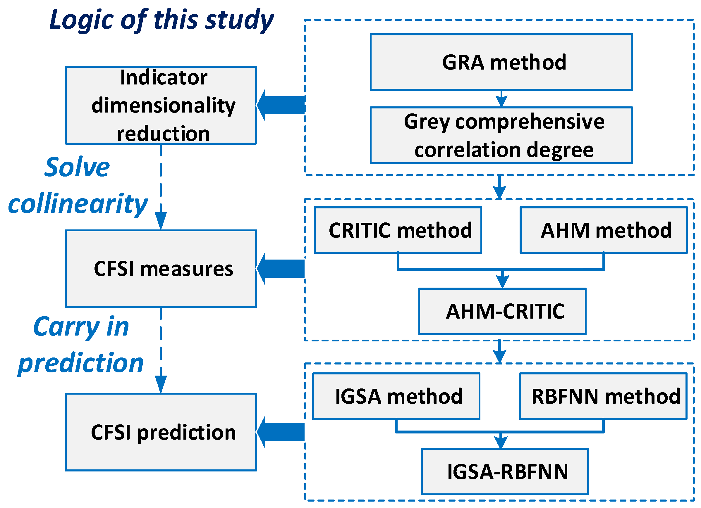
4. Methodology

In this chapter, a GRA-AHM-CRITIC coupling model and IGSA-RBFNN method will be introduced for the construction and prediction of the CFSI. The methodology framework is illustrated in Figure 1.

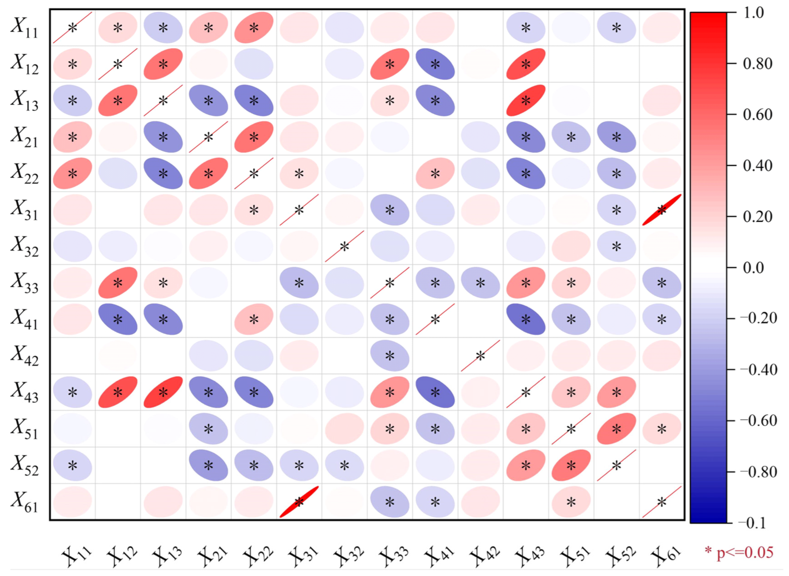
4.1. GRA Method

GRA theory was first proposed by Professor Deng in China in the 1980s [50]. GRA is a unified system that conducts quantitative analysis on each sequence, generating statistical datasets of the interrelationships between individual sequences and thereby determining their degree of correlation [51]. If the trend of change in the two series is more similar, the degree of association between these two series is higher, and vice versa.

Due to the co-movement of some economic variables and the inclusion of some lagged variables, multiple cointegration will be generated, thereby diminishing the significance of the indicator variables in the GARCH model [52]. Consequently, this could potentially undermine the predictive capability of the model, rendering its forecasts inconsequential. Therefore, to address the issues arising from cointegration and enhance the accuracy of series analysis results, GRA is used to calculate the comprehensive correlation between each indicator series, and the calculation steps are as follows.

Step 1: Define the reference sequence:

$$X_0(k)=\left[x_0(1),x_0(2),\cdots ,x_0(n_0)\right]$$

(8)

where $k=1,2,\cdots ,n_0$, where $n_0$ represents the number of sequences.

Step 2: Define the contrast sequence:

$$X_i(k)=\left[x_i(1),x_i(2),\cdots ,x_i(n_0)\right]$$

(9)

Step 3: Handling of variable dimensions: in order to mitigate the influence of variable dimensions in the original data, the dimensions of the variables in each raw data series should be calculated separately and then converted into a comparable series using a standardized formula:

$$X_i(k)=\frac{X_i(k)}{X_i(1)}$$

(10)

Step 4: Calculate the difference between the absolute value of the reference sequence and the comparison sequence:

$$V_i(k)=\left|X_0(k)-X_i(k)\right|$$

(11)

Step 5: Calculate the correlation coefficient between the reference series and the contrast series:

$${\xi }_i(x_0(k),x_i(k))=\frac{\underset{i}{min}\underset{k}{min}\left|x_0(k)-x_i(k)\right|+\rho \underset{i}{max}\underset{k}{max}\left|x_0(k)-x_i(k)\right|}{\left|x_0(k)-x_i(k)\right|+\rho \underset{i}{max}\underset{k}{max}\left|x_0(k)-x_i(k)\right|}$$

(12)

where $\rho$ is the resolution factor, taken as 0.5 [51].

Step 6: Calculate the degree of association:

$$r_i=\frac{1}{n{\displaystyle \sum _k^n\xi (k)}}$$

(13)

where r_i denotes the degree of correlation between the series; the larger the r_i value, the closer the relationship between the sequences.

4.2. Coupling Weight Calculation

4.2.1. AHM Method

AHM is a subjective assignment method. The proposed method, based on the Analytic Hierarchy Process (AHP) algorithm, offers several advantages including its wide applicability, ease of calculation, and consistency in testing. Furthermore, it inherits the strengths of AHP [53]. The specific empowerment steps for AHM are as follows:

Step 1: The weighting analysis of the evaluation indicators [54]. The Saaty scale is used to obtain the nth-order AHP discriminant matrix $K={\left(k_{ij}\right)}_{n\times n}$ by means of expert scoring, which $k_{ij}$ indicates the importance of the element i compared to the element j. AHP discriminant matrix $K={(k_{ij})}_{n\times n}$ properties are as follows:

$$\left\{\begin{array}{l}{k}_{ij}>0\\ k_{ii}=0\\ k_{ji}=1/k_{ij}\end{array}\right.$$

(14)

where $i\ne j,1\le i\le n,i\le j\le n$.

Step 2: Construction of the attribute discriminant matrix [55]. In the AHM, relative properties $l_{ij}$ form the nth order attribute discriminant matrix $L={\left(l_{ij}\right)}_{n\times n}$, where the relative attribute $l_{ij}$ and the scale $k_{ij}$ has the transformation relation in Equation (9).

$$l_{ij}=\left\{\begin{array}{l}2m/2m+1k_{ij}=m,i\ne j\\ 1/2m+1k_{ij}=1/m,i\ne j\\ 0.5k_{ij}=1,i\ne j\\ 0k_{ij}=1,i=j\end{array}\right.$$

(15)

where m denotes a positive integer greater than 2.

Step 3: Calculation of relative attribute weights between each indicator. From the AHM algorithm steps, the relative attribute weight $W_{AHM}$ between each indicator is calculated using Equation (10):

$$W_{AHM}=\frac{2}{n(n-1)}{\displaystyle \sum _{j=1}^n{l}_{ij}}$$

(16)

where $i=1,2,\cdots ,n$. n is the number of indicators and ${\displaystyle \sum _{i=1}^n{W}_{AHM}=1}$.

4.2.2. CRITIC Method

CRITIC is an objective weighting method that incorporates the influence of indicator variation size and the conflicting nature between indicators to determine weights in a more unbiased manner [56]. The conflicting nature of each evaluation indicator is determined based on the correlation of the indicators [57]. CRITIC’s specific empowerment steps are as follows:

Step 1: Calculate the standard deviation:

$${\sigma }_j=\sqrt{\frac{1}{m-1}{\displaystyle \sum _{i=1}^m{(x_{ij}-\overline{x_j})}^2}}$$

(17)

where $\overline{x_j}$ is the average of the indicators across the m programs and ${\sigma }_j$ is the standard deviation of $X_j$.

Step 2: Construct the correlation coefficient matrix:

$$r_{ij}=\frac{{\displaystyle \sum _{i=1}^n(x_i-\overline{x_i})(x_j-\overline{x_j})}}{\sqrt{{\displaystyle \sum _{i=1}^n{(x_i-\overline{x_i})}^2{\displaystyle \sum _{j=1}^n{(x_j-\overline{x_j})}^2}}}}$$

(18)

where $\overline{x_i}$ is the average of the schemes in index $X_i$ and $r_{ij}$ is the correlation coefficient between indicators $X_i$ and $X_j$.

Step 3: Find the combined weight of each indicator $W_{CRI}$:

$$s.t.\left\{\begin{array}{l}{W}_{CRI}=\frac{C_j}{{\displaystyle \sum _{i=1}^n{C}_j}}\\ C_j={\sigma }_j{\displaystyle \sum _{j=1}^n(1-r_{ij})}\end{array}\right.$$

(19)

where $C_j$ indicates the amount of information.

4.2.3. Lagrange’s AHM-CRITIC Coefficient Coupling

After determining the subjective weights W_AHM and objective weights W_CRI through AHM and CRITIC, the coupling weights through the Lagrange multiplier method are subsequently calculated to reflect the relative weight relationship of each indicator and its proportionate contribution within the entire framework [58]; the specific formula is as follows:

$$W_{AHM\_CRI}=\frac{{(W_{AHM}{W}_{CRI})}^{0.5}}{{\displaystyle \sum _{j=1}^n{(W_{AHM}{W}_{CRI})}^{0.5}}}$$

(20)

4.3. Prediction of the CFSI Using the IGSA-RBFNN

4.3.1. IGSA Method

Despite the availability of various algorithms, such as Particle Swarm Optimization (PSO) and Genetic Algorithm (GA), for optimizing model parameters, existing optimization methods are plagued by premature convergence and a lack of efficient acceleration mechanisms. The Gravitational Search Algorithm (GSA) is an innovative optimization algorithm inspired by the law of gravity. By employing a chaotic perturbation operator, GSA addresses these issues effectively, which has been utilized for parameter optimization in machine learning, as cited in [23]. To ensure that the FSI prediction model achieves higher predictive accuracy and generalizability, this study employs GSA to optimize three critical parameters in the RBFNN [59]: the number of nodes in the hidden layer C_j, the spread value σ_j, and the network connection weights ω_j. The optimization process ensures the reasonableness of the parameters and enhances the robustness of the predictions. The steps for constructing GSA are as follows.

In GSA, the agents are considered as mass-bearing objects [23]. These agents exert attractive forces on each other based on their masses, with the strength of attraction being directly proportional to their masses. Consequently, the agent with the largest mass is assumed to occupy the optimal position. Suppose there are N agents with a d-dimensional space. The position of the i-th agent can be expressed as follows:

$$X_i=(x_i^1,x_i^2,...,x_i^d)$$

(21)

At the t-th iteration, the force acting on the i-th agent originating from the j-th agent is defined as follows:

$$F_{ij}^d=G(t)\frac{M_i\left(t\right)M_j\left(t\right)}{R_{ij}\left(t\right)+\epsilon }(x_j^d(t)-x_i^d(t))$$

(22)

Here, $M_i\left(t\right)$ denotes the mass of the i-th agent, while $M_j\left(t\right)$ represents the mass of the j-th agent. G(t) is the gravitational constant at the t-th time, $\epsilon$ is a small constant, and $R_{ij}$ signifies the Euclidean distance between the i-th agent and the j-th agent. At the t-th iteration, the total force acting on the i-th agent is defined as follows:

$$F_i^d=\sum _{j=1,j\ne i}^{N}rand·F_{ij}^d\left(t\right)$$

(23)

where rand is a uniform random variable in the interval [0, 1]. In accordance with the law of motion, the acceleration of the agent at the t-th time can be expressed as follows:

$$a_i^d(t)=\frac{F_i^d}{M_i\left(t\right)}$$

(24)

In every iteration, the velocity and position of the i-th agent are updated using the following two equations:

$$v_i^d(t+1)=rand\times v_i^d\left(t\right)+a_i^d\left(t\right)$$

(25)

$$x_i^d(t+1)=x_i^d\left(t\right)+v_i^d(t+1)$$

(26)

where rand represents a uniform random variable in the interval [0, 1] and $x_i^d\left(t\right)$ and $v_i^d\left(t\right)$ are its current position and velocity. The conventional GSA, while effective in searching for algorithmic parameters in the RBFNN, exhibits relatively slow updates of gravitational coefficients and iteration speeds. In order to expedite this process, we propose an IGSA as a means to overcome these limitations [60]. The objective of IGSA is to enhance the gravitational coefficient, update speed formula, and position update formula of the regular GSA.

• Update of the gravitational coefficient [42]. The gravitational coefficient is enhanced through the utilization of a linear function, and the calculation formula can be seen in Equations (27) and (28).

  $$G\left(t\right)=G_0\left(1-t/T\right)$$

  (27)

  $$G_0=\gamma \underset{d\in \left|1,2,\cdots ,\left.n\right|\right.}{\max }\left(\left|x_{\max }^d-\right.\left.x_{\min }^d\right|\right)$$

  (28)
• Improved velocity $v_i^d$ update. By incorporating the memory function and population information sharing mechanism of the PSO algorithm [61], the GSA is improved. The improved spatial search method adopts a new strategy that not only adheres to the laws of motion but also increases the memory and population information communication mechanism. The new velocity update formula is defined as shown in Equation (29):

$$v_i^d(t+1)=ran{d}_i{v}_i^d(t)+a_i^d(t)+c_{1}ran{d}_j\left(p_b^d-x_i^d(t)\right)+c_{2}ran{d}_k\left(g_b^d-x_i^d(t)\right)$$

(29)

where rand_i, rand_j, and rand_k are random variables in the interval [0, 1]; c₁ and c₂ are constants in the interval [0, 1]; $p_b^d$ is the best position experienced by particle i; and $g_b^d$ is the best position experienced by all particles in the particle swarm. By fine-tuning the parameters of c₁ and c₂, the influence of gravity, memory, and population information on search can be balanced.

• Improved position $x_i^d$ update. The differential evolution algorithm employs a greedy selection mode, as depicted in Equation (30). When the fitness value of the new vector individual surpasses the fitness value of the target vector individual, the newly updated individual can be accepted by the population; otherwise, the individual of the previous generation will be retained in the subsequent generation population. Among them, the fitness value of the new position is lower than the fitness value of the previous generation position, leading to its replacement with the current generation’s position.

  $$x_i^d(t+1)=\left\{\begin{array}{l}ne{w}_i^t(t+1),f\left(ne{w}_i^t(t+1)\right)<f\left(x_i^d(t)\right)\hfill \\ x_i^d(t),otherwise\hfill \end{array}\right.$$

  (30)

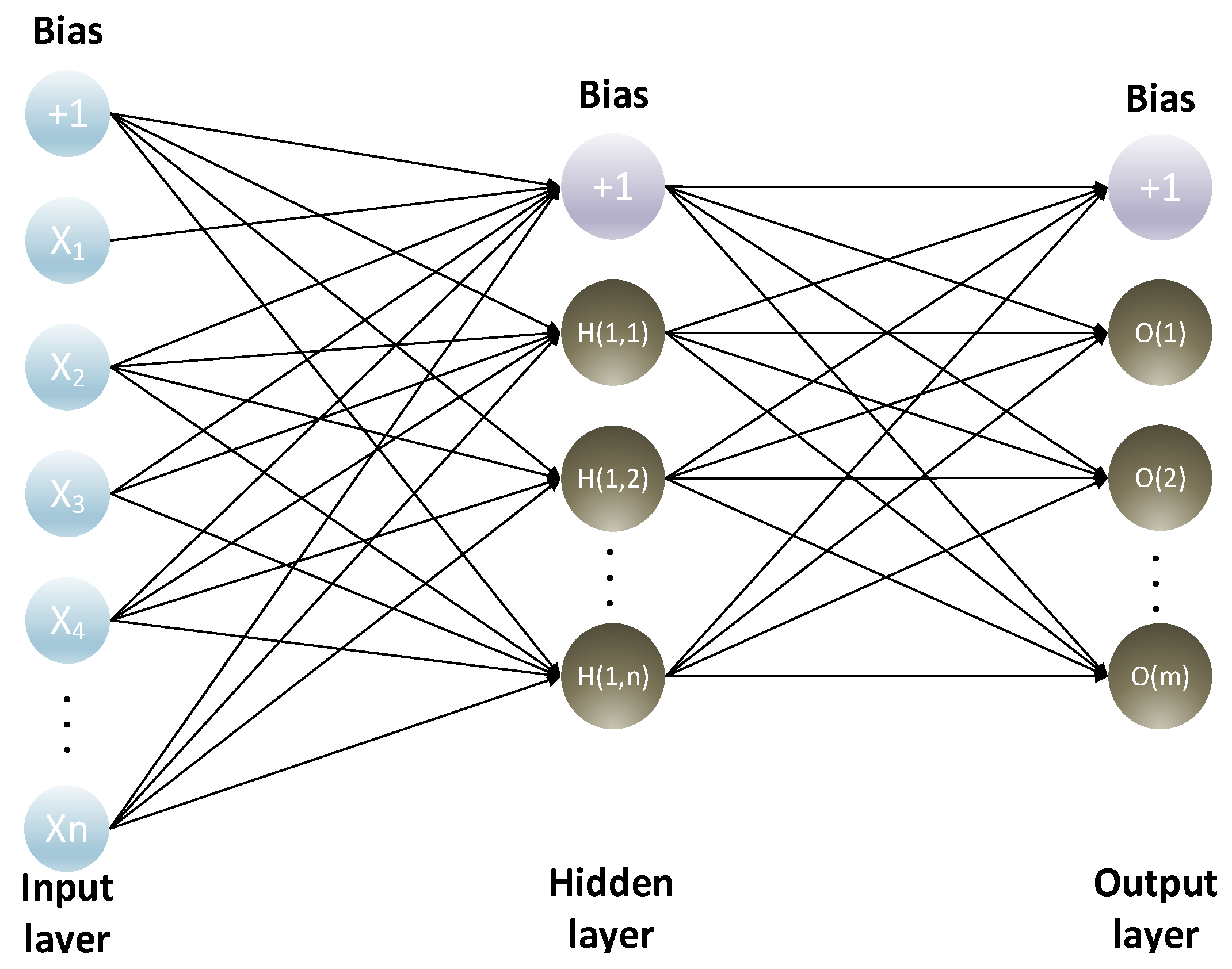
4.3.2. The RBFNN Method

The RBFNN is a type of feedforward neural network renowned for its fast learning speed and strong local approximation capability [41]. As shown in Figure 2, it is composed of an input layer, hidden layer, and output layer, with each output layer containing multiple neurons. Currently, the RBFNN finds extensive applications in domains such as pattern recognition, function approximation, time series prediction, and control systems [62]. The fundamental concept is to nonlinearly map the input space to a higher-dimensional feature space, allowing the model to tackle problems that are not linearly separable. In the hidden layer, the output of the j-th neuron is as follows:

$$Z_j(x)=exp(\frac{-{‖x-{\mu }_j‖}^2}{2{\sigma }_j^2})$$

(31)

where $x=\left[x_1,x_2,\cdots ,x_n\right]$ is an input; ${\mu }_j$ is the center of the j-th activation function; ${\sigma }_j$ is the parameter controlling the degree of smoothness of the activation function; and $‖x-{\mu }_j‖$ then indicates the Euclidean distance between the input and the functional center. The mapping function of the Gaussian activation function and the weighted linear summation in the common space in the output neuron of the RBFNN is illustrated as follows:

$$y={\displaystyle \sum _{j=1}^n{v}_j}{Z}_j(x)$$

(32)

where $Z_j(x)$ denotes the activation function of the j-th node, and $v_j$ then denotes the weight of the j-th node.

4.3.3. IGSA-RBFNN Prediction Model

In the learning process of an RBFNN, three main parameters need to be determined, namely the center of the hidden layer nodes’ basis functions $C_j$, the width value ${\sigma }_j$, and the network connection weight values $w_j$ [41]. In the optimized prediction model of the RBFNN, the crucial parameters are encoded into particles in the IGSA algorithm. The fitness value is defined as the coefficient of determination (R²) between the actual value and the predicted value [40]. Optimization is performed based on the gravitational interaction between individuals until the optimal individual is identified. The optimal individual obtained from the IGSA algorithm is utilized to assign values to the center $C_j$, width value ${\sigma }_j$, and network connection weight $w_j$ of the hidden layer nodes’ basis functions in the RBFNN, resulting in the IGSA-RBFNN prediction model [42]. The flowchart is shown in Figure 3.

4.3.4. Algorithm Accuracy Check

In the process of training and testing the artificial neural network, in order to obtain more accurate prediction results [63], the Mean Square Error (MSE) is utilized for evaluating the error during both testing and training phases of the neural network; the smaller the MSE value, the more accurate the prediction value of the neural network. The coefficient of determination R² is employed to evaluate the accuracy of the neural network in the prediction process. The range of values R² is between [0, 1]; the closer the value is to 1, the higher the accuracy of the neural network fit, and vice versa. The formula is as follows:

$$MSE=\frac{1}{n}{\displaystyle \sum _{j=1}^n{(t_j-y_j)}^2}$$

(33)

$$R^2=1-\frac{{\displaystyle \sum _{j=1}^n{(t_j-y_j)}^2}}{{\displaystyle \sum _{j=1}^n{(y_j)}^2}}$$

(34)

where t_j is the target value, y_j is the predicted value, and n is the number of data sets.

5. Result

5.1. Data Collection and Pre-Processing

Based on the WIND financial terminal, Guotaian database, People’s Bank of China and other databases and websites [64], quarterly, monthly and daily data were collected for a total of 15 indicators from January 2008 to December 2021 for six financial sub-markets in China, with descriptive statistics for each indicator as shown in

Table 2. Descriptive statistics of indicators.

Indicators	Max	Min	Mid	Mean
X11/CYN million	49,309.00	4415.00	15,479.50	16,231.43
X12/%	0.23	0.03	0.09	0.12
X13/%	6.69	0.80	2.27	2.30
X21/%	2.43	−0.62	1.23	1.09
X22/%	−0.03	−2.22	−0.67	−0.81
X31/%	0.04	0.01	0.02	0.01
X32/%	25.81	−25.85	0.44	0.26
X33	0.05	0.02	0.03	0.03
X41/%	0.02	0.00	0.01	0.01
X42/%	0.33	−0.22	−0.07	−0.01
X43	0.29	0.09	0.19	0.18
X51	1.67	0.02	0.75	0.76
X52/%	0.05	0.01	0.01	0.02
X61/%	−0.05	0.29	0.01	0.01

.

To address the issue of scale inconsistency, the indicators are initially categorized into two groups based on the evaluation pointers, and they are standardized based on the Max–Min method. The formula is shown in Equation (36):

$$x_{ij}^{\prime }=\frac{x_j-x_{min}}{x_{max}-x_{min}}$$

(35)

$$x_{ij}^{\prime }=\frac{x_{max}-x_j}{x_{max}-x_{min}}$$

(36)

where $x_{ij}^{\prime }$ is the value obtained after dimensionless processing of the original data and $x_j$ is the actual value of the indicator. Equation (35) is utilized for dimensionless treatment for the forward indicator and Equation (36) for the inverse indicator.

Based on the aforementioned data, Equations (15) to (20) are used to conduct grey correlation analysis on the collected data in order to mitigate issues such as lagged variable introduction and indicator prediction failure caused by multicollinearity [65].

Based on the GRA model constructed in Section 4.1, Figure 4 displays the grey relational matrix among various indicators with a dimensionality reduction threshold of 0.9 and significance testing at a p-value of 0.05 [66]. It can be seen that the correlation between indicators X₁₃ and X₄₃ reached 0.93; the correlation between indicators X₃₁ and X₆₁ reached 0.91; the X₃₁ and X₄₃ should be deleted as redundancy indicators [67].

5.2. CFSI Measurement

5.2.1. Calculation of AHM-CRITIC Weights

Despite previous research having explored the factors of instability in global financial markets, there remains a dearth of comprehensive evaluation concerning the interactions between these factors and their impact on market stress. To obtain a more exhaustive perspective, we invited 15 experts with extensive backgrounds in financial risk management. This group comprises of five finance professors from prestigious universities, five stock market experts, and five senior risk analysts from major global financial centers and regulatory agencies. These experts possess practical experience in areas such as financial market operations, policy formulation, asset risk assessment, and crisis response projects. By reviewing relevant literature on financial stress and incorporating insights from these experts, we constructed a scoring matrix encompassing key factors contributing to financial stress. This matrix not only reflects the impact of each factor on market stability but also elucidates their interrelations, thereby establishing a robust foundation for subsequent analysis.

The AHP discriminant matrix K (see

Table 3. AHP discriminant matrix K.

	X1	X2	X3	X4	X5	X6
X1	1	3	1	1/3	4	3
X2	1/3	1	1/2	1/4	1	3
X3	1	2	1	1/2	3	3
X4	3	4	2	1	5	4
X5	1/4	1	1/3	1/5	1	3
X6	1/3	1/3	1/3	1/4	1/3	1

) is constructed adopting expert scoring based on the Saaty scale, subsequently converted into the attribute discriminant matrix L (refer to

Table 4. AHM attribute discrimination matrix L.

	X1	X2	X3	X4	X5	X6
X1	0	6/7	1/2	1/7	8/9	6/7
X2	1/7	0	1/5	1/9	1/2	6/7
X3	1/2	4/5	0	1/5	6/7	6/7
X4	6/7	8/9	4/5	0	10/11	8/9
X5	1/9	1/2	1/7	1/11	0	6/7
X6	1/7	1/7	1/7	1/9	1/7	0

) through Equation (15). The AHP discrimination matrices for the sub-markets and the AHM attribute discrimination matrices are presented, respectively, in Appendix A and Appendix B. The construction of matrix eigenroots and eigenvectors or consistency test is unnecessary due to the attribute discrimination matrix’s consistent nature [68]. Attribute weights for each index are determined using Equation (16), yielding the overall weighting $W_{AHM}$ of the AHM model.

The CRITIC weighting method is employed to construct the correlation coefficient matrix through Equations ((17)~(19)), which in turn yields the weights of each indicator $W_{CRITIC}$, and the coupling of $W_{AHM}$ and $W_{CRITIC}$ is calculated using Equation (14). This gives the coupling weights $W_{AHM\text{-}CRITIC}$; the results are shown in

Table 5. Weighing outcomes and combining the weights of various approaches.

	AHM			CRITIC				${\mathit{W}}_{\mathit{A}\mathit{H}\mathit{M}\mathbf{\text{-}}\mathit{C}\mathit{R}\mathit{I}\mathit{T}\mathit{I}\mathit{C}}$
	${\mathit{W}}_{\mathit{A}\mathit{H}\mathit{M}\_1}$	${\mathit{W}}_{\mathit{A}\mathit{H}\mathit{M}\_2}$	${\mathit{W}}_{\mathit{A}\mathit{H}\mathit{M}}$	${\mathit{\sigma }}_{\mathit{j}}$	${\mathit{r}}_{\mathit{i}\mathit{j}}$	${\mathit{C}}_{\mathit{j}}$	${\mathit{W}}_{\mathit{C}\mathit{R}\mathit{I}\mathit{T}\mathit{I}\mathit{C}}$
$X_{11}$	0.19	0.11	0.02	0.21	10.63	2.18	0.09	0.04
$X_{12}$		0.31	0.06	0.15	10.81	1.63	0.06	0.06
$X_{13}$		0.58	0.10	0.22	11.56	2.49	0.10	0.10
$X_{21}$	0.10	0.75	0.08	0.22	9.41	2.03	0.08	0.08
$X_{22}$		0.25	0.03	0.23	8.73	1.98	0.08	0.05
$X_{32}$	0.20	0.75	0.15	0.16	9.17	1.51	0.06	0.10
$X_{33}$		0.25	0.05	0.14	9.04	1.24	0.05	0.05
$X_{41}$	0.37	0.75	0.28	0.29	11.62	3.33	0.13	0.20
$X_{42}$		0.25	0.10	0.33	10.38	3.43	0.13	0.12
$X_{51}$	0.09	0.17	0.02	0.16	11.03	1.81	0.07	0.04
$X_{52}$		0.83	0.07	0.20	13.40	2.63	0.10	0.09
$X_{61}$	0.06	1	0.06	0.12	10.82	1.33	0.05	0.06

, wherein $W_{AHM\_1}$ denotes the result of the assignment to each sub-market, $W_{AHM\_2}$ represents the individual weight assignments to indicators within their respective sub-markets, and $W_{AHM}$ signifies the weight of each indicator to the total market and is calculated as Equation (37)

$$W_{AHM}=W_{AHM\_1}\times W_{AHM\_2}$$

(37)

Table 5 indicates that indicator X₄₂ exhibits the highest combined weighting. In the process of assigning weights to this indicator, the AHM is considered as a subjective assignment method. The foreign exchange market in which indicator X₄₂ is located has a greater impact on the financial markets as a whole, and subjective weighting $W_{AHM}$ is greater than objective weighting $W_{CRITIC}$. While indicator X₁₃ receives the smallest combined weighting, it is noteworthy that the objective weights surpass the subjective weights in the process of assigning weights to the indicators, and the comparison demonstrates that the coupled weighting method can effectively weaken the effect of subjective extremes. The analysis of the objective weights reveals that there are three indicators (X₁₁, X₄₂, X₆₁) where the coupled weight $W_{AHM-CRITIC}$ exceeds the objective weight. This is also pertinent to the inherent conservatism of CRITIC’s mechanism, which exhibits limited responsiveness towards indicators with insignificant pressure changes, necessitating subjective weighting adjustments for optimal performance.

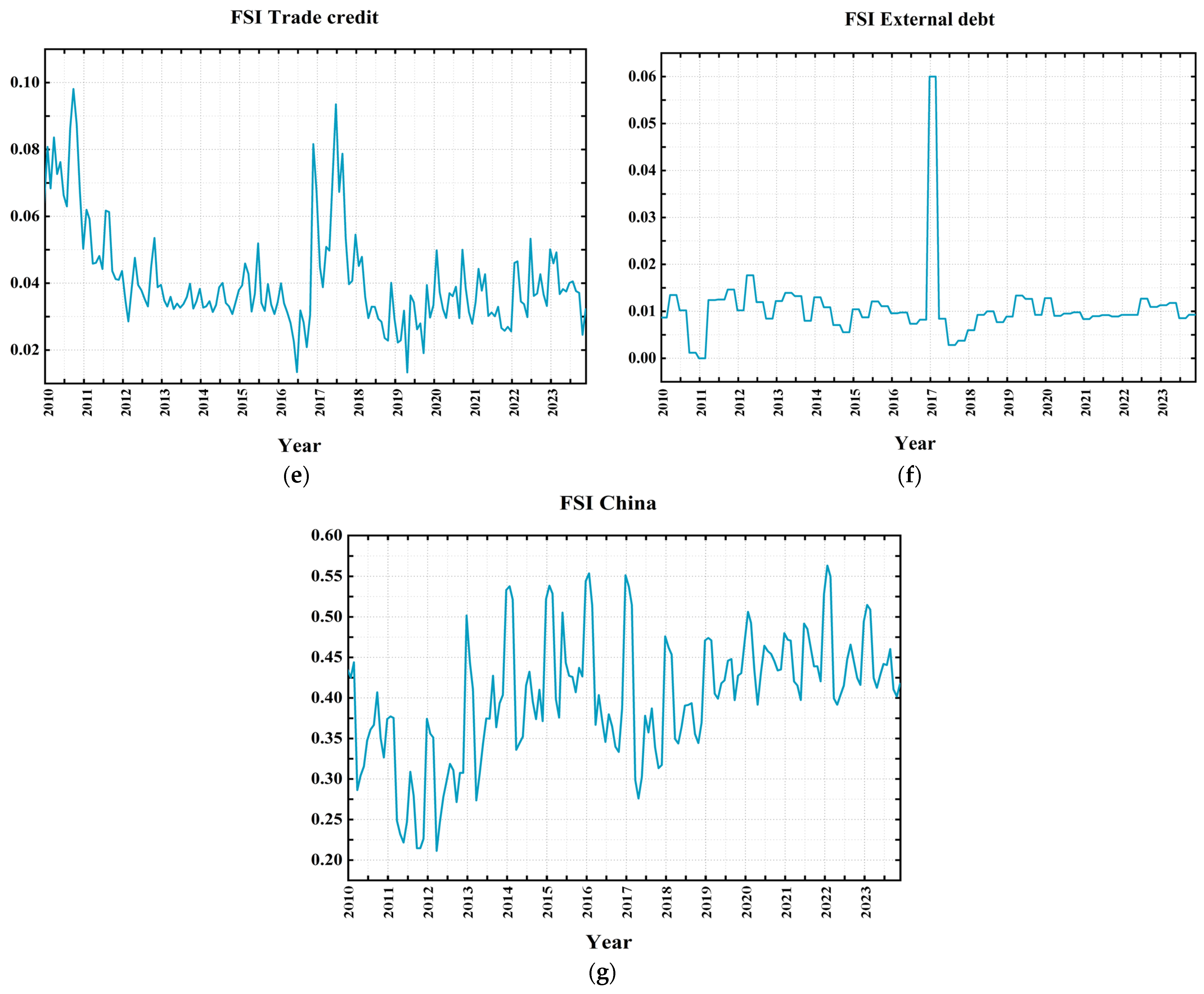
5.2.2. Trend Analysis of FSIs

The indexes are weighted according to the weights obtained from Equations (14)~(20) to obtain the financial stress indices of the money market (FSI Money), bond market (FSI Bond), stock market (FSI Stock), foreign exchange market (FSI Exchange), trade credit market (FSI Trade Credit) and external debt market (FSI External Debt), respectively. The financial stress indexes of six sub-markets, namely FSI Trade Credit, FSI External Debt, and FSI China, calculated according to Equation (7), are shown in Figure 4.

According to Figure 5a, China’s money market financial risk exhibits three stages of change: the first stage spans from January 2010 to February 2016. During this period, the global financial crisis in 2010 led to a significant increase in money market financial stress, reaching a peak value of 0.049 in November 2010. Subsequently, as a response to the crisis and an effort to alleviate money market financial stress, China implemented certain policies that resulted in a sharp decline, with the stress level dropping to a minimal value of 0.001 by February 2011. Following this decline, there was an oscillating rise in financial stress levels until it reached its maximum value of 0.09 by June 2015. The second stage, spanning from July 2015 to May 2017, witnessed a significant decline in financial stress within the money market as indicated by a peak value of 0.09 in May 2017. This reduction in financial risk can be attributed to various factors. Notably, the imposition of sanctions and tariffs on China by the United States in November 2016 potentially played a stabilizing role in the financial market [69] by incentivizing domestic production and curbing imports. Additionally, the Belt and Road Initiative (BRI) has also facilitated novel investment prospects and developmental opportunities in regions along its routes. This not only fosters economic growth in pertinent nations but also holds potential for mitigating financial risks. In light of these discoveries, it is recommended to continue implementing resilient risk management strategies, encompassing the utilization of tariffs and other trade policies, to uphold financial stability. Moreover, it is imperative to diligently monitor and address any potential risks and vulnerabilities that may arise in the financial market as a consequence of economic events and policy changes. The third stage is from June 2017 to December 2023, where the financial risk of the money market exhibits frequent oscillations, fluctuating between 0.017 and 0.071.

From Figure 5b, China’s bond market financial risk underwent three stages of change: January 2010 to June 2011 is the first stage, from 0.064 in January 2010 to 0.002 in June 2011; the reason is that the relatively safe bond market has become the “safe haven” of the nation. The second stage is from July 2011 to September 2013, during which China’s bond market developed steadily and expanded, and financial stress rose sharply from 0.016 in July 2011 to 0.116 in September 2013. The surge in financial stress during this phase can be attributed to the expansion of inter-bank liquidity and the subsequent escalation in inter-bank lending rates, which may have led to an augmentation of financial risk within the bond market. The intensified competition for funds among banks likely contributed to the adoption of risky lending practices and subsequently resulted in a surge in non-performing loans [70]. Therefore, it is imperative to persist in implementing robust risk management strategies, encompassing the vigilant monitoring and control of interbank liquidity, and adapting to fluctuations in interbank lending rates and other economic events so as to uphold financial stability. The third stage is from October 2013 to December 2023. The third stage is the period from October 2013 to December 2023, during which the financial stress in the bond market oscillates frequently, fluctuating between 0.056 and 0.121 overall.

From Figure 5c, it is evident that Chinese stock market financial risk undergoes four stages of change: the first stage spans from January 2010 to October 2010, characterized by a sharp increase in stock market financial stress due to the 2010 financial crisis, reaching an extreme value of 0.18 in October 2010; the second stage extends from November 2010 to June 2016, during which the stock market gradually stabilizes and experiences fluctuating levels of financial stress ranging between 0.072 and 0.148 overall; the third stage, spanning from July 2016 to April 2017, witnessed a period of stagnation in the Chinese stock market and a significant decline in stock market financial stress, with the latter decreasing from 0.106 in July 2016 to 0.037 in April 2017. The occurrence of Brexit has triggered a state of uncertainty in the global market, encompassing apprehensions regarding international trade relations [71]. This prevailing ambiguity may prompt investors to exercise caution in anticipation of an uncertain future, consequently exerting a detrimental influence on financial markets such as the Chinese stock market. Furthermore, the adjustment of the United States’ tariff policies towards China has resulted in an escalation of tariffs between the two nations, triggering a ripple effect within the global economy. The aforementioned pressure has exerted an impact on Chinese export businesses and manufacturing, thereby augmenting uncertainty within the global supply chain and precipitating a decline in the profitability of certain companies, consequently leading to a downturn in stock market performance. In such circumstances, investors tend to gravitate towards safer haven assets, thereby contributing to risk diversification within financial markets and mitigating portfolio volatility. May 2017 to December 2023 is the third stage, during which stock market financial stress oscillates frequently, fluctuating between 0.044 and 0.138 overall.

According to Figure 5d, China’s foreign exchange market financial risk exhibits an overall oscillating upward trend, characterized by a pronounced surge in financial stress at the onset of each year attributed to economic recovery and a robust but marginal increase in the external exchange rate. Subsequently, this period is followed by a deceleration in economic growth and a contraction of external spreads. In response to the economic cycle, enterprises and investors may exhibit an augmented demand for foreign exchange at the commencement of a new year, thereby contributing to market volatility. When economic growth decelerates, the external interest rate spread contracts, potentially alleviating financial strain. Additionally, heightened external interest rates can exert amplified financial pressure on the foreign exchange market [57], particularly for enterprises reliant on borrowing in foreign currencies. The fluctuations in the global economy exert a direct impact on the dynamics of the foreign exchange market. Due to the impact of the COVID-19 pandemic, the deceleration of the global economy has generated concerns regarding exchange rates, thereby exacerbating uncertainty in the foreign exchange market. The interplay of these factors gives rise to a multifaceted scenario wherein overall financial risk in the foreign exchange market exhibits an oscillating upward trajectory. Towards the end of the year, the market operates with enhanced efficiency and experiences reduced fluctuations in financial pressure. During the time interval from January 2010 to December 2023, values ranged from 0.194 in January 2010 to 0.174 in December 2023.

According to Figure 5e, the financial risk of China’s trade credit market exhibits three distinct stages of transformation: January 2010 to July 2016 is the first stage, during which the financial stress of the trade credit market oscillated down and reached a very minimal value of 0.018 in July 2016 for this period; the period from August 2016 to July 2017 represents the second stage, characterized by a notable upward trend in the trade credit market. The United Kingdom’s decision to leave the European Union in June 2016 led to a surge in global market uncertainty, with the progress and uncertainties surrounding Brexit negotiations exacerbating financial market volatility [71]. Consequently, this had an impact on the trade credit risks faced by multinational corporations. Additionally, in early 2017, the United States implemented a series of trade sanctions against China, sparking trade tensions between the two nations. This could have led to an escalation in financial risk in the trade credit market, affecting trade financing and credit conditions for businesses. The U.S.–China trade dispute and Brexit have introduced a heightened level of uncertainty into the global economy and trade system, exerting a direct impact on the trade credit market and reflecting the prevailing atmosphere of tension and unpredictability in global trade. The third stage is from August 2017 to December 2023, during which the financial risk in the trade credit market oscillates frequently, fluctuating between 0.013 and 0.079 overall.

According to Figure 5f, the financial risk in China’s external debt market exhibits three stages of change: January 2010 to November 2016 is the first stage, during which the trend of financial stress in the external debt market is relatively stable; the second stage, spanning from December 2016 to April 2017, witnesses a significant surge in financial risk within the bond market, with its value peaking at an impressive 0.45 in January 2017, after which it falls sharply and reaches a very small value of 0.06 in April 2017. Due to the United States implementing a series of trade sanctions against China in early 2017, it heightened the trade tensions between the U.S. and China. This likely contributed to an escalation in financial risk in the bond market [72], particularly in bonds associated with U.S.–China trade relations. Additionally, the uncertainty surrounding the Brexit negotiations may have exerted an impact on the bond market during this period. Concerns regarding the post-Brexit UK economy and financial markets might have prompted investors to re-evaluate bonds, thereby inducing fluctuations in financial risk. The substantial surge followed by a rapid decline in financial risk observed in the bond market during this period may imply a heightened level of market responsiveness to these events. There may have been instances of market overreactions or short-term hedging actions by participants due to uncertainties surrounding the subsequent developments of these events. May 2017 to December 2023 is the third stage, during which the financial risk in the bond market shows a relatively stable trend of 0.06. The third stage is from May 2017 to December 2023, during which the financial risk in the bond market shows a relatively stable trend.

According to Figure 5g, the seasonal pattern observed in China’s Financial Stress Index (FSI) is primarily due to macroeconomic cyclical changes within China’s financial market. Despite this, the characteristics of financial market risk show three stages of change: January 2010 to February 2016 is the first stage, during which China’s financial stress rose sharply and reached a very high value of 0.55 in February 2016; March 2016 to May 2017 is the second stage, during which China’s financial stress index fell sharply and reached a very high value of 0.27. The third stage spans from May 2017 to December 2023, during which China’s financial market risk experiences a significant surge and reaches a peak value of 0.42 in September 2023; apart from this, in each subsequent year, China’s financial market risk demonstrates an initial ascent followed by a subsequent descent, exhibiting pronounced upward trends at the beginning of the year and subsequently declining sharply.

The three aforementioned stages signify that despite the rapid and high-quality development of China’s financial market, there has been a dynamic intensification of potential risks and crises over the past decade [64]. In the initial phase (January 2010 to February 2016), the financial market encountered significant pressure stemming from repercussions from the global financial crisis and China’s economic structural adjustments. This period witnessed sharp market fluctuations and heightened pressure, indicating potential risks. The second stage (March 2016 to May 2017) may potentially reflect the favorable impacts of a series of macro-prudential policies and financial market reforms implemented by the Chinese government. The implementation of these policies might have contributed to mitigating financial risks and fostering market stability. The third stage (May 2017 to December 2023) may be susceptible to external influences, such as global economic uncertainty and trade tensions. This implies that China’s financial market is confronted with emerging potential risks in the recent period, necessitating heightened vigilance, monitoring, and responsive measures. Over the past decade, China’s financial market has undergone various stages of risks and crises, influenced by both global and domestic factors. The government has implemented effective policy measures to mitigate financial pressures corresponding to diverse economic conditions during different periods. Continued emphasis on monitoring global economic conditions and trade dynamics is strongly recommended. Moreover, it is imperative to prioritize prompt and adaptable policy responses to effectively tackle potential emerging economic and financial challenges.

5.3. FSI Prediction and Trend Analysis

After constructing the CFSI and its component indices, predictions for future financial stress index are conducted on the Python platform with a monthly time step, inferring fluctuations of each index over the next 48 periods. By employing the IGSA-RBFNN [73], we learned the FSI using data from 2010 to 2023. We randomly selected 70% of the data as the training set and 30% as the validation set. Based on this distribution, we conducted the algorithmic parameter settings. The number of IGSA-RBFNN neurons in the hidden layer is set to automatically iterate between 10 and 100, the learning rate is set to 0.1, number of iterations is set to 1000, and the L2 regularization rate is set to 1.0. In the IGSA optimization algorithm, the number of iterations is 150, c₁ = 0.15, c₂ = 0.25, G₀ = 100, and $\beta$ is 20. In addition, the RBF activation function and the Limited-memory Broyden Fletcher Goldfarb Shanno (L-BFGS) solver are used for computation [74]. Two evaluation metrics, R² and MSE, were employed to test the model performance.

The forecast results for 2024 to 2026 were obtained by forecasting the financial stress index of six financial market segments in China and the FSI of the total financial market in China through the IGSA-RBFNN, as shown in Figure 6a–g. The R² and MSE average levels are 0.9542 and 0.00023, respectively, indicating that the prediction model based on the IGSA-RBFNN has good robustness and generalization performance, suggesting that the prediction results are highly reliable.

According to Figure 6a, China’s money market faces three distinct phases of future financial risk. The initial phase, spanning from January 2024 to June 2024, demonstrates a noteworthy escalation in risk, indicating potentially volatile economic conditions. The observed risk exhibits an upward trend, with a gradual increase from 0.039 in January 2024 to 0.052 in June 2024, indicating the necessity for enhanced vigilance and potential adjustments to risk management strategies among market participants. The second stage spans from July 2024 to January 2025 and represents a period of stabilization in the market. Relevant stakeholders, including investors and regulators, should judiciously capitalize on this phase by implementing prudent measures [10] such as fortifying liquidity buffers or reassessing interest rate policies to effectively mitigate any forthcoming risks. The third stage, lasting from February 2025 to February 2026, is characterized by frequent oscillations in financial risk levels. In December 2025, the financial risk reaches its peak at 0.052, followed by significant fluctuations ranging between 0.005 and 0.058 from January 2026 to December 2026. Given the persistent volatility, it is imperative to conduct a comprehensive evaluation of existing investment portfolios and implement more robust hedging techniques in order to mitigate potential market fluctuations.

The financial risk trajectory of China’s bond market, as shown in Figure 6b, goes through three distinct stages. Initially, from January 2004 to October 2024, the bond market experiences an oscillating yet ascending pattern of financial risk, increasing from 0.069 in November 2024 to 0.093 in October 2024. This period is characterized by heightened market volatility, necessitating increased regulatory and investor scrutiny to anticipate potential adjustments and establish robust risk management protocols [52], reinforcing market confidence and curbing speculation. In the second stage from November 2024 to May 2025, there is a noticeable decline in financial risk, decreasing from 0.083 to 0.077. This substantial decline provides a cautiously optimistic outlook for policy adjustments and investment prospects. During the final stage from June 2025 to December 2026, the bond market experiences frequent fluctuations in financial risk, ranging between 0.073 and 0.105. This uncertain period underscores the potential impact of both domestic and international developments on market stability. Market participants should utilize this phase to evaluate their risk diversification strategies and operational frameworks’ responsiveness to sudden shifts, strengthening financial security amidst continuous market changes.

The projected stages of financial risk in China’s stock market, as shown in Figure 6c, indicate a nuanced trajectory over the next three years. In the initial phase (January 2024 to July 2024), there is a gentle downtrend in financial risk from 0.121 to 0.091. The observed decline implies a state of relative stability, thereby reflecting favorably on the current financial policies and risk management practices. It is imperative to uphold and potentially reinforce these measures in order to sustain the positive momentum. During the second stage from August 2024 to October 2025, the stock market experiences increased volatility, with fluctuations mainly ranging between 0.081 and 0.099. Measures like enhanced market surveillance, real-time monitoring of macroeconomic indicators, and adaptive policy frameworks could be considered to manage unpredictable swings and boost investor confidence. The final stage, spanning from November 2025 to December 2026, sees a gradual decline in financial risk, reaching 0.073 by the end of this period. This descent indicates the maturation of market mechanisms and the adaptation of investors to previous regulatory measures, while harnessing advancements in predictive analytics could proactively address risk factors and formulate effective strategies.

According to Figure 6d, in the initial phase from January 2024 to October 2025, there is a gradual decline in financial risk, signaling stabilization with a decrease from 0.237 to 0.157. The observed phenomenon can be ascribed to the implementation of effective regulations and the presence of a favorable global economic climate. The subsequent period, from November 2025 to February 2026, witnesses a sharp increase in financial risk levels, with the risk soaring back to its peak of 0.237. This surge may potentially reflect the market’s response to unforeseen internal or external shocks like geopolitical tensions, sudden economic policy shifts, or global market volatility. It underscores the necessity for robust contingency plans and flexible monetary policies that can promptly address unexpected financial strain. In the final stage, from March 2026 to December 2026, the financial risk in the foreign exchange market sharply declines to 0.171. This reduction may indicate successful implementation of mitigation strategies and adaptive mechanisms by the market to handle the mentioned shocks.

According to Figure 6e, China’s trade credit market financial risk is expected to undergo a three-phase evolution in the near future. The initial phase, from January 2024 to May 2025, shows a gradual increase in financial risk, with the trade credit market risk index rising from 0.037 to 0.056. The findings imply a state of relative stability; however, it is crucial to exercise cautious monitoring in order to prevent any potential disruptive escalation that may adversely affect market confidence. The second phase, from June 2025 to November 2025, sees a sharp increase in the risk index, reaching a peak of 0.067. Reinforced oversight, encompassing meticulous examination of trade credit transactions and adherence to stringent credit standards, could prove pivotal in averting potential defaults stemming from excessive leverage. The final stage, from December 2025 to December 2026, is characterized by frequent oscillations in financial risk levels ranging from 0.023 to 0.041. This period of volatility underscores the imperative for the need for robust risk management frameworks and sufficient market liquidity to absorb unexpected shocks. Exploring diversification of trade finance products across sectors and regions can effectively distribute risk more evenly.

According to Figure 6f, the financial risk of China’s external debt market undergoes three stages of change. In the first stage, from January 2024 to October 2025, the financial risk of the external debt market exhibits a slow decline, from 0.009 in January 2024 to 0.007 in October 2025, it is still a crucial period for maintaining the stability of the external debt market. In the second stage, from November 2025 to April 2026, there is a notable surge in the financial risk observed within the external debt market, climbing from 0.008 in January 2025 to 0.012 in April 2026. The escalation in financial risk may be linked to economic uncertainty and shifts in global politics. To mitigate these risks, we propose enhancing external debt transparency, promoting international financial stability through heightened cooperation among nations [13]. In the third stage, from May 2026 to December 2026, the financial risk in the external debt market shows a sharp decrease, falling from 0.012 in April 2026 to 0.01 in December 2026. The sharp decline in financial risk may create potential opportunities for external debt investment. It is recommended to optimize the structure of external debt investments, diversify the portfolio, and foster the healthy development of the external debt market.

According to the analysis of data presented in Figure 6g, China’s financial market risk is expected to undergo four stages of change. In the first stage from January 2024 to November 2024, the overall financial market risk is predicted to exhibit a substantial decline from 0.548 in January 2024 to 0.421 in November 2024, followed by a short period of fluctuation. Reputable financial institutions should leverage favorable market conditions to enhance their capitalization, fortify risk management capabilities, and proactively prepare for potential escalations in financial risks during subsequent stages [46]. The second stage runs from December 2024 to February 2025, during which the financial market risk is projected to increase rapidly from 0.426 in December 2024 to 0.543 in February 2025. Reputable financial institutions should adopt a prudent investment approach and refrain from excessive borrowing in order to mitigate the risks of credit defaults. The third stage spans from March 2025 to September 2026, where the financial market risk is expected to rise sharply from 0.548 in January 2024 to a peak of 0.53 in September 2026 with a slow upward trend. The regulators should enhance market surveillance, closely monitor the conduct of financial institutions, and implement macroprudential measures to prevent systemic risks. The fourth stage occurs from October 2026 to December 2026, where the financial market risk is forecast to experience a significant drop from 0.530 in October 2026 to 0.467 in December 2026. The prompt and effective implementation of support measures, such as the injection of liquidity, is imperative for stabilizing financial markets and fostering sustainable economic growth.

6. Conclusions and Prospect

6.1. Conclusions and Suggestions

Despite the absence of overt signs of severe financial crises, the ongoing transition process towards a market economy remains incomplete within the context of still developing emerging markets. The disparities in the reform of local and global financial systems give rise to significant financial volatility, underscoring the imperative for establishing a timely FSI. The sub-indices derived from the analysis conducted in this study illustrate how market volatility and uncertainty can potentially impact the overall market dynamics, particularly during economic downturns, thereby exerting influence on long-term growth trends. The predictive efficacy of the financial stress index has been empirically validated, thereby enabling proactive measures to mitigate adverse financial events and facilitating timely interventions. The research findings suggest that factors inherent in transitional systems may give rise to significant financial volatilities, potentially precipitating subsequent financial crises. Therefore, based on the comprehensive evaluation and prediction results of the CFSI as well as studies on relevant major financial events, specific recommendations are proposed.

• Building a timely risk warning system is crucial for curbing systemic risks in financial markets. Despite the availability of adequate qualitative analysis on such risks, there is a noticeable dearth of quantitative analysis and mathematical support [75]. The inadequacy is also apparent in the imperfect mechanisms for early warning of financial risks. As evidenced by the forecast results of the CFSI, there is a gradual and consistent increase in the CFSI from 2024 to 2026. Therefore, it is imperative to develop dedicated early warning models to enhance the resilience level of systemic risks.
• The interaction among financial subsystems can engender instability in the overall market. For instance, the financial risk of the Chinese bond market rose from 0.064 in 2010 to 0.002 in 2011 and subsequently increased to 0.116 during a stable expansion period. According to model predictions, the expected range of bond financial risk is projected to fluctuate between 0.073 and 0.105 from 2024 to 2026. Moreover, the risk level in the money market has witnessed an upward trend over recent years, increasing from a minimum of 0.001 to a maximum of 0.071, and it is anticipated to oscillate within the range of 0.052 and 0.058 during the period spanning from 2024 to 2026. Therefore, it is imperative to enhance the scope, frequency, and quality of microeconomic financial data collection to effectively mitigate risk propagation across multiple subsystems and aggregate statistical risk indicators, thereby safeguarding investor interests.
• The ongoing financial reform in China is gradually aligning with the transformation of its economic structure, exemplified by measures implemented in special economic zones as well as agricultural and industrial reforms. However, these reforms lack alignment with global financial issues, potentially leading to distortions in the pricing structure of capital markets and an escalation of stability risks within the financial system. Running through the financial system reforms is the foreign exchange market, which fluctuated from 0.194 in 2010 to 0.174 in 2023. The projected pace of reform is expected to raise this figure to 0.237 in 2024 and then decrease to 0.171 by the end of 2026. China should carefully calibrate the pace and extent of its reforms to ensure a seamless transition of the financial system, while striking an optimal equilibrium between fostering long-term reforms and maintaining stability.
• Given the extensive experience of the international P2P lending model, it is imperative to re-evaluate the issue of ‘rigid redemption’ in the Chinese market and implement prompt measures for its resolution. Due to a substantial influx of funds into the net lending sector, the real sector is encountering challenges in securing adequate financing for its expansion, thereby necessitating prioritization of liquidity issues arising from inflexible redemption policies [76]. For example, the risk in the external debt market peaked at 0.45 in January 2017 but then fell to 0.06 in April of the same year. Forecasts show that this market will remain relatively stable from 2024 to 2026. Therefore, it is imperative to eliminate the policy of “principal and interest guarantee” for P2P lending products and guide investors towards enhancing their risk awareness. This will enable investors to assume the risks themselves, thereby alleviating the burden on the entire online lending industry.

6.2. Comparison Analysis

To better illustrate the robustness and generalization performance of the IGSA-RBFNN algorithm in the CFSI, this study selects algorithms such as the Multi-Layer Perceptron Neural Network (MLPNN), RBFNN, Light Gradient Boosting Machine (LightGBM), and GSA-RBFNN for algorithm comparison, which are used for parameter accuracy testing, and their MSE and R² results are shown in Figure 7 and Figure 8.

The collected data were trained using five different algorithms to test the accuracy on the CFSI, MFSI, BFSI, EFSI, TCFSI, and FDFSI. According to Figure 7 and Figure 8, it is concluded that the IGSA-RBFNN algorithm has an average MSE of 0.0002 and an average R² of 0.9629. Meanwhile, the MSE results obtained from the LightGBM, MLPNN, and RBFNN algorithms fluctuate between 0.0009 and 0.0026, with R² results fluctuating between 0.9383 and 0.9513. The average MSE and average R² of the GSA-RBFNN algorithm are 0.0009 and 0.9547, respectively.

Comparing the accuracy testing results of each algorithm indicates that the precision tests conducted on the IGSA-RBFNN algorithm are superior to other algorithms, with the GSA-RBFNN algorithm following closely behind. The accuracy testing results of the LightGBM, MLPNN, and RBFNN algorithms are slightly inferior. This suggests that the IGSA-RBFNN algorithm exhibits better robustness and applicability to the mechanisms influencing financial risk and indices of financial risk, reflecting superior predictive performance, generalization capabilities, and resistance to overfitting compared to similar algorithms.

7. Conclusions and Prospect

7.1. Conclusions

The systematic method of constructing and calibrating financial system stress measurement for the CFSI measurement process is explained. The CFSI plays a pivotal role in the surveillance of financial risk in China, providing an effective approach to employing financial instruments for gauging the stress on the financial system. The outcomes of this stress measurement reflect the relative contributions of individual indicators towards overall pressure. From an economic policy standpoint, implementing appropriate economic measures during times of financial stress depends on identifying and addressing the root causes behind such stress. If the primary source of financial strain lies within the bond market, it becomes imperative for economic policies to prioritize bolstering and fortifying this particular market segment. The measurement of financial stress is thus valuable in assisting policymakers to formulate appropriate economic policies for addressing financial risks. The primary conclusions are as follows:

(1)

In the process of measuring the CFSI, we meticulously considered the unique characteristics of China as a developing nation and comprehensively explored the information quality of each indicator. The final CFSI encompasses six major market segments: currency, bond, stock, foreign exchange, trade credit, and foreign debt markets. Additionally, it evaluates the overall financial risk in China and its associated risks within these six major segments. The financial stress between 2010 and 2023 basically shows three stages of change, with financial stress shaking out and rising from January 2010 to February 2016, falling sharply from March 2016 to May 2017, and rising sharply from May 2015 to December 2023; the overall financial risk is relatively high.

(2)

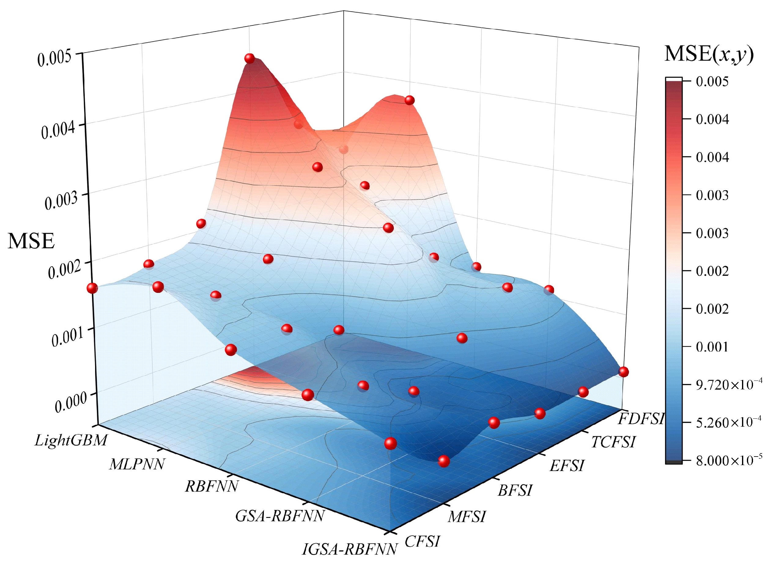
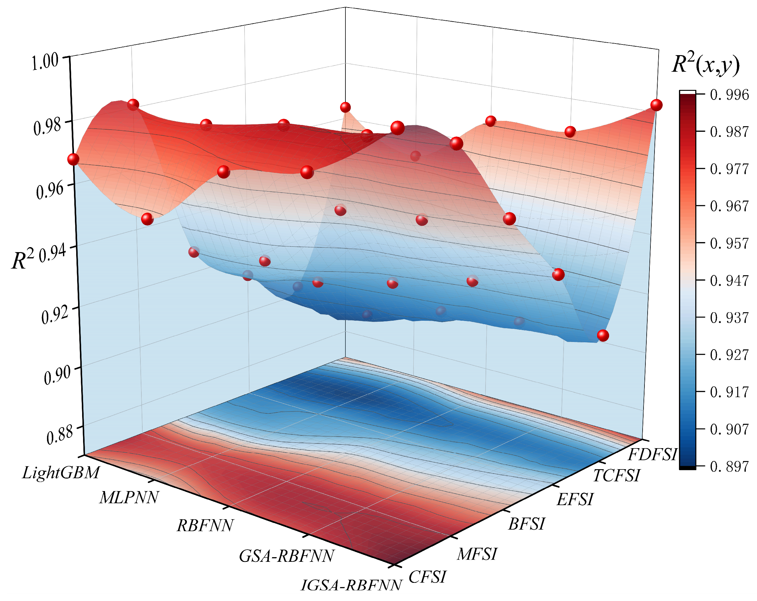
In the process of forecasting the CFSI, the IGSA-RBFNN is utilized to forecast the financial stress index for the years 2024 to 2026. Additionally, the MSE is employed to test the accuracy of the algorithm, ensuring the validity of the forecast results. The forecast results indicate that the overall financial market and six major market segments in China have a lower level of financial risk from July 2025 to January 2026 compared with other periods, while the Chinese financial system is in a long-term high-stress stage from January 2026 to August 2026, indicating that economic activities are relatively frequent during this period.

7.2. Limitations and Future Work

This article utilizes the GRA, AHM-CRITIC and IGSA-RBFNN model to conduct out-of-sample predictions of the CFSI in order to accurately evaluate China’s systemic financial risks, which play a crucial role in maintaining stability within its financial markets. However, it is essential to address certain limitations in future research endeavors.

(1)

In the GRA, the correlation between indicators is mitigated by implementing a stringent correlation coefficient threshold of 0.9. The selection of different thresholds may exert an impact on the final outcomes, and future investigations could conduct additional sensitivity analyses to ascertain the optimal threshold.

(2)

For the long-term prediction of CFSI trends, there are numerous uncertainties encompassing political, economic, and social dynamics that may potentially hinder the accuracy of the model. The proposed forecasting model is based on sample data from 2010 to 2023, which is used to predict the trends of the CFSI for the subsequent 48 months. The model demonstrates a certain level of timeliness and can be further developed into a dynamic forecasting model that incorporates new data in order to apply the predictive framework to other countries and regions.

(3)

Although this article presents the effective prediction of the FSI using the IGSA-RBFNN algorithm, it lacks empirical research on the dynamic relationship between financial risk factors. In the future, to achieve efficient risk prediction and control, it is possible to further employ advanced methodologies such as Structural Equation Modeling (SEM), the System Dynamics Method (SDM) [77,78], and other systems theory models for exploring the generation and dynamic evolution analysis of financial stress.

References

- Al-Fayoumi, N.; Abuzayed, B.; Arabiyat, T.S. The banking sector, stress and financial crisis: Symmetric and asymmetric analysis. Appl. Econ. Lett. 2019, 26, 1603–1611. [Google Scholar] [CrossRef]
- Koomson, I.; Churchill, S.A.; Munyanyi, M.E. Gambling and Financial Stress. Soc. Indic. Res. 2022, 163, 473–503. [Google Scholar] [CrossRef]
- Chiba, A. Financial Contagion in Core–Periphery Networks and Real Economy. Comput. Econ. 2020, 55, 779–800. [Google Scholar] [CrossRef]
- Chen, X.R.; Hao, A.M.; Li, Y.L. The impact of financial contagion on real economy-An empirical research based on combination of complex network technology and spatial econometrics model. PLoS ONE 2020, 15, e229913. [Google Scholar] [CrossRef]
- Keda, W. Research on the Construction of Financial Stress Index and Its Macroeconomic Effects. Shanghai Financ. 2020, 1, 30–38. [Google Scholar] [CrossRef]
- Wen, Z. China’s Growth Accounting Based on Binary Structure: Theoretical and Empirical Analysis of Introducing Labor Employment Rate. Soc. Sci. China 2023, 39–58. [Google Scholar]
- Huang, X.; Guo, F.Y. A kernel fuzzy twin SVM model for early warning systems of extreme financial risks. Int. J. Financ. Econ. 2021, 26, 1459–1468. [Google Scholar] [CrossRef]
- Li, C.; Zhao, Y.T. A Study on the Linkage of Leverage Ratio, Real Estate Prices, and Financial Risks in Various Sectors of the Real Economy. Financ. Regul. 2021, 3, 92–114. [Google Scholar] [CrossRef]
- Yang, H. Construction and Analysis of China’s Systemic Financial Risk Stress Index. West. Financ. 2019, 6, 38–42. [Google Scholar] [CrossRef]
- Ahamed, M.M. Inclusive banking, financial regulation and bank performance: Cross-country evidence. J. Bank. Financ. 2021, 124, 106055. [Google Scholar] [CrossRef]
- Illing, M.; Liu, Y. Measuring financial stress in a developed country: An application to Canada. J. Financ. Stabil. 2006, 2, 243–265. [Google Scholar] [CrossRef]
- Yang, L.X.; Lin, J.Y.; Meng, S.S. China Financial Stress Index and Monitoring Efficiency Evaluation. Shanghai Econ. Res. 2024, 1, 106–120. [Google Scholar] [CrossRef]
- Tan, Z.M.; Wang, X.; Yang, S.M. Research on the Cross Market Transmission of Systemic Financial Risks Based on Stress Index. Econ. Forum 2023, 7, 139–152. [Google Scholar]
- Xu, D.Q. On the Regulatory Failure and Tax Regulation of Systemic Financial Risks. Political Leg. Theory Ser. 2024, 1, 14–28. [Google Scholar]
- Cevik, E.I.; Dibooglu, S.; Kenc, T. Financial stress and economic activity in some emerging Asian economies. Res. Int. Bus. Financ. 2016, 36, 127–139. [Google Scholar] [CrossRef]
- Wu, G.L.; Wu, X.T.; Wang, B. Analysis of the impact of the COVID-19 on China’s systemic financial risks: Based on the financial stress index and portfolio model. Manag. Mod. 2021, 41, 103–107. [Google Scholar] [CrossRef]
- Tiwari, A.K.; Nasir, M.A.; Shahbaz, M. Synchronisation of policy related uncertainty, financial stress and economic activity in the United States. Int. J. Financ. Econ. 2021, 26, 6406–6415. [Google Scholar] [CrossRef]
- MacDonald, R.; Sogiakas, V.; Tsopanakis, A. Volatility co-movements and spillover effects within the Eurozone economies: A multivariate GARCH approach using the financial stress index. J. Int. Financ. Mark. Inst. Money 2018, 52, 17–36. [Google Scholar] [CrossRef]
- Zheng, K.Y.; Xiang, X.H. Water Quality Evaluation Model of Xiaoxingkai Lake Based on AHM-CRITIC Weighting. Water Sav. Lrrigation 2020, 9, 79–83. [Google Scholar] [CrossRef]
- Xiao, H.Y.; Zhen, Z.Y.; Xue, Y.X. Fault-tolerant attitude tracking control for carrier-based aircraft using RBFNN-based adaptive second-order sliding mode control. Aerosp. Sci. Technol. 2023, 139, 108408. [Google Scholar] [CrossRef]
- Li, J.Z.; Wang, M.C. How modern financial support drives innovative urban planning and construction: Grey relation analysis. Open House Int. 2018, 43, 118–123. [Google Scholar]
- Liu, B.W.; Dong, L.; Fan, R.Z. In Research on the financial risk measurement and prediction of small and medium-sized enterprises based on the artificial neural network under AHM-CRITIC coupling. In Proceedings of the 2022 International Conference on Agriculture, Forestry and Economic Management (AFEM 2022), Shanghai, China, 28 May 2022. [Google Scholar]
- Salim, A.; Irman; Hadimi; Hardiansyah. Hybrid PSO-GSA Applied To Dynamic Economic Dispatch With Prohibited Operating Zones. IOSR J. Electr. Electron. Eng. 2019, 1, 10–17. [Google Scholar]
- Balakrishnan, R.; Danninger, S.; Elekdag, S.; Tytell, I. The Transmission of Financial Stress from Advanced to Emerging Economies. Emerg. Mark. Financ. Trade 2011, 47, 40–68. [Google Scholar] [CrossRef]
- Yao, X.Y.; Le, W.; Sun, X.L.; Li, J.P. Financial stress dynamics in China: An interconnectedness perspective. Int. Rev. Econ. Financ. 2020, 68, 217–238. [Google Scholar] [CrossRef]
- Li, S.; Liu, X.X. Financial systemic stress: Index construction and spillover effect measurement. Syst. Eng.-TheoryPract. 2020, 40, 1089–1112. [Google Scholar]
- Babar, S.; Latief, R.; Ashraf, S.; Nawaz, S. Financial Stability Index for the Financial Sector of Pakistan. Economies 2019, 7, 81. [Google Scholar] [CrossRef]
- Dai, B.B.; He, W.J. An Empirical Study on the Construction of China’s Financial Stress Index and Economic Warning. Financ. Theory Pract. 2018, 39, 27–32. [Google Scholar] [CrossRef]
- Yao, X.Y.; Sun, X.L.; Li, J.P. The Construction Method and Empirical Study of China’s Financial Stress Index Considering Market Correlation. Manag. Rev. 2019, 31, 34–41. [Google Scholar] [CrossRef]
- Xu, G.X.; Li, B. Research on the Construction and Dynamic Transmission Effect of China’s Financial Stress Index. Stat. Res. 2017, 34, 59–71. [Google Scholar] [CrossRef]
- Yang, L.S.; Yang, J. Research on the time-varying nonlinear effects of financial pressure spillovers on macroeconomics. Manag. Mod. 2022, 42, 58–64. [Google Scholar] [CrossRef]
- Ilesanmi, K.D.; Tewari, D.D. Financial Stress Index and Economic Activity in South Africa: New Evidence. Economies 2020, 8, 110. [Google Scholar] [CrossRef]
- Kim, H.; Shi, W.; Kim, H.H. Forecasting financial stress indices in Korea: A factor model approach. Empir. Econ. 2020, 59, 2859–2898. [Google Scholar] [CrossRef]
- Chen, Z.Y.; Xu, Y. Research on the Construction and Application of China’s Financial Stress Index. Contemp. Econ. Sci. 2016, 38, 27–35. [Google Scholar]
- Ding, H.; Chen, Y.; Bian, Z.C. Construction of China’s Financial Market Stress Index and Its Macroeconomic Nonlinear Effects. Mod. Financ. Econ.-J. Tianjin U 2020, 40, 18–30. [Google Scholar] [CrossRef]
- Sahoo, J. Financial stress index, growth and price stability in India: Some recent evidence. Transnatl. Corp. Rev. 2021, 13, 222–236. [Google Scholar] [CrossRef]
- Zhang, K.X. Construction and analysis of regional financial pressure index. North China Financ. 2019, 03, 57–61. [Google Scholar]
- Xu, Y. A Study on the Effectiveness of Systematic Stress Composite Index. Stat. Decis. 2017, 02, 166–170. [Google Scholar] [CrossRef]
- Bai, L.B.; Wang, Z.G.; Wang, H.L.; Huang, N.; Shi, H.J. Prediction of multiproject resource conflict risk via an artificial neural network. Eng. Constr. Archit. Manag. 2021, 28, 2857–2883. [Google Scholar] [CrossRef]
- Zhang, S.; Chen, X.H.; Liu, Q.; Liu, Z.; Wang, Q.L. Coupling PSO and Extended RBF Neural Network to Estimate the ZTD Calculation Accuracy of NWM Model. Acta Geod. Et Cartogr. Sin. 2022, 51, 1911–1919. [Google Scholar]
- Zhang, J.C.; Zhang, Z.C.; Hou, J.X. Monitoring method for gasification process instability using BEE-RBFNN pattern recognition. Int. J. Hydrog. Energ. 2021, 46, 16202–16216. [Google Scholar] [CrossRef]
- Jajam, N.; Challa, N.P.; Prasanna, K.S.; Prasanna, K.S.; Ch, V.S. Arithmetic Optimization with Ensemble Deep Learning SBLSTM-RNN-IGSA model for Customer Churn Prediction. IEEE Access 2023, 11, 93111–93128. [Google Scholar] [CrossRef]
- Zhou, R.; Wang, X.; Mei, Y. An Optimization Model of Static Term Structure of Interest Rates Based on the Combinatorial Forecast Method. Oper. Res. Manag. Sci. 2014, 23, 205–212. [Google Scholar]
- Zheng, B.C. Financial default payment predictions using a hybrid of simulated annealing heuristics and extreme gradient boosting machines. Int. J. Internet Technol. Secur. Trans. 2019, 9, 404–425. [Google Scholar] [CrossRef]
- Ling, T.; Ying, Z. Monitoring and Measurement of Systemic Financial Risks: A Study Based on China’s Financial System. J. Financ. Res. 2016, 6, 18–36. [Google Scholar]
- Apostolakis, G.; Papadopoulos, A.P. Financial stress spillovers across the banking, securities and foreign exchange markets. J. Financ. Stabil. 2015, 19, 1–21. [Google Scholar] [CrossRef]
- Louzis, D.P.; Vouldis, A.T. A methodology for constructing a financial systemic stress index: An application to Greece. Econ. Model. 2012, 29, 1228–1241. [Google Scholar] [CrossRef]
- Cevik, E.I.; Dibooglu, S.; Kutan, A.M. Measuring financial stress in transition economies. J. Financ. Stabil. 2013, 9, 597–611. [Google Scholar] [CrossRef]
- Gao, Y.M. Research on the Construction and Risk Identification of High Frequency Financial Stress Index in China. Financ. Econ. 2021, 12, 7–19. [Google Scholar] [CrossRef]
- Xiong, W.Q.; Liu, L.; Xiong, M. Application of gray correlation analysis for cleaner production. Clean Technol. Environ. Policy 2009, 12, 401–405. [Google Scholar] [CrossRef]
- Teng, X.L.; Rong, J. Research on the Comprehensive Evaluation of Low Carbon Economic Development in Shandong Province Based on the Weighted Gra-topsis Method. J. Financ. Econ. 2020, 4, 8–16. [Google Scholar] [CrossRef]
- Yu, X.L.; Huang, Y.R. The impact of economic policy uncertainty on stock volatility: Evidence from GARCH–MIDAS approach. Phys. A 2021, 570, 125794. [Google Scholar] [CrossRef]
- Wang, D.F.; Chen, Y.; Xu, L.M. Coincidence or Necessity: Further Examination of Regional Economic Growth Differences: From the Perspective of the Development of China’s Second Board Market. Econ. Manag. J. 2012, 1, 34–40. [Google Scholar]
- An, B.W.; Hou, Z.M. Research on the Construction Method of Objective AHP Judgment Matrix. Quant. Tech. Econ. 2021, 38, 164–182. [Google Scholar]
- Wang, Y.J. Measurement of China’s Financial Stress Index: Based on AHM-EWM-GM (1, N) Coupling and Measurement of China’s Financial Stress Index. Finance 2023, 3, 984–996. [Google Scholar] [CrossRef]
- Liu, G.S. Evaluation and Analysis of China’s Financial Agglomeration Degree Based on CRITIC-TOPSIS Model. Chin. Bus. Theory 2023, 14, 105–108. [Google Scholar] [CrossRef]
- Qin, X.B.; Luo, M.J.; Huang, X.; He, J. Research on Systematic Financial Risk Warning in China: Based on time-varying CRITIC weighting method and ADASYN-SVM method. Financ. Regul. 2022, 9, 93–114. [Google Scholar]
- Tie, K.Y.; Su, Y.C. Research on Financial Management Capability Evaluation of Small and Medium sized Enterprises Based on AHP-EWM Coupling Model. Mark. Mod. 2021, 14, 184–186. [Google Scholar]
- Chen, L.; Huang, H.Y. Global sensitivity analysis for multivariate outputs using generalized RBF-PCE metamodel enhanced by variance-based sequential sampling. Appl. Math. Modelling. Simul. Comput. Eng. Environ. Syst. 2023, 10, 381–404. [Google Scholar] [CrossRef]
- Xia, X.; Liu, X.F.; Lou, J.C. A network traffic prediction model of smart substation based on IGSA-WNN. Etri J. 2020, 42, 366–375. [Google Scholar] [CrossRef]
- Chen, X.T. Application of Particle Swarm Support Vector Regression in Financial Time Series Prediction. Pure Math. 2023, 13, 948–956. [Google Scholar] [CrossRef]
- Rajasekaran, R.; Rani, P.U. Combined HCS-RBFNN for energy management of multiple interconnected microgrids via bidirectional DC-DC converters. Appl. Soft Comput. 2021, 99, 106901. [Google Scholar] [CrossRef]
- Kuhe, A.; Achirgbenda, V.T.; Agada, M. Global solar radiation prediction for Makurdi, Nigeria, using neural networks ensemble. Energy Sources Part A Recovery Util. Environ. Eff. 2021, 43, 1373–1385. [Google Scholar] [CrossRef]
- Ren, A.H.; Liu, L. The Construction of China’s “Dynamic” Financial Stress Index and the Study of Temporal and Variable Macroeconomic Effects. Mod. Financ. Econ.-J. Tianjin U 2022, 42, 17–32. [Google Scholar]
- Chen, L.L.; Hsieh, W. Research of the safety path of colleges and universities laboratory basing on the analysis of grey correlation degree. J. Intell. Fuzzy Syst. 2021, 40, 7755–7762. [Google Scholar] [CrossRef]
- Liu, M.Y.J.; Zhao, L.; Han, L.W.; Li, H.N.; Shi, Y.P.; Cui, J.; Wang, C.Y.; Xu, L.; Zhong, L.H. Discovery and identification of proangiogenic chemical markers from Gastrodiae Rhizoma based on zebrafish model and metabolomics approach. Phytochem. Anal. 2020, 31, 835–845. [Google Scholar] [CrossRef]
- Sun, W.H.; Li, D.; Liu, P. A decision-making method for Sponge City design based on grey correlation degree and TOPSIS method. J. Interdiscip. Math. 2018, 21, 1031–1042. [Google Scholar] [CrossRef]
- Lu, Y.Z.; Zhao, H.T.; Zhang, M. Research on Performance Evaluation of Risk Management in Commercial Banks: An Evaluation Framework Based on AHP-DEA Method. Financ. Regul. 2019, 9, 83–98. [Google Scholar]
- Rong, G.; Yu, W. Can Trump’s Policy Impact China’s Short Term International Capital Flows. Financ. Sci. 2017, 12, 27–39. [Google Scholar]
- Wei, X.L. Research on Liquidity Risk Warning and Prevention in the Banking Industry: A Case Study of Guangxi. Res. Ind. Innov. 2023, 3, 134–136. [Google Scholar]
- Liu, K. Brexit and China’s Foreign Financial Risks. J. Humanit. 2016, 8, 37–43. [Google Scholar] [CrossRef]
- Wang, D. Be wary of risk superposition resonance and strictly guard against liquidity crises in the bond market. Rev. Econ. Res. 2017, 30, 23–24. [Google Scholar] [CrossRef]
- Culley, J.M.; Richter, J.; Donevant, S.; Tavakoli, A.; Craig, J.; DiNardi, S. Validating Signs and Symptoms From An Actual Mass Casualty Incident to Characterize An Irritant Gas Syndrome Agent (IGSA) Exposure: A First Step in The Development of a Novel IGSA Triage Algorithm. J. Emerg. Nurs. 2017, 11, 333–338. [Google Scholar] [CrossRef]
- Ullah, M.Z.; Alzahrani, A.K.; Alshehri, H.M.; Shateyi, S. Investigation of Higher Order Localized Approximations for a Fractional Pricing Model in Finance. Mathematics 2023, 11, 2641. [Google Scholar] [CrossRef]
- Tan, X.F.; Wang, X.K.; Zhang, B.Q. Abnormal Fluctuation Risk Warning of Capital Flows: Based on Machine Learning Perspective. Mod. Econ. Sci. 2023, 2, 13–27. [Google Scholar]
- Pan, J.S. Fund Management Strategies and Liquidity Risk Control for Construction Enterprises. Wealth Mag. 2023, 18, 78–80. [Google Scholar]
- Nicolas, C.; Kim, J.; Chi, S. Quantifying the dynamic effects of smart city development enablers using structural equation modeling. Sustain. Cities Soc. 2020, 53, 101916. [Google Scholar] [CrossRef]
- Lousada, A.L.D.; Ferreira, F.A.F.; Meidute-Kavaliauskiene, I.; Spahr, R.W.; Sunderman, M.A.; Pereira, L.F. A sociotechnical approach to causes of urban blight using fuzzy cognitive mapping and system dynamics. Cities 2021, 108, 102963. [Google Scholar] [CrossRef]