Abstract
Hybrid approaches combining machine learning with traditional inverse problem solution methods represent a promising direction for the further development of inverse modeling algorithms. The paper proposes an approach to emission source identification from measurement data for advection–diffusion–reaction models. The approach combines general-type source identification and post-processing refinement: first, emission source identification by measurement data is carried out by a sensitivity operator-based algorithm, and then refinement is done by incorporating a priori information about unknown sources. A general-type distributed emission source identified at the first stage is transformed into a localized source consisting of multiple point-wise sources. The second, refinement stage consists of two steps: point-wise source localization and emission rate estimation. Emission source localization is carried out using deep learning with convolutional neural networks. Training samples are generated using a sensitivity operator obtained at the source identification stage. The algorithm was tested in regional remote sensing emission source identification scenarios for the Lake Baikal region and was able to refine the emission source reconstruction results. Hence, the aggregates used in traditional inverse problem solution algorithms can be successfully applied within machine learning frameworks to produce hybrid algorithms.
Keywords:
inverse modeling; emission sources; air quality; source identification; sensitivity operator; deep learning; neural network; post-processing; remote sensing; localized sources MSC:
68T10
1. Introduction
Hybrid inverse modeling algorithms combining traditional approaches with machine learning techniques are promising to improve inverse modeling results. A review of the applications of machine learning methods to inverse problems can be found in [1,2,3,4,5].
Source identification problems are important in air quality applications since the available information about the distributions of emission sources (“right-hand side” of transport and transformation model equations) [6,7] is a key factor in air quality modeling and assessment. Emission sources can be localized or distributed over some area. Typical localized source classes are point-wise, linear, and piece-wise-linear sources. Examples of regional point-wise sources may be factories, power plants, accidental emission sources, forest fires, etc. Examples of linear sources are transportation routes. In the present paper, we consider multiple point-wise emission sources emitting specific substances.
The problem of using sparsity assumptions in general algorithms is well known in inverse problem theory and practice [1,8,9,10]. It can be approached, for example, by adding some special stabilizers to the Tikhonov functional. In this case, a solution is sought as a general distributed function, but the stabilizers make sparser solutions (or solutions with smaller supports) more preferable.
Another option is to explicitly include a detailed description of unknown sources (for example, the sources are assumed to be point-wise) into the inverse problem statement. In this case, we have the task of finding several coordinates in space and time and the emission rate [11,12,13,14,15,16]. A drawback of this approach is that the resulting algorithms, as a rule, are more specialized and their application to other types of sources may be impossible or require a redesign.
In this paper, we present a post-processing algorithm with deep learning that aims to improve the quality of emission source identification by applying a priori information about the sources. A review of machine learning approaches to air quality forecasting can be found in [17,18]. Machine learning approaches to source identification are analyzed in [17,19,20,21,22,23,24,25]. According to [19], deep learning can be used in source identification (data-driven source term estimation) to construct surrogate models for operators mapping unknown functions to measurement data to be used in inversion algorithms [20] or to construct surrogates of inverse operators [25,26] mapping measurements to source parameters. Hybrid schemes including physical models to obtain the simulation–observation difference and long short-term memory (LSTM) and visual geometry group (VGG) artificial neural networks (ANN) are developed in [21]. In [22], a U-net-based model is trained to predict NOx emissions using satellite and in situ data. In [23,27], a multi-layer perceptron (MLP) is trained using solutions of a direct problem to localize a single point-wise emission source by measurement data. In [24], an ANN-based inversion operator for concentration measurement data is trained using a number of independent scenarios describing possible hazardous gas leakages in the chemical industry. In [19], a federated learning framework is proposed to conduct data-driven source term estimation.
In our previous works, we developed a method of general-type source identification for advection–diffusion–reaction models based on sensitivity operators and adjoint ensembles [28,29], implemented in a software package called the Inverse Modeling and Data Assimilation Framework (IMDAF). The approach stems from works by G.I. Marchuk [30] and others [13,31,32,33]. In this approach, an inverse problem is transformed into a quasi-linear operator equation with a sensitivity operator constructed from an ensemble of adjoint equation solutions. An explicitly evaluated sensitivity operator can be used to both solve the inverse problem and predict the results of reconstruction provided by a “true” solution [29]. The latter feature is useful in monitoring network design and analysis and will be further used in the present work. The idea of the work is to refine the reconstruction results by cleaning it of the artifacts introduced into the “true” solution via the reconstruction procedure, and a sensitivity operator is used to describe these artifacts.
The objective of the present work is to test a deep learning approach in extracting point-wise emission sources from the results of a general sensitivity operator-based source identification algorithm. The paper is organized as follows. Section 2.1 defines direct, inverse, and refinement problems. Section 2.2 describes briefly a sensitivity operator-based source identification algorithm. In Section 2.3, an estimate of the reconstruction results is given as a function of a “true” solution. Section 2.4 describes a validation scenario for a regional emission source identification problem. A deep-learning-based refinement algorithm is presented in Section 2.5. Section 2.6 describes the neural networks used in the refinement algorithm. Section 3 demonstrates the numerical results obtained with the refinement algorithm. Section 4 contains a discussion of the algorithm and its numerical results. Section 5 summarizes the results of the paper.
2. Methods
2.1. Problem Statements
The chemical transport model for reacting substances is defined in a domain , where is a sufficiently smooth approximation of a bounded rectangular domain in , . is bounded by .
where t is time and is a space coordinate, denotes the concentration of the substance at a point , is the vector of for , which is called the state function, . The functions correspond to the diffusion coefficients, is the diagonal matrix with the vector on the diagonal, is the wind speed vector at the surface level. and are the parts of domain boundary in which the vector points inwards to the domain , and it is zero or points outwards to the domain , correspondingly, and is the outer normal. The functions , describe the boundary and initial conditions, correspondingly; is the boundary condition parameter, is the a priori known source function, and is the unknown source function. are loss and production operator elements defined by the transformation model (see Section 2.4).
The set of admissible emission sources is denoted by Q. As the direct problem operator , we consider the operator that maps the emission source distribution function ( is the vector of for ) to the solution of (1)–(5). In our case, the emission sources Q are constant in time, and only a specific set of substances is emitted. Let there be an “exact” source function to be found, and let be the corresponding solution of the direct problem with the source function . The subset is defined by additional a priori information about the unknown sources. In our case, is a set of multiple point-wise sources:
where is the delta function and is the l-th element of the canonical basis in . In the inverse problem, the source function has to be identified from the “Snapshot”measurements of at the final time moment T:
The details can be found in [29]. Let be the reconstruction result of the source identification algorithm.
Let be the mapping from a “true” solution to the result of its reconstruction by the source identification algorithm. To refine the reconstruction result , we need to invert on provided that the result of inversion is from . Since we consider the refinement operation as post-processing, we are able to use both and the corresponding sensitivity operator.
2.2. Source Identification Algorithm
The general source identification algorithm is based on a quasi-linear representation of the source identification problem. If is the exact solution of the source identification problem, is the measurement data aggregated in the state-function form (i.e., it is equal to in the parts of where there are measurements and zero everywhere else), and is its perturbation (i.e., measurement noise), then, for any U and , the following relation holds [28]:
where
Here, is the -th element of the canonical basis in , and the scalar products are
is a set of projection functions, and is a sensitivity function such that for any
holds. The sensitivity function is calculated by solving the adjoint problem determined by its source function [28]. The quasi-linear operator Equation (6) can be used to solve and analyze the inverse problem by analyzing the properties of the sensitivity operator.
To process the Snapshot data, we use the following projection system:
where are appropriate delta functions over time and chemical substances, are elements of the cosine basis on the interval :
The projection system has two parameters, and , which define the spatial resolution of the considered data. For any image, and range within and , correspondingly. Hence, . The computational cost of solving (6) is proportional to the number of projection functions in U (see Section 2.4); therefore, it makes sense to minimize U.
The source identification algorithm in [29] solves (6) using a Newton–Kantorovich-type iterative algorithm with a sensitivity operator matrix inversion regularized by truncated singular value decomposition. The details can be found in [29] and in Section 2.3, where we try to use the explicit form of the iterations to estimate the reconstruction result.
For the numerical implementation, the grid domain is introduced in . The grid domain has grid points, and the spatial grid domain has grid points. The differential and integral aggregates involved in the source identification algorithm are substituted by their finite-dimensional analogues. To solve a multi-dimensional advection–diffusion–reaction problem, a splitting scheme as in [34] is implemented. We use consistent numerical schemes for direct and adjoint problem solution in the sense that a discrete analogue of the sensitivity relation (11) also holds for the numerical schemes. In the rest of the paper, we assume all the aggregates to be finite-dimensional.
2.3. Estimating Reconstruction Results
Given an exact source function or its relevant approximation, we can estimate its reconstruction result by using the kernel of the sensitivity operator [35] or a “model resolution matrix” [33,36]. The kernel of a linear operator is the subspace that is mapped to the zero vector. Hence, it is impossible to reconstruct information on that is in the kernel of by solving (6). On the contrary, information preserved in the right-hand side of (6) on the way from a source to its reconstruction via measurements can be represented by the orthogonal projector on the orthogonal complement to the sensitivity operator kernel and can be evaluated as
where , is the adjoint of M, and is the generalized Moore–Penrose inverse of . In [29], we used the aggregates
to estimate the reconstruction error for different types of measurement data without explicitly solving the inverse problem. Here, is an initial guess, (which is zero). In [29], we studied the quality of these estimates experimentally and they showed similar performance.
To invert on , we need an estimate at least in the vicinity of unknown (as a function of ). A direct method of evaluating is to apply the reconstruction algorithm, which is time-consuming (see Section 2.4); therefore we need to construct a computationally cheaper estimate. To do this, let us look at the final iterations of the source reconstruction algorithm. According to [29], at the n-th iteration of the IMDAF algorithm, we have
Here, denotes a regularized matrix inversion procedure based on a truncated SVD. We use the following notation for the r-pseudoinverse matrix [37] for a matrix :
where is the Euclidean scalar product in , is the orthonormal system of left singular vectors of m, and are the singular values. Hence,
At the final steps of the algorithm, the whole nonzero singular spectrum is involved in inversion: . Moreover, let us skip the quadratic and let . With these assumptions, we can obtain an estimate of as a function of :
where
Following this logic, we consider as an estimate of :
In Section 2.4, we present a numerical evaluation of the estimation quality.
2.4. Validation Basis
We use the same “realistic” inverse modeling scenario as in [29], where the domain of study comprises the Baikal Natural Territory (Figure 1). In the experiments, we compare three scenarios with different locations of the emission sources: Figure 1a shows sources located in all the cities in the region (marked as “All”), Figure 1b shows relatively weak sources in the northern part of the domain (marked as “Invis”), and Figure 1c shows relatively strong sources in the southern part (marked as “Vis”). For the sake of simplicity, we eliminate the geographical background layer from the figures in the rest of the paper.
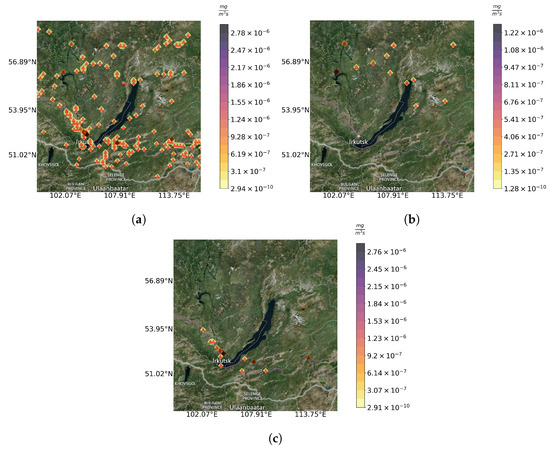
Figure 1.
“True” emission sources : “All” (a), “Invis” (b), “Vis” (c) configurations. Source locations are marked with red triangles.
In the reaction model, we consider chemical species including and . We suppose that only is emitted () with different constant emission rates in the sites presented in Figure 1. Ozone () concentrations are measured () as a snapshot of the concentration field at the final time moment. Measurement noise . The calculations are carried out on a grid of by points in space, corresponding to the geographical domain presented in Figure 1, with points in a time period starting at 2019-07-23 T12:00:00 with a time step of 54 s.
As a target for refinement by means of deep learning, we consider the reconstruction results for and
projection functions.
Figure 2 demonstrates (the result of reconstruction) and its estimate for the “Invis” source configuration with different numbers of projection functions. Analyzing Figure 2a,c, we can see that some of the “true” emission sources are located inside of the reconstructed distributed sources, (producing “excessively smeared point-wise source errors”). We can also see that some of the “true” sources have no explicit corresponding objects in the reconstruction (“false negative errors”) and some of the reconstruction artifacts do not correspond to any “true” sources (“false positive errors”). The ideal refinement algorithm must fix all three types of errors. Another quantitative observation that we have in Figure 2b,d is that the reconstruction estimates have a similar structure in space to the corresponding reconstructions (Figure 2a,c), but the values are different (see the scales).
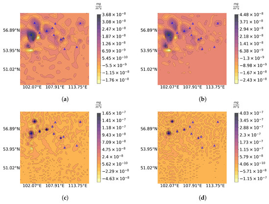
Figure 2.
Reconstruction result (a,c) and its estimate (b,d) for (a,b) and (c,d) in “Invis” configuration. “True” emission sources are marked with blue triangles.
In Figure 3, we present the estimate error with respect to the “true” solution for all the considered numerical experiments:
A significant error is expected since we estimate the nonlinear mapping by affine-type estimation . For example, the differences between Figure 2a,b and Figure 2c,d correspond to the minimal and maximum relative errors, correspondingly.
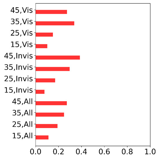
Figure 3.
Reconstruction estimate error with respect to the “true” solution .
In Figure 4, we present the computation times of the inverse problem solutions for the three source configurations and consider the number of the projection functions (13). We carried out the calculations at the Siberian Supercomputer Center on the NKS-1P hybrid cluster by RSC Group, Moscow, Russia using three Intel Xeon Gold 6248R nodes (each has 2 CPU × 24 cores × 2 threads, 3.00 GHz, 384 GB RAM). The total number of cores used is 144. The nodes are connected with Cluster Interconnect Omni-Path 100 Gbps.
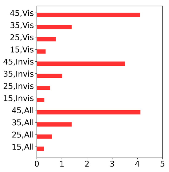
Figure 4.
Emission source reconstruction time in hours by IMDAF.
Analyzing Figure 4, we can see that the computation time is proportional to the number of projection functions; therefore, it makes sense to use deep learning to obtain a solution corresponding to more projection functions from a solution with less functions. This problem resembles a computer tomography inversion problem with incomplete data (limited-angle computer tomography). This problem can be approached using deep learning [38,39,40,41]. For example, in [38], the authors used a U-net-type convolutional neural network and a filtered back-projection computer tomography algorithm to work with incomplete data.
2.5. Deep Learning-Based Refinement of Inverse Modeling Results
The problem of refining the inverse modeling result can be approximated by the problem of inversion of on
To measure the quality of the refinement results, we use two metrics: the interpretation quality
and the complexity of the results . We measure the complexity on as the number of point-wise sources (or positive elements in the discrete setting).
First, let us look at the action of the operator P on point-wise sources. In Figure 5, we present samples of pairs , for and , correspondingly. We note that the approximate reconstruction result corresponding to a smaller number of projection functions contains coarser artifacts compared to the case. Analyzing Figure 5, we note that the problem resembles a deconvolution problem, i.e., the restoration of the original image after the distortion represented by a local convolution operation [42].
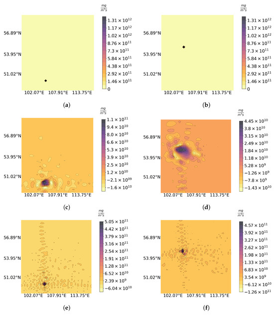
Figure 5.
Training samples (a,b), for (c,d), and for (e,f).
A need for deconvolution arises in various areas—for example, in the compensation of blur caused by the movement of a camera or object at shooting [43], or the correction of optical artifacts in microscopy [44] and astronomy [45]. The case in which the distorting function (convolution operator) is known in advance is “non-blind” deconvolution. In the absence of noise in a distorted image, non-blind deconvolution is achieved by inverting the convolution operator analytically (inverse filtering [42]). For noisy images, this approach leads to unsatisfactory results due to the appearance of significant artifacts caused by the added “deconvolution of noise” [42]. In such cases, the original image is restored using optimization algorithms such as Wiener filtering [46] or Tikhonov regularization [47] (in the frequency domain) or the Luce–Richardson method [48] (in the spatial domain).
Deconvolution for an unknown distorting function (“blind”) is performed by an iterative process, at each step of which the evaluation of the distorting function is refined, and, on its basis, the original image is evaluated using the methods described above [49]. For the evaluation of the distorting functions that one can use, such as machine learning methods, see [50]. In this context, if we consider the linear part of P solely that is the operator (which makes sense as it acts between “increments”), our problem will be close to the problem of non-blind deconvolution in the absence of noise, but with the following reservations:
- the distortion function is spatially variant (i.e., not a local convolution);
- the distortion operator has a non-empty kernel (i.e., inverse filtering is impossible);
- the high-quality restoration of images of the special “several point-wise source” class is of critical importance.
We look for a solution that provides “adequate” interpretation quality and complexity defined by constants and :
In [51], we used deep learning only to obtain a solution of (15). In the present work, we split the problem into two steps: localizing the sources and recovering the emission rates. The reason for this modification is that, provided with the source locations, the estimation of the emission rates is a more straightforward problem. Hence, in the modified algorithm, the first step is performed with the help of deep learning; the second involves solving a quadratic programming problem using the source locations obtained at the first step.
For the localization of sources, we use a neural network operator
where are trainable parameters that have to be estimated with training samples :
where is the training loss function. Due to the complexity of the cost (error) function, we can obtain different optimization results by setting different (random) initial and optimization algorithm parameters in the training procedure.
At this step, we control the complexity of the resulting solution . If is satisfied, is returned as the result of the step; otherwise, we repeat the learning procedure with different initial and optimization algorithm parameters. The localization step can be summarized as an operator that maps to such that .
To recover the emission rates, we solve a quadratic programming problem and describe this step as an operator . Let an element of be
Then, we consider as functions of rates with fixed locations and solve the constrained quadratic optimization problem
In our case, and the cost function in (19) is equivalent to a quadratic polynomial of
where , . Finally,
Considering these two steps sequentially, we obtain an approximation of :
Finally, we check the first requirement (17) on . If , then is considered as an acceptable solution; otherwise, the procedure is repeated from the first step with different parameters in the learning procedure until both requirements (17) and (18) are satisfied. The algorithm is summarized in Figure 6.
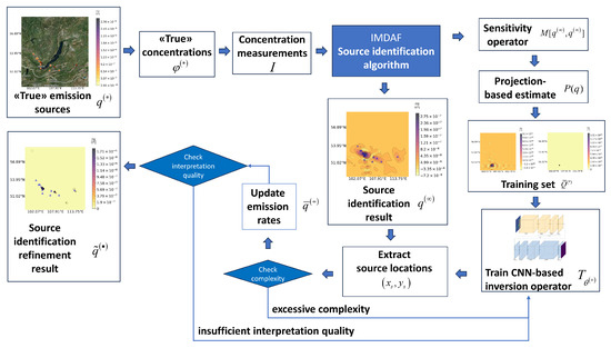
Figure 6.
Refinement algorithm.
2.6. Convolutional Neural Networks
To specify the operator at the localization step of the refinement algorithm, we need to construct a neural network that processes the image, transforming “spots” into “points” and filtering specific artifacts. Convolutional neural networks (CNN) have been reported to successfully solve various image reconstruction [3,52] and image processing tasks, including segmentation [53,54], deblurring [55,56,57], and denoising [58,59]. CNNs can be used in image [60,61] and multivariate time-series (1D image) classification tasks [62,63].
Keeping in mind these works, we tried several CNNs of increasing complexity: CNN3, CNN4, and CNN9, presented in Figure 7 and Table 1. Layers with a larger filter size allow us to identify areas with blurring and to “shrink” the areas to standalone points with a smaller one. The largest network, CNN9, has an encoder–decoder architecture; CNN3 and CNN4 consist of layers of CNN9’s encoder.
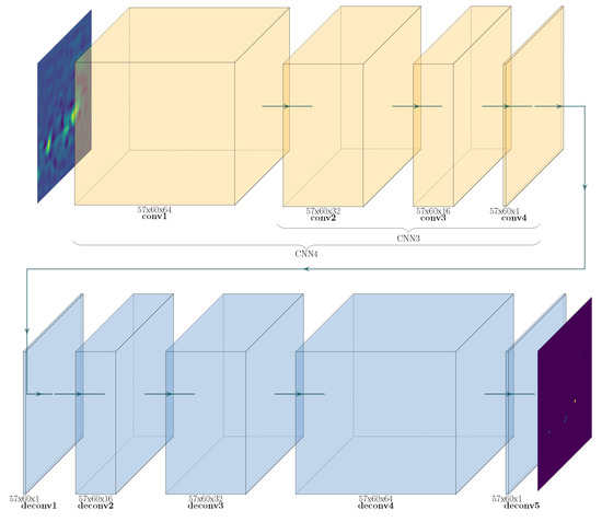
Figure 7.
CNN3, CNN4, and CNN9 architectures.

Table 1.
CNN3, CNN4, and CNN9 layers.
To construct and train the CNN operator , we used standard Tensorflow layers and training (optimization) algorithms. The first layer is an input layer and the last one is an output layer. The following parameters are the same for all the layers: strides = 1, activation = ’relu’, padding = ’same’; ’Adamax’ is the optimizer [64], ’mse’ is the loss and metric function. To reduce the learning rate, when the metric has stopped improving, ReduceLROnPlateau is used with the following parameters: factor = sqrt(0.1), cooldown = 0, patience = 5, min_lr = .
We used a number of training epochs of 10, interpretation quality parameter , complexity threshold . To construct a training set , we use all single point-wise sources localized in different points of the grid domain :
Some examples of elements are presented in Figure 5. We used training and validation samples of and elements, correspondingly, with a batch size of .
3. Results
Figure 8 shows the relative error and the relative complexity of the solutions provided by the above-proposed algorithms. Relative complexity equal to 1 implies that the numbers of point-wise sources in “true” and refined solutions are equal. The error of the CNN-refined projection-based estimation allows us to evaluate the quality of the pure inversion of P on .
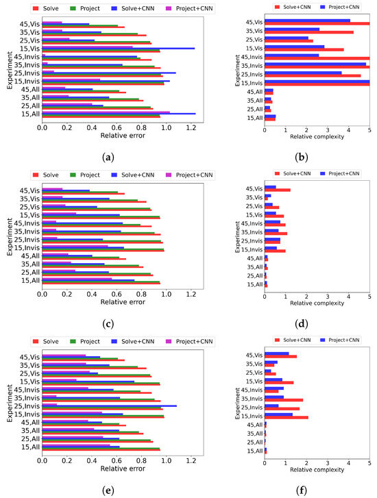
Figure 8.
Relative errors with respect to for CNN3 (a), CNN4 (c), and CNN9 (e); general algorithm’s results (Solve, red), projection-based estimate of result (Project, green), CNN-refined solution (Solve+CNN, blue), and CNN-refined projection-based estimate (Project+CNN, magenta). Relative complexity with respect to for CNN3 (b), CNN4 (d), and CNN9 (f); CNN-refined solution (Solve+CNN, red) and CNN-refined projection-based estimate (Project+CNN, blue).
Figure 9 and Figure 10 show the source identification results obtained with the general algorithm and the results of its refinement with CNN3, CNN4, and CNN9 for different numbers of projection functions and source configurations.
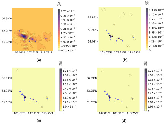
Figure 9.
Source identification result (a) for and results of its refinement by CNN3 (b), CNN4 (c), and CNN9 (d) in “Vis” configuration. “True” sources are marked with blue triangles.
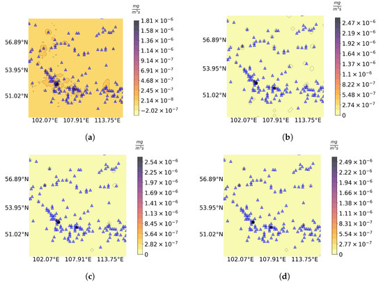
Figure 10.
Source identification result (a) for and results of its refinement by CNN3 (b), CNN4 (c), and CNN9 (d) in “All” configuration. “True” sources are marked with blue triangles.
Analyzing the results in Figure 8, we conclude that, from a quantitative point of view, the best results with respect to relative errors and complexity are obtained with CNN4. In all the cases, the refined solutions have smaller errors compared to the reconstruction results (Figure 8c). CNN3 produced excessively complex solutions (Figure 8b) and, in some cases (with “small” numbers of projection functions and larger artifacts), the error of the refined solution is larger than the error of the rough reconstruction. The performance of CNN9 can be assessed as intermediate between the two. From a qualitative point of view (Figure 9 and Figure 10), the results are similar up to some artifacts.
Since “true” solutions are not known in advance, let us compare the results produced by the above-considered ANN architectures with characteristics that do not take known “true” solutions. Figure 11 demonstrates the interpretation quality (16) (the less, the better) and complexity (the less, the better). Analyzing Figure 11, we conclude that CNN3 almost always provides better solutions with respect to interpretation quality, but significantly concedes in providing simple (or compact) solutions. CNN4 and CNN9 provide similar solutions with respect to complexity, but CNN4 is almost always better than CNN9 in terms of interpretation quality. These results are in accordance with the results shown in Figure 8.
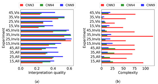
Figure 11.
Interpretation quality (a) and complexity (b) for CNN3 (red), CNN4 (green), and CNN9 (blue).
4. Discussion
Analyzing Figure 8, we conclude that the algorithm provided a significant refinement to the source reconstruction results. We can see that the relative reconstruction error decreases with an increasing projection function number, which reflects the increasing measurement data considered. On the contrary, the refinement results do not show similar monotonicity with respect to the input data and the basic reconstruction quality. This means that the performance of the refinement algorithm depends on the different characteristics of the input data. It may be connected to the quality of the reconstruction estimates, which shows the opposite dependence (Figure 3) on the number of projection functions. This unclear dependence can be considered as a limitation of the algorithm.
The hybrid algorithm performance depends on the properties of the sensitivity operators (e.g., the non-linearity of a sensitivity operator likely impacts the quality of ’s approximations). The sensitivity operators and corresponding right-hand sides of quasi-linear operator equations (6) are defined by the emission source identification problem statement (Section 2.1), which is composed of atmospheric process models, a measurement system, and an unknown function choice. The atmospheric model’s parameters depend on the climatic and geographical conditions of the region under consideration. Therefore, these conditions impact the sensitivity operators in various ways. In this paper, we present an illustration of the approach in realistic conditions for the Baikal region. A further investigation is needed to identify which conditions have significant effects on the sensitivity operator’s properties that are important for the hybrid algorithm’s performance and to estimate its generalizability and reliability for other regions (e.g., in a city air quality inverse modeling scenario, as in [35]).
The key point of the algorithm is the ability to construct a relevant and computationally cheap reconstruction result approximation . In this paper, we provide an example of such an estimate and test its performance in the numerical experiments. Other estimates can also be considered. To reduce the risk of using inaccurate estimates, a strategy including both and its estimate can be developed.
The sensitivity operator that is evaluated in sensitivity operator-based algorithms provides a natural way to generate training samples of any size for various classes of solutions. In this work, we considered a complete set of single point-wise sources as a training set for the localization stage of the refinement algorithm. In future work, we plan to consider training sets containing multiple point-wise sources and piece-wise linear sources. Since the number of such sources is substantially higher than the number of single point-wise sources, which is , some reproducible procedure of constructing an affordable yet representative set of training samples should be developed, e.g., with some type of pseudo-random sequence. Another interesting question is whether it is possible to distinguish the main types of sources (point-wise, linear, and distributed), thus solving a source classification problem.
In contrast to many deep learning applications, where there is a given sample set and ANNs have to correctly process different inputs, in the present paper, we have a direct model that can potentially produce a sample set of any size and a trained ANN has to process only one input . This setting, in some sense, corresponds to the task of constructing a surrogate of a complicated model. In these terms, we construct a surrogate of the inverse on using its approximation P, deep learning, and quadratic programming.
Using standard deep learning terminology, we can formally consider as a testing set consisting of a single element. In real applications, is unknown, but we can potentially use multi-point sources in the vicinity of to construct a larger testing set. This may be the subject of future research. We can also consider the whole set of the above-presented 12 numerical experiments as a testing set for a hybrid algorithm.
The risk of overfitting in the proposed framework is reduced by the following hybrid algorithm’s features. In our setting, the training samples are significantly different from the target input : each training sample corresponds to a single point-wise source, while the target sample contains multiple point-wise sources. Furthermore, according to the algorithm (Figure 6), in the case of unsatisfactory results (by criteria (17) and (18)) for a target input, we can abandon the refinement result and look for another. Thanks to the criteria, instead of an ANN, we can potentially use a random generator or any appropriate metaheuristic algorithm, but the ANN is supposed to produce more targeted results, thus decreasing the number of attempts. In our case, typical overfitting appears as a trained ANN producing a zero output for a target input , which can be identified with (17).
Another important question is the choice of the training loss metric. We used the standard mean squared error (mse) since it is fast enough and works with both Q (distributed) and (point-wise) functions in discrete settings. A limitation of mse for this setting is that it does not measure the distance between point-wise sources. The distance metrics of Hausdorff, Chamfer, or Wassershtein appear more suitable, but additional work is needed to obtain their sufficiently fast implementation for the comparison of distributed and point-wise sources.
To update the emission rates at the second step of the refinement algorithm, we use the estimate . To obtain a better estimate of the emission rates, it is possible to use (6) or consider an emission rate identification problem with fixed source locations. Additionally, in this paper, we consider an algorithm with only one iteration of the refinement procedure. Refinement can be done iteratively, i.e., the procedure can be repeated for the residual:
Interpretation quality (the less, the better) is quantified by (16), involving the operator P. A more rigorous evaluation of the interpretation quality can be carried out by using the operator instead of P in (16), which uses the solution of the inverse problem and therefore is more time-consuming (Figure 4). Evaluating the direct problem operator and comparing the corresponding values to measurement data I directly would be less time-consuming and more appropriate in the context of a source identification problem.
The upper boundary of admissible interpretation quality in (17) was experimentally chosen to be small enough to avoid overfitted ANN results (e.g., ) and large enough to reduce the number of iterations due to the violation of (17). The parameter of the second criterion (18) was chosen to avoid “smeared” solutions (e.g., if , then , and fits the first criterion (17), but ). A more automated procedure for the selection of criteria parameters can be considered as a direction of further research.
In this paper, we evaluated the refinement of a solution obtained by the basic source identification algorithm. In order to evaluate the performance of the whole hybrid algorithm in the context of source identification, it should be compared to specialized point-wise source identification algorithms (e.g., [11,12,13,14,15,16]). This can be considered as a future research direction.
The question of choosing the correct ANN architecture is also an important one. We present a comparison of the results produced by the above-considered CNN architectures based on relative errors, interpretation quality, and solution complexity, but further investigation is also needed in this direction.
In this paper, we consider image-type measurements, when a spatial domain is equivalently visible by a measurement system. In the case of localized measurements, spatially different illumination becomes an important issue [31,32,33]. In this case, a source reconstruction algorithm tends to place maxima of the reconstructed sources in measurement points. To fix this distortion, the authors of [31,32,33] introduced a re-normalization concept to preserve the locations of the maxima. A refinement algorithm for localized measurements will be the subject of future research. Another important question is measurement noise. Machine learning denoising may be applied in this direction. In this case, it may be implemented as a pre-possessing algorithm in the space of the measurement results.
5. Conclusions
In this paper, we numerically tested a source identification algorithm that combines a general-type emission source identification stage and a post-processing refinement stage. Emission source identification by measurement data is carried out with a sensitivity operator-based algorithm. At the post-processing stage, the general-type emission source identified at the first stage is transformed into a source consisting of multiple point-wise sources. The second stage consists of two steps: point-wise source localization and emission rate estimation. The first step is carried out using deep learning with convolutional neural networks. Training samples are generated using the sensitivity operator obtained at the first step. The algorithm was tested in regional remote sensing emission source identification scenarios for the Lake Baikal region and was able to refine the emission source reconstruction results.
Hybrid approaches combining machine learning with traditional inverse problem solution methods emerge as a promising direction for the further development of inverse modeling algorithms. Moreover, aggregates used in traditional inverse problem solution algorithms can be successfully applied within machine learning frameworks to produce hybrid algorithms.
Author Contributions
Conceptualization, A.P.; methodology, A.P. and M.E.; software, A.P., M.E. and E.T.; validation, A.P., M.E. and E.R.; formal analysis, E.R.; investigation, A.P. and M.E.; resources, A.P.; data curation, A.P.; writing—original draft preparation, A.P.; writing—review and editing, A.P., E.R. and V.S.; visualization, A.P., E.R. and V.S.; supervision, A.P.; project administration, A.P.; funding acquisition, A.P. All authors have read and agreed to the published version of the manuscript.
Funding
The work was supported by grant 075-15-2020-787 in the form of a subsidy for a Major Scientific Project from the Ministry of Science and Higher Education of Russia (project “Fundamentals, methods and technologies for digital monitoring and forecasting of the environmental situation on the Baikal Natural Territory”).
Data Availability Statement
Data are available on request.
Conflicts of Interest
The authors declare no conflicts of interest. The funders had no role in the design of the study; in the collection, analyses, or interpretation of data; in the writing of the manuscript, or in the decision to publish the results.
References
- Arridge, S.; Maass, P.; Oktem, O.; Schonlieb, C.B. Solving inverse problems using data-driven models. Acta Numer. 2019, 28, 1–174. [Google Scholar] [CrossRef]
- Bonavita, M.; Laloyaux, P. Machine Learning for Model Error Inference and Correction. J. Adv. Model. Earth Syst. 2020, 12, e2020MS002232. [Google Scholar] [CrossRef]
- Yedder, H.B.; Cardoen, B.; Hamarneh, G. Deep learning for biomedical image reconstruction: A survey. Artif. Intell. Rev. 2020, 54, 215–251. [Google Scholar] [CrossRef]
- Amjad, J.; Lyu, Z.; Rodrigues, M.R.D. Deep Learning Model-Aware Regulatization With Applications to Inverse Problems. IEEE Trans. Signal Process. 2021, 69, 6371–6385. [Google Scholar] [CrossRef]
- Kamyab, S.; Azimifar, Z.; Sabzi, R.; Fieguth, P. Deep learning methods for inverse problems. PeerJ Comput. Sci. 2022, 8, e951. [Google Scholar] [CrossRef] [PubMed]
- Markakis, K.; Valari, M.; Perrussel, O.; Sanchez, O.; Honore, C. Climate-forced air-quality modeling at the urban scale: Sensitivity to model resolution, emissions and meteorology. Atmos. Chem. Phys. 2015, 15, 7703–7723. [Google Scholar] [CrossRef]
- Holnicki, P.; Nahorski, Z. Emission Data Uncertainty in Urban Air Quality Modeling—Case Study. Environ. Model. Assess. 2015, 20, 583–597. [Google Scholar] [CrossRef]
- Daubechies, I.; Defrise, M.; Mol, C.D. An iterative thresholding algorithm for linear inverse problems with a sparsity constraint. Commun. Pure Appl. Math. 2004, 57, 1413–1457. [Google Scholar] [CrossRef]
- Teschke, G.; Ramlau, R. An iterative algorithm for nonlinear inverse problems with joint sparsity constraints in vector-valued regimes and an application to color image inpainting. Inverse Probl. 2007, 23, 1851–1870. [Google Scholar] [CrossRef]
- Jin, B.; Maass, P. Sparsity regularization for parameter identification problems. Inverse Probl. 2012, 28, 123001. [Google Scholar] [CrossRef]
- Badia, A.E.; Ha-Duong, T.; Hamdi, A. Identification of a point source in a linear advection–dispersion–reaction equation: Application to a pollution source problem. Inverse Probl. 2005, 21, 1121–1136. [Google Scholar] [CrossRef]
- Badia, A.E.; Hamdi, A. Inverse source problem in an advection–dispersion–reaction system: Application to water pollution. Inverse Probl. 2007, 23, 2103–2120. [Google Scholar] [CrossRef]
- Mamonov, A.V.; Tsai, Y.H.R. Point source identification in nonlinear advection-diffusion-reaction systems. Inverse Probl. 2013, 29, 035009. [Google Scholar] [CrossRef]
- Desyatkov, B.M.; Lapteva, N.A.; Shabanov, A.N. Mathematical method for searching unknown point sources of gas and aerosol in the atmosphere. Atmos. Ocean. Opt. 2015, 28, 518–521. [Google Scholar] [CrossRef]
- Ren, K.; Zhong, Y. Imaging point sources in heterogeneous environments. Inverse Probl. 2019, 35, 125003. [Google Scholar] [CrossRef]
- Pyatkov, S.G.; Rotko, V.V. Inverse Problems with Pointwise Overdetermination for some Quasilinear Parabolic Systems. Sib. Adv. Math. 2020, 30, 124–142. [Google Scholar] [CrossRef]
- Liao, Q.; Zhu, M.; Wu, L.; Pan, X.; Tang, X.; Wang, Z. Deep Learning for Air Quality Forecasts: A Review. Curr. Pollut. Rep. 2020, 6, 399–409. [Google Scholar] [CrossRef]
- Liu, X.; Lu, D.; Zhang, A.; Liu, Q.; Jiang, G. Data-Driven Machine Learning in Environmental Pollution: Gains and Problems. Environ. Sci. Technol. 2022, 56, 2124–2133. [Google Scholar] [CrossRef]
- Xu, J.; Du, W.; Xu, Q.; Dong, J.; Wang, B. Federated learning based atmospheric source term estimation in urban environments. Comput. Chem. Eng. 2021, 155, 107505. [Google Scholar] [CrossRef]
- Pan, Z.; Lu, W.; Fan, Y.; Li, J. Identification of groundwater contamination sources and hydraulic parameters based on bayesian regularization deep neural network. Environ. Sci. Pollut. Res. 2021, 28, 16867–16879. [Google Scholar] [CrossRef]
- Wan, H.; Xu, R.; Zhang, M.; Cai, Y.; Li, J.; Shen, X. A novel model for water quality prediction caused by non-point sources pollution based on deep learning and feature extraction methods. J. Hydrol. 2022, 612, 128081. [Google Scholar] [CrossRef]
- He, T.L.; Jones, D.B.A.; Miyazaki, K.; Bowman, K.W.; Jiang, Z.; Chen, X.; Li, R.; Zhang, Y.; Li, K. Inverse modelling of Chinese NOx emissions using deep learning: Integrating in situ observations with a satellite-based chemical reanalysis. Atmos. Chem. Phys. 2022, 22, 14059–14074. [Google Scholar] [CrossRef]
- Zhou, Y.; An, Y.; Huang, W.; Chen, C.; You, R. A combined deep learning and physical modelling method for estimating air pollutants’ source location and emission profile in street canyons. Build. Environ. 2022, 219, 109246. [Google Scholar] [CrossRef]
- Lang, Z.; Wang, B.; Wang, Y.; Cao, C.; Peng, X.; Du, W.; Qian, F. A Novel Multi-Sensor Data-Driven Approach to Source Term Estimation of Hazardous Gas Leakages in the Chemical Industry. Processes 2022, 10, 1633. [Google Scholar] [CrossRef]
- Luo, C.; Lu, W.; Pan, Z.; Bai, Y.; Dong, G. Simultaneous identification of groundwater pollution source and important hydrogeological parameters considering the noise uncertainty of observational data. Environ. Sci. Pollut. Res. 2023, 30, 84267–84282. [Google Scholar] [CrossRef] [PubMed]
- Reich, S.; Gomez, D.; Dawidowski, L. Artificial neural network for the identification of unknown air pollution sources. Atmos. Environ. 1999, 33, 3045–3052. [Google Scholar] [CrossRef]
- Zhang, T.H.; You, X.Y. Applying neural networks to solve the inverse problem of indoor environment. Indoor Built Environ. 2013, 23, 1187–1195. [Google Scholar] [CrossRef]
- Penenko, A. Convergence analysis of the adjoint ensemble method in inverse source problems for advection-diffusion-reaction models with image-type measurements. Inverse Probl. Imaging 2020, 14, 757–782. [Google Scholar] [CrossRef]
- Penenko, A.; Penenko, V.; Tsvetova, E.; Gochakov, A.; Pyanova, E.; Konopleva, V. Sensitivity Operator Framework for Analyzing Heterogeneous Air Quality Monitoring Systems. Atmosphere 2021, 12, 1697. [Google Scholar] [CrossRef]
- Marchuk, G.I. Formulation of some converse problems. Sov. Math. Dokl. 1964, 5, 675–678. [Google Scholar]
- Issartel, J.P. Rebuilding sources of linear tracers after atmospheric concentration measurements. Atmos. Chem. Phys. 2003, 3, 2111–2125. [Google Scholar] [CrossRef]
- Issartel, J.P. Emergence of a tracer source from air concentration measurements, a new strategy for linear assimilation. Atmos. Chem. Phys. 2005, 5, 249–273. [Google Scholar] [CrossRef]
- Turbelin, G.; Singh, S.; Issartel, J.P.; Busch, X.; Kumar, P. Computation of Optimal Weights for Solving the Atmospheric Source Term Estimation Problem. J. Atmos. Ocean. Technol. 2019, 36, 1053–1061. [Google Scholar] [CrossRef]
- Penenko, A.; Penenko, V.; Tsvetova, E.; Mukatova, Z. Consistent Discrete-Analytical Schemes for the Solution of the Inverse Source Problems for Atmospheric Chemistry Models with Image-Type Measurement Data. In Finite Difference Methods. Theory and Applications; Lecture Notes in Computer Science; Springer: Berlin/Heidelberg, Germany, 2019; pp. 378–386. [Google Scholar] [CrossRef]
- Penenko, V.V.; Penenko, A.V.; Tsvetova, E.A.; Gochakov, A.V. Methods for Studying the Sensitivity of Air Quality Models and Inverse Problems of Geophysical Hydrothermodynamics. J. Appl. Mech. Tech. Phys. 2019, 60, 392–399. [Google Scholar] [CrossRef]
- Menke, W. Geophysical Data Analysis Discrete Inverse Theory; Academic Press: Cambridge, MA, USA, 2012. [Google Scholar]
- Cheverda, V.A.; Kostin, V.I. R-pseudoinverses for compact operators in Hilbert spaces: Existence and stability. J. Inverse Ill-Posed Probl. 1995, 3, 131–148. [Google Scholar] [CrossRef]
- Dong, J.; Fu, J.; He, Z. A deep learning reconstruction framework for X-ray computed tomography with incomplete data. PLoS ONE 2019, 14, e0224426. [Google Scholar] [CrossRef] [PubMed]
- Hu, D.; Zhang, Y.; Liu, J.; Du, C.; Zhang, J.; Luo, S.; Quan, G.; Liu, Q.; Chen, Y.; Luo, L. SPECIAL: Single-Shot Projection Error Correction Integrated Adversarial Learning for Limited-Angle CT. IEEE Trans. Comput. Imaging 2021, 7, 734–746. [Google Scholar] [CrossRef]
- Hu, D.; Zhang, Y.; Liu, J.; Luo, S.; Chen, Y. DIOR: Deep Iterative Optimization-Based Residual-Learning for Limited-Angle CT Reconstruction. IEEE Trans. Med. Imaging 2022, 41, 1778–1790. [Google Scholar] [CrossRef]
- Hu, D.; Zhang, Y.; Li, W.; Zhang, W.; Reddy, K.; Ding, Q.; Zhang, X.; Chen, Y.; Gao, H. SEA-Net: Structure-Enhanced Attention Network for Limited-Angle CBCT Reconstruction of Clinical Projection Data. IEEE Trans. Instrum. Meas. 2023, 72, 4507613. [Google Scholar] [CrossRef]
- Gonzalez, R.; Woods, R. Digital Image Processing; Pearson: London, UK, 2018. [Google Scholar]
- Huihui, Y.; Daoliang, L.; Yingyi, C. A state-of-the-art review of image motion deblurring techniques in precision agriculture. Heliyon 2023, 9, e17332. [Google Scholar] [CrossRef]
- Goodwin, P.C. Chapter 10—Quantitative deconvolution microscopy. In Quantitative Imaging in Cell Biology; Waters, J.C., Wittman, T., Eds.; Academic Press: Cambridge, MA, USA, 2014; Volume 123, pp. 177–192. [Google Scholar] [CrossRef]
- Starck, J.L.; Pantin, E.; Murtagh, F. Deconvolution in Astronomy: A Review. Publ. Astron. Soc. Pac. 2002, 114, 1051–1069. [Google Scholar] [CrossRef]
- Wiener, N. Extrapolation, Interpolation, and Smoothing of Stationary Time Series: With Engineering Applications; Technology Press Books in Science and Engineering; MIT Press: Cambridge, MA, USA, 1949. [Google Scholar]
- Tikhonov, A.; Leonov, A.; Yagola, A. Nonlinear Ill-Posed Problems; Applied mathematics and mathematical computation; Chapman & Hall: Boca Raton, FL, USA, 1998. [Google Scholar]
- Lucy, L.B. An iterative technique for the rectification of observed distributions. Astron. J. 1974, 79, 745–754. [Google Scholar] [CrossRef]
- Levin, A.; Weiss, Y.; Durand, F.; Freeman, W.T. Understanding and evaluating blind deconvolution algorithms. In Proceedings of the 2009 IEEE Conference on Computer Vision and Pattern Recognition, Miami, FL, USA, 20–25 June 2009; pp. 1964–1971. [Google Scholar] [CrossRef]
- Shajkofci, A.; Liebling, M. Spatially-Variant CNN-Based Point Spread Function Estimation for Blind Deconvolution and Depth Estimation in Optical Microscopy. IEEE Trans. Image Process. 2020, 29, 5848–5861. [Google Scholar] [CrossRef] [PubMed]
- Penenko, A.; Emelyanov, M.; Tsybenova, E. Deep Learning-based Refinement of the Emission Source Identification Results. In Proceedings of the 2023 19th International Asian School-Seminar on Optimization Problems of Complex Systems (OPCS), Novosibirsk, Russia, 14–22 August 2023. [Google Scholar] [CrossRef]
- Jin, K.H.; McCann, M.T.; Froustey, E.; Unser, M. Deep Convolutional Neural Network for Inverse Problems in Imaging. IEEE Trans. Image Process. 2017, 26, 4509–4522. [Google Scholar] [CrossRef] [PubMed]
- Shelhamer, E.; Long, J.; Darrell, T. Fully Convolutional Networks for Semantic Segmentation. IEEE Trans. Pattern Anal. Mach. Intell. 2017, 39, 640–651. [Google Scholar] [CrossRef] [PubMed]
- Ulku, I.; Akagündüz, E. A Survey on Deep Learning-based Architectures for Semantic Segmentation on 2D Images. Appl. Artif. Intell. 2022, 36, 2032924. [Google Scholar] [CrossRef]
- Kupyn, O.; Budzan, V.; Mykhailych, M.; Mishkin, D.; Matas, J. DeblurGAN: Blind Motion Deblurring Using Conditional Adversarial Networks. In Proceedings of the 2018 IEEE/CVF Conference on Computer Vision and Pattern Recognition, Salt Lake City, UT, USA, 18–23 June 2018. [Google Scholar] [CrossRef]
- Koh, J.; Lee, J.; Yoon, S. Single-image deblurring with neural networks: A comparative survey. Comput. Vis. Image Underst. 2021, 203, 103134. [Google Scholar] [CrossRef]
- Zhang, K.; Ren, W.; Luo, W.; Lai, W.S.; Stenger, B.; Yang, M.H.; Li, H. Deep Image Deblurring: A Survey. Int. J. Comput. Vis. 2022, 130, 2103–2130. [Google Scholar] [CrossRef]
- Zhang, K.; Zuo, W.; Chen, Y.; Meng, D.; Zhang, L. Beyond a Gaussian Denoiser: Residual Learning of Deep CNN for Image Denoising. IEEE Trans. Image Process. 2017, 26, 3142–3155. [Google Scholar] [CrossRef]
- Zheng, M.; Zhi, K.; Zeng, J.; Tian, C.; You, L. A Hybrid CNN for Image Denoising. J. Artif. Intell. Technol. 2022, 2, 93–99. [Google Scholar] [CrossRef]
- Rawat, W.; Wang, Z. Deep Convolutional Neural Networks for Image Classification: A Comprehensive Review. Neural Comput. 2017, 29, 2352–2449. [Google Scholar] [CrossRef]
- Kumar, N.; Kaur, N.; Gupta, D. Major Convolutional Neural Networks in Image Classification: A Survey. In Lecture Notes in Networks and Systems; Springer: Singapore, 2020; pp. 243–258. [Google Scholar] [CrossRef]
- Koh, B.H.D.; Lim, C.L.P.; Rahimi, H.; Woo, W.L.; Gao, B. Deep Temporal Convolution Network for Time Series Classification. Sensors 2021, 21, 603. [Google Scholar] [CrossRef]
- Lee, X.Y.; Kumar, A.; Vidyaratne, L.; Rao, A.R.; Farahat, A.; Gupta, C. An ensemble of convolution-based methods for fault detection using vibration signals. In Proceedings of the 2023 IEEE International Conference on Prognostics and Health Management (ICPHM), Montreal, QC, Canada, 5–7 June 2023. [Google Scholar] [CrossRef]
- Kingma, D.P.; Ba, J. Adam: A Method for Stochastic Optimization. arXiv 2014, arXiv:1412.6980. [Google Scholar]
Disclaimer/Publisher’s Note: The statements, opinions and data contained in all publications are solely those of the individual author(s) and contributor(s) and not of MDPI and/or the editor(s). MDPI and/or the editor(s) disclaim responsibility for any injury to people or property resulting from any ideas, methods, instructions or products referred to in the content. |
© 2023 by the authors. Licensee MDPI, Basel, Switzerland. This article is an open access article distributed under the terms and conditions of the Creative Commons Attribution (CC BY) license (https://creativecommons.org/licenses/by/4.0/).