Article

The Confluent Hypergeometric Beta Distribution

1
Department of Mathematics, University of Manchester, Manchester M13 9PL, UK
2
Department of Mathematics, Howard University, Washington, DC 20059, USA
*
Author to whom correspondence should be addressed.
Mathematics 2023, 11(9), 2169; https://doi.org/10.3390/math11092169
Submission received: 9 April 2023 / Revised: 28 April 2023 / Accepted: 2 May 2023 / Published: 5 May 2023

Abstract

:
The confluent hypergeometric beta distribution due to Gordy has been known since the 1990s, but not much of is known in terms of its mathematical properties. In this paper, we provide a comprehensive treatment of mathematical properties of the confluent hypergeometric beta distribution. We derive shape properties of its probability density function and expressions for its cumulative distribution function, hazard rate function, reversed hazard rate function, moment generating function, characteristic function, moments, conditional moments, entropies, and stochastic orderings. We also derive procedures for maximum likelihood estimation and assess their finite sample performance. Most of the derived properties are new. Finally, we illustrate two real data applications of the confluent hypergeometric beta distribution.

1. Introduction

Ref. [1] introduced the confluent hypergeometric beta distribution given by the probability density function
f X ( x ) = K x a 1 ( 1 x ) b 1 exp ( c x )
for 0 < x < 1 , a > 0 , b > 0 and < c < , where
1 K = B ( a , b ) 1 F 1 a ;   a + b ;   c ,
where B ( a , b ) and 1 F 1 a , b ;   c ;   x are the beta and confluent hypergeometric functions defined by
B ( a , b ) = 0 1 t a 1 ( 1 t ) b 1 d t
and
1 F 1 a ;   b ;   x = k = 0 ( a ) k ( b ) k x k k ! ,
respectively, where ( a ) k = a ( a + 1 ) ( a + k 1 ) denotes the ascending factorial. The beta function can also be expressed as B ( a , b ) = Γ ( a ) Γ ( b ) / Γ ( a + b ) , where Γ ( a ) denotes the gamma function defined by
Γ ( a ) = 0 t a 1 exp ( t ) d t .
The standard beta distribution is the particular case of (1) for c = 0 . If X is a confluent hypergeometric beta random variable with parameters ( a , b , c ) , then 1 X is also a confluent hypergeometric beta random variable with parameters b , a , c . Hence, X is symmetric if and only if c = 0 .
There have been only a few papers studying the confluent hypergeometric beta distribution. Ref. [2] proposed an exponentiated version of (1). Refs. [3,4] used (1) in Bayesian estimation. Ref. [5] proposed a six-parameter generalization of (1).
The aim of this paper is to provide a comprehensive account of mathematical properties of (1). The properties derived include the shape properties of the probability density function (Section 2), cumulative distribution function (Section 3), hazard rate and reversed hazard rate functions (Section 4), moment generating and characteristic functions (Section 5), moments (Section 6), conditional moments (Section 7), entropies (Section 8), and stochastic orderings (Section 9). We also derive procedures for maximum likelihood estimation (Section 10) and assess their finite sample performance (Section 11). Two real data applications of the confluent hypergeometric beta distribution are illustrated in Section 12. Some conclusions and future work are noted in Section 13.
In addition to the special functions stated, the calculations of this paper involve the degenerate hypergeometric series of two variables defined by
Φ 1 a , b , c , x , y = m = 0 n = 0 ( a ) m + n ( b ) n x m y n ( c ) m + n m ! n ! .
The properties of the special functions can be found in [6,7].

2. Shape

The critical points of f X ( x ) are the roots of
d log f X ( x ) d x = a 1 x b 1 1 x c = 0
or equivalently the roots of
A + B x + C x 2 = 0 ,
where A = a 1 , B = 2 a b c and C = c . Let δ 1 = B B 2 4 A C / ( 2 C ) and δ 2 = B + B 2 4 A C / ( 2 C ) denote the roots of (2). If c = 0 , then the only root is a 1 a + b 2 .
The following shapes are possible for the probability density function:
(a)
if 0 δ 1 < δ 2 1 ,
a 1 δ 1 2 b 1 1 δ 1 2 < 0
and
a 1 δ 2 2 b 1 1 δ 2 2 < 0
then f ( x ) has one mode followed by another mode.
(b)
if 0 δ 1 < δ 2 1 ,
a 1 δ 1 2 b 1 1 δ 1 2 > 0
and
a 1 δ 2 2 b 1 1 δ 2 2 > 0
then f ( x ) has one antimode followed by another antimode.
(c)
if 0 δ 1 < δ 2 1 ,
a 1 δ 1 2 b 1 1 δ 1 2 < 0
and
a 1 δ 2 2 b 1 1 δ 2 2 > 0
then f ( x ) has one mode followed by an antimode.
(d)
if 0 δ 1 < δ 2 1 ,
a 1 δ 1 2 b 1 1 δ 1 2 > 0
and
a 1 δ 2 2 b 1 1 δ 2 2 < 0
then f ( x ) has an antimode followed by a mode.
(e)
if δ 1 < 0 δ 2 1 and
a 1 δ 2 2 b 1 1 δ 2 2 < 0
then f ( x ) has a single mode.
(f)
if δ 1 < 0 δ 2 1 and
a 1 δ 2 2 b 1 1 δ 2 2 > 0
then f ( x ) has a single antimode.
(g)
if 0 δ 1 1 < δ 2 and
a 1 δ 1 2 b 1 1 δ 1 2 < 0
then f ( x ) has a single mode.
(h)
if 0 δ 1 1 < δ 2 and
a 1 δ 1 2 b 1 1 δ 1 2 > 0
then f ( x ) has a single antimode.
(i)
if
a 1 x b 1 1 x < c
for all 0 x 1 then f ( x ) is monotonically decreasing.
(j)
if
a 1 x b 1 1 x > c
for all 0 x 1 then f ( x ) is monotonically increasing.
Possible shapes of f ( x ) are illustrated in Figure 1. Many of the shapes illustrated cannot be exhibited by a standard beta distribution.

3. Cumulative Distribution Function

By equation (2.3.8.1) in volume 1 of [7], the cumulative distribution function of X is
F X ( x ) = K 0 x y a 1 ( 1 y ) b 1 exp ( c y ) d y = K x a a Φ 1 a , 1 b , a + 1 ;   x , c x .
The quantile function defined by F X Q ( p ) = p is the root of
K Q ( p ) a a Φ 1 a , 1 b , a + 1 ;   Q ( p ) , c Q ( p ) = p .
In particular, the median of X, Q ( 1 / 2 ) , is the root of K Q ( 1 / 2 ) a a Φ 1 ( a , 1 b , a + 1 ;   Q ( 1 / 2 ) , c Q ( 1 / 2 ) ) = 1 / 2 .

4. Hazard Rate Functions

It is immediate from (1) and Section 3 that the hazard rate function of X is
h X ( x ) = f X ( x ) 1 F X ( x ) = a K x a 1 ( 1 x ) b 1 exp ( c x ) a K x a Φ 1 a , 1 b , a + 1 ;   x , c x .
It is also immediate that the reversed hazard rate function of X is
r X ( x ) = f X ( x ) F X ( x ) = a ( 1 x ) b 1 exp ( c x ) x Φ 1 a , 1 b , a + 1 ;   x , c x .

5. Moment-Generating and Characteristic Functions

The moment-generating function of X is
M X ( t ) = E exp ( t X ) = K 0 1 x a 1 ( 1 x ) b 1 exp ( c t ) x d x = 1 F 1 a ;   a + b ;   c 1 F 1 a ;   a + b ;   t c .
The corresponding characteristic function is
ϕ X ( t ) = E exp ( i t X ) = 1 F 1 a ;   a + b ;   c 1 F 1 a ;   a + b ;   i t c ,
where i = 1 .

6. Moments

The nth moment of X is
E X n = K 0 1 x n + a 1 ( 1 x ) b 1 exp ( c x ) d x = B ( n + a , b ) 1 F 1 n + a ;   n + a + b ;   c B ( a , b ) 1 F 1 a ;   a + b ;   c .
In particular, the first four moments are
E X = a a + b 1 F 1 1 + a ;   1 + a + b ;   c 1 F 1 a ;   a + b ;   c ,
E X 2 = a ( a + 1 ) ( a + b ) ( a + b + 1 ) 1 F 1 2 + a ;   2 + a + b ;   c 1 F 1 a ;   a + b ;   c ,
E X 3 = a ( a + 1 ) ( a + 2 ) ( a + b ) ( a + b + 1 ) ( a + b + 2 ) 1 F 1 3 + a ;   3 + a + b ;   c 1 F 1 a ;   a + b ;   c
and
E X 4 = a ( a + 1 ) ( a + 2 ) ( a + 3 ) ( a + b ) ( a + b + 1 ) ( a + b + 2 ) ( a + b + 3 ) 1 F 1 4 + a ;   4 + a + b ;   c 1 F 1 a ;   a + b ;   c .
The harmonic means of X are
E 1 X 1 = K 0 1 x a 2 ( 1 x ) b 1 exp ( c x ) d x 1 = B ( a , b ) B ( a 1 , b ) 1 F 1 a ;   a + b ;   c 1 F 1 a 1 ;   a + b 1 ;   c = a a + b 1 1 F 1 a ;   a + b ;   c 1 F 1 a 1 ;   a + b 1 ;   c
and
E 1 1 X 1 = K 0 1 x a 1 ( 1 x ) b 2 exp ( c x ) d x 1 = B ( a , b ) B ( a , b 1 ) 1 F 1 a ;   a + b ;   c 1 F 1 a ;   a + b 1 ;   c = b a + b 1 1 F 1 a ;   a + b ;   c 1 F 1 a ;   a + b 1 ;   c .
Further,
Var 1 X = K 0 1 x a 3 ( 1 x ) b 1 exp ( c x ) d x ( a + b 1 ) 2 a 2 1 F 1 a 1 ;   a + b 1 ;   c 1 F 1 a ;   a + b ;   c 2 = B ( a 2 , b ) B ( a , b ) 1 F 1 a 2 ;   a + b 2 ;   c 1 F 1 a ;   a + b ;   c ( a + b 1 ) 2 a 2 1 F 1 a 1 ;   a + b 1 ;   c 1 F 1 a ;   a + b ;   c 2 = ( a + b 1 ) ( a + b 2 ) a ( a 1 ) 1 F 1 a 2 ;   a + b 2 ;   c 1 F 1 a ;   a + b ;   c ( a + b 1 ) 2 a 2 1 F 1 a 1 ;   a + b 1 ;   c 1 F 1 a ;   a + b ;   c 2
and
Var 1 1 X = K 0 1 x a 1 ( 1 x ) b 3 exp ( c x ) d x ( a + b 1 ) 2 b 2 1 F 1 a ;   a + b 1 ;   c 1 F 1 a ;   a + b ;   c 2 = B ( a , b 2 ) B ( a , b ) 1 F 1 a ;   a + b 2 ;   c 1 F 1 a ;   a + b ;   c ( a + b 1 ) 2 b 2 1 F 1 a ;   a + b 1 ;   c 1 F 1 a ;   a + b ;   c 2 = ( a + b 1 ) ( a + b 2 ) b ( b 1 ) 1 F 1 a ;   a + b 2 ;   c 1 F 1 a ;   a + b ;   c ( a + b 1 ) 2 b 2 1 F 1 a ;   a + b 1 ;   c 1 F 1 a ;   a + b ;   c 2 .
The expressions for the nth moment were previously given in [4].

7. Conditional Moments

By equation (2.3.8.1) in volume 1 of [7], the nth conditional moment of X is
E X n X > x = 1 1 F X ( x ) E X n K 0 x y n + a 1 ( 1 y ) b 1 exp ( c y ) d y = 1 1 F X ( x ) [ B ( n + a , b ) 1 F 1 n + a ;   n + a + b ;   c B ( a , b ) 1 F 1 a ;   a + b ;   c K x a + n a + n Φ 1 a + n , 1 b , a + n + 1 ;   x , c x ] .
In particular, the first four conditional moments are
E X X > x = 1 1 F X ( x ) [ a a + b 1 F 1 1 + a ;   1 + a + b ;   c 1 F 1 a ;   a + b ;   c K x a + 1 a + 1 Φ 1 a + 1 , 1 b , a + 2 ;   x , c x ] ,
E X 2 X > x = 1 1 F X ( x ) [ a ( a + 1 ) ( a + b ) ( a + b + 1 ) 1 F 1 2 + a ;   2 + a + b ;   c 1 F 1 a ;   a + b ;   c K x a + 2 a + 2 Φ 1 a + 2 , 1 b , a + 3 ;   x , c x ] ,
E X 3 X > x = 1 1 F X ( x ) [ a ( a + 1 ) ( a + 2 ) ( a + b ) ( a + b + 1 ) ( a + b + 2 ) 1 F 1 3 + a ;   3 + a + b ;   c 1 F 1 a ;   a + b ;   c K x a + 3 a + 3 Φ 1 a + 3 , 1 b , a + 4 ;   x , c x ]
and
E X 4 X > x = 1 1 F X ( x ) [ a ( a + 1 ) ( a + 2 ) ( a + 3 ) ( a + b ) ( a + b + 1 ) ( a + b + 2 ) ( a + b + 3 ) 1 F 1 4 + a ;   4 + a + b ;   c 1 F 1 a ;   a + b ;   c K x a + 4 a + 4 Φ 1 a + 4 , 1 b , a + 5 ;   x , c x ] .
Note that E ( X X > x ) x and E X 2 X > x E ( X X > x ) 2 are the mean residual life and variance residual functions, respectively.

8. Entropies

The three most popular entropies are the geometric mean [8,9], Shannon entropy [10,11], and Rényi entropy [12], defined by
G M ( X ) = exp log x f X ( x ) d x ,
S ( X ) = log f X ( x ) f X ( x ) d x
and
R ( X ) = 1 1 α log f X ( x ) α d x ,
respectively, for α 0 and α 1 .
For X having the confluent hypergeometric beta distribution,
0 1 log x f X ( x ) d x = 0 1 d x α d α α = 0 f X ( x ) d x = α 0 1 K x α + a 1 ( 1 x ) b 1 exp ( c x ) d x α = 0 = α Γ ( a + b ) Γ ( a ) Γ ( α + a ) Γ ( α + a + b ) 1 F 1 α + a ;   α + a + b ;   c 1 F 1 a ;   a + b ;   c α = 0 = Γ ( a ) Γ ( a ) + 1 1 F 1 a ;   a + b ;   c α 1 F 1 α + a ;   α + a + b ;   c α = 0 Γ ( a + b ) Γ ( a + b ) ,
0 1 log ( 1 x ) f X ( x ) d x = 0 1 d ( 1 x ) α d α α = 0 f X ( x ) d x = α 0 1 K x a 1 ( 1 x ) α + b 1 exp ( c x ) d x α = 0 = α Γ ( a + b ) Γ ( b ) Γ ( α + b ) Γ ( α + a + b ) 1 F 1 a ;   α + a + b ;   c 1 F 1 a ;   a + b ;   c α = 0 = Γ ( b ) Γ ( b ) + 1 1 F 1 a ;   a + b ;   c α 1 F 1 a ;   α + a + b ;   c α = 0 Γ ( a + b ) Γ ( a + b )
and
f X ( x ) α d x = 0 1 K α x a α α ( 1 x ) b α α exp α c x d x = B a α α + 1 , b α α + 1 1 F 1 a α α + 1 ;   a α + b α 2 α + 2 ;   α c B ( a , b ) α 1 F 1 a ;   a + b ;   d α .
Hence, (4)–(6) can be expressed as
G M ( X ) = exp Γ ( a ) Γ ( a ) + 1 1 F 1 a ;   a + b ;   c α 1 F 1 α + a ;   α + a + b ;   c α = 0 Γ ( a + b ) Γ ( a + b ) ,
S ( X ) = ( 1 a ) Γ ( a ) Γ ( a ) + 1 1 F 1 a ;   a + b ;   c α 1 F 1 α + a ;   α + a + b ;   c α = 0 ( 1 a ) Γ ( a + b ) Γ ( a + b ) , ( 1 b ) Γ ( b ) Γ ( b ) + 1 1 F 1 a ;   a + b ;   c α 1 F 1 a ;   α + a + b ;   c α = 0 ( 1 b ) Γ ( a + b ) Γ ( a + b ) + c a a + b 1 F 1 1 + a ;   1 + a + b ;   c 1 F 1 a ;   a + b ;   c + log B ( a , b ) + log 1 F 1 a ;   a + b ;   c
and
R ( X ) = 1 1 α log B a α α + 1 , b α α + 1 + 1 1 α log 1 F 1 a α α + 1 ;   a α + b α 2 α + 2 ;   α c α 1 α log B ( a , b ) α 1 α log 1 F 1 a ;   a + b ;   d ,
respectively.
Another popular entropy is the relative entropy [13]. If X 1 and X 2 are confluent hypergeometric beta random variables with parameters a 1 , b 1 , c 1 and a 2 , b 2 , c 2 , respectively, the relative entropy is defined by
D X 1 , X 2 = 0 1 f X 1 ( x ) f X 1 ( x ) f X 2 ( x ) d x = log B a 2 , b 2 1 F 1 a 2 ;   a 2 + b 2 ;   c 2 B a 1 , b 1 1 F 1 a 1 ;   a 1 + b 1 ;   c 1 + a 1 a 2 0 1 log x f X 1 ( x ) d x + b 1 b 2 0 1 log ( 1 x ) f X 1 ( x ) d x + c 2 c 1 0 1 x f X 1 ( x ) d x .
Using (7), (8), and (3), we can express (9) as
D X 1 , X 2 = log B a 2 , b 2 1 F 1 a 2 ;   a 2 + b 2 ;   c 2 B a 1 , b 1 1 F 1 a 1 ;   a 1 + b 1 ;   c 1 + a 1 a 2 Γ a 1 Γ a 1 + a 1 a 2 1 1 F 1 a 1 ;   a 1 + b 1 ;   c 1 α 1 F 1 α + a 1 ;   α + a 1 + b 1 ;   c 1 α = 0 a 1 a 2 Γ a 1 + b 1 Γ a 1 + b 1 + b 1 b 2 Γ b 1 Γ b 1 + b 1 b 2 1 1 F 1 a 1 ;   a 1 + b 1 ;   c 1 α 1 F 1 a 1 ;   α + a 1 + b 1 ;   c 1 α = 0 b 1 b 2 Γ a 1 + b 1 Γ a 1 + b 1 + a 1 c 2 c 1 a 1 + b 1 1 F 1 1 + a 1 ;   1 + a 1 + b 1 ;   c 1 1 F 1 a 1 ;   a 1 + b 1 ;   c 1 1 .
Further measures of entropy are the geometric variances and the geometric covariance. Note that
0 1 ( log x ) 2 f X ( x ) d x = 0 1 d 2 x α d α 2 α = 0 f X ( x ) d x = d 2 d α 2 0 1 K x α + a 1 ( 1 x ) b 1 exp ( c x ) d x α = 0 = d 2 d α 2 Γ ( a + b ) Γ ( a ) Γ ( α + a ) Γ ( α + a + b ) 1 F 1 α + a ;   α + a + b ;   c 1 F 1 a ;   a + b ;   c α = 0 = 1 Γ ( a + b ) 2 1 F 1 a ;   a + b ;   c 2 α 2 1 F 1 α + a ;   α + a + b ;   c α = 0 + Γ ( a ) Γ ( a ) Γ ( a + b ) 2 1 F 1 a ;   a + b ;   c α 1 F 1 α + a ;   α + a + b ;   c α = 0 Γ ( a + b ) Γ ( a + b ) 3 1 F 1 a ;   a + b ;   c α 1 F 1 α + a ;   α + a + b ;   c α = 0 + Γ ( a ) Γ ( a ) Γ ( a + b ) 2 1 F 1 a ;   a + b ;   c α 1 F 1 α + a ;   α + a + b ;   c α = 0 + Γ ( a ) Γ ( a ) Γ ( a + b ) 2 Γ ( a ) Γ ( a + b ) Γ ( a ) Γ ( a + b ) 3 Γ ( a + b ) Γ ( a + b ) 1 F 1 a ;   a + b ;   c α 1 F 1 α + a ;   α + a + b ;   c α = 0 Γ ( a ) Γ ( a + b ) Γ ( a ) Γ ( a + b ) Γ ( a + b ) Γ ( a + b ) + 2 Γ ( a + b ) 2 Γ ( a + b ) 2
and
0 1 log ( 1 x ) 2 f X ( x ) d x = 0 1 d 2 ( 1 x ) α d α 2 α = 0 f X ( x ) d x = d 2 d α 2 0 1 K x a 1 ( 1 x ) α + b 1 exp ( c x ) d x α = 0 = d 2 d α 2 Γ ( a + b ) Γ ( b ) Γ ( α + b ) Γ ( α + a + b ) 1 F 1 a ;   α + a + b ;   c 1 F 1 a ;   a + b ;   c α = 0 = 1 Γ ( a + b ) 2 1 F 1 a ;   a + b ;   c 2 α 2 1 F 1 a ;   α + a + b ;   c α = 0 + Γ ( b ) Γ ( b ) Γ ( a + b ) 2 1 F 1 a ;   a + b ;   c α 1 F 1 a ;   α + a + b ;   c α = 0 Γ ( a + b ) Γ ( a + b ) 3 1 F 1 a ;   a + b ;   c α 1 F 1 a ;   α + a + b ;   c α = 0 + Γ ( b ) Γ ( b ) Γ ( a + b ) 2 1 F 1 a ;   a + b ;   c α 1 F 1 a ;   α + a + b ;   c α = 0 + Γ ( b ) Γ ( b ) Γ ( a + b ) 2 Γ ( b ) Γ ( a + b ) Γ ( b ) Γ ( a + b ) 3 Γ ( a + b ) Γ ( a + b ) 1 F 1 a ;   a + b ;   c α 1 F 1 a ;   α + a + b ;   c α = 0 Γ ( b ) Γ ( a + b ) Γ ( b ) Γ ( a + b ) Γ ( a + b ) Γ ( a + b ) + 2 Γ ( a + b ) 2 Γ ( a + b ) 2 .
Hence, the geometric variances are
Var ( log X ) = 1 Γ ( a + b ) 2 1 F 1 a ;   a + b ;   c 2 α 2 1 F 1 α + a ;   α + a + b ;   c α = 0 + Γ ( a ) Γ ( a ) Γ ( a + b ) 2 1 F 1 a ;   a + b ;   c α 1 F 1 α + a ;   α + a + b ;   c α = 0 Γ ( a + b ) Γ ( a + b ) 3 1 F 1 a ;   a + b ;   c α 1 F 1 α + a ;   α + a + b ;   c α = 0 + Γ ( a ) Γ ( a ) Γ ( a + b ) 2 1 F 1 a ;   a + b ;   c α 1 F 1 α + a ;   α + a + b ;   c α = 0 + Γ ( a ) Γ ( a ) Γ ( a + b ) 2 Γ ( a ) Γ ( a + b ) Γ ( a ) Γ ( a + b ) 3 Γ ( a + b ) Γ ( a + b ) 1 F 1 a ;   a + b ;   c α 1 F 1 α + a ;   α + a + b ;   c α = 0 Γ ( a ) Γ ( a + b ) Γ ( a ) Γ ( a + b ) Γ ( a + b ) Γ ( a + b ) + 2 Γ ( a + b ) 2 Γ ( a + b ) 2 E log X 2
and
Var log ( 1 X ) = 1 Γ ( a + b ) 2 1 F 1 a ;   a + b ;   c 2 α 2 1 F 1 a ;   α + a + b ;   c α = 0 + Γ ( b ) Γ ( b ) Γ ( a + b ) 2 1 F 1 a ;   a + b ;   c α 1 F 1 a ;   α + a + b ;   c α = 0 Γ ( a + b ) Γ ( a + b ) 3 1 F 1 a ;   a + b ;   c α 1 F 1 a ;   α + a + b ;   c α = 0 + Γ ( b ) Γ ( b ) Γ ( a + b ) 2 1 F 1 a ;   a + b ;   c α 1 F 1 a ;   α + a + b ;   c α = 0 + Γ ( b ) Γ ( b ) Γ ( a + b ) 2 Γ ( b ) Γ ( a + b ) Γ ( b ) Γ ( a + b ) 3 Γ ( a + b ) Γ ( a + b ) 1 F 1 a ;   a + b ;   c α 1 F 1 a ;   α + a + b ;   c α = 0 Γ ( b ) Γ ( a + b ) Γ ( b ) Γ ( a + b ) Γ ( a + b ) Γ ( a + b ) + 2 Γ ( a + b ) 2 Γ ( a + b ) 2 E log ( 1 X ) 2 .
Note also that
0 1 log x log ( 1 x ) f X ( x ) d x = 0 1 d 2 x α ( 1 x ) β d α d β α = 0 , β = 0 f X ( x ) d x = d 2 d α d β 0 1 K x α + a 1 ( 1 x ) β + b 1 exp ( c x ) d x α = 0 , β = 0 = d 2 d α d β B ( a + α , b + β ) B ( a , b ) 1 F 1 α + a ;   α + β + a + b ;   c 1 F 1 a ;   a + b ;   c α = 0 , β = 0 = Γ ( a ) Γ ( b ) Γ ( a ) Γ ( b ) + Γ ( b ) Γ ( b ) 1 F 1 a ;   a + b ;   c α 1 F 1 α + a ;   α + β + a + b ;   c α = 0 , β = 0 Γ ( b ) Γ ( a + b ) Γ ( a + b ) Γ ( b ) + Γ ( a ) Γ ( a ) 1 F 1 a ;   a + b ;   c β 1 F 1 α + a ;   α + β + a + b ;   c α = 0 , β = 0 + 1 F 1 a ;   a + b ;   c 2 α β 1 F 1 α + a ;   α + β + a + b ;   c α = 0 , β = 0 Γ ( a + b ) Γ ( a + b ) 1 F 1 a ;   a + b ;   c β 1 F 1 α + a ;   α + β + a + b ;   c α = 0 , β = 0 Γ ( a ) Γ ( a + b ) Γ ( a ) Γ ( a + b ) Γ ( a ) Γ ( a + b ) Γ ( a ) Γ ( a + b ) Γ ( a + b ) Γ ( a + b ) 1 F 1 a ;   a + b ;   c α 1 F 1 α + a ;   α + β + a + b ;   c α = 0 , β = 0 + 2 Γ ( a + b ) 2 Γ ( a + b ) 2 .
Hence, the geometric covariance is
Cov log X , log ( 1 X ) = Γ ( a ) Γ ( b ) Γ ( a ) Γ ( b ) + Γ ( b ) Γ ( b ) 1 F 1 a ;   a + b ;   c α 1 F 1 α + a ;   α + β + a + b ;   c α = 0 , β = 0 Γ ( b ) Γ ( a + b ) Γ ( a + b ) Γ ( b ) + Γ ( a ) Γ ( a ) 1 F 1 a ;   a + b ;   c β 1 F 1 α + a ;   α + β + a + b ;   c α = 0 , β = 0 + 1 F 1 a ;   a + b ;   c 2 α β 1 F 1 α + a ;   α + β + a + b ;   c α = 0 , β = 0 Γ ( a + b ) Γ ( a + b ) 1 F 1 a ;   a + b ;   c β 1 F 1 α + a ;   α + β + a + b ;   c α = 0 , β = 0 Γ ( a ) Γ ( a + b ) Γ ( a ) Γ ( a + b ) Γ ( a ) Γ ( a + b ) Γ ( a ) Γ ( a + b ) Γ ( a + b ) Γ ( a + b ) 1 F 1 a ;   a + b ;   c α 1 F 1 α + a ;   α + β + a + b ;   c α = 0 , β = 0 + 2 Γ ( a + b ) 2 Γ ( a + b ) 2 E log X E log ( 1 X ) .

9. Ordering

Let X 1 and X 2 be confluent hypergeometric beta random variables with parameters a 1 , b 1 , c 1 and a 2 , b 2 , c 2 , respectively. We say that X 1 is smaller than X 2 with respect to likelihood ratio ordering if f X 2 ( x ) / f X 1 ( x ) is an increasing function of x. Note that
f X 2 ( x ) f X 1 ( x ) = B a 1 , b 1 1 F 1 a 1 ;   a 1 + b 1 ;   c 1 B a 2 , b 2 1 F 1 a 2 ;   a 2 + b 2 ;   c 2 x a 2 a 1 ( 1 x ) b 2 b 1 exp c 1 c 2 x
and
log f X 2 ( x ) f X 1 ( x ) = log B a 1 , b 1 1 F 1 a 1 ;   a 1 + b 1 ;   c 1 B a 2 , b 2 1 F 1 a 2 ;   a 2 + b 2 ;   c 2 + a 2 a 1 log x + b 2 b 1 log ( 1 x ) + c 1 c 2 x .
Thus,
d d x log f X 2 ( x ) f X 1 ( x ) = a 2 a 1 x b 2 b 1 1 x + c 1 c 2 .
Hence, X 1 is smaller than X 2 with respect to likelihood ratio ordering if a 2 > a 1 and b 1 > b 2 .

10. Maximum Likelihood Estimation

Suppose x 1 , x 2 , , x n is a random sample from (1) with a, b, and c unknown. The joint loglikelihood function of a, b, and c is
log L ( a , b , c ) = n log K + ( a 1 ) i = 1 n log x i + ( b 1 ) i = 1 n log 1 x i c i = 1 n x i .
The partial derivatives of (12) with respect to a, b, and c are
log L a = n K K a + i = 1 n log x i ,
log L b = n K K b + i = 1 n log 1 x i
and
log L c = n K K c i = 1 n x i ,
respectively, where
K a = K 2 Γ ( a ) Γ ( b ) Γ ( a + b ) 1 F 1 a ;   a + b ;   c K 2 Γ ( a ) Γ ( b ) Γ ( a + b ) 1 F 1 a ;   a + b ;   c a + K 2 Γ ( a ) Γ ( b ) Γ ( a + b ) Γ ( a + b ) 2 1 F 1 a ;   a + b ;   c ,
K b = K 2 Γ ( b ) Γ ( a ) Γ ( a + b ) 1 F 1 a ;   a + b ;   c K 2 Γ ( a ) Γ ( b ) Γ ( a + b ) 1 F 1 a ;   a + b ;   c b + K 2 Γ ( a ) Γ ( b ) Γ ( a + b ) Γ ( a + b ) 2 1 F 1 a ;   a + b ;   c
and
K c = K 2 1 F 1 a ;   a + b ;   c c .
The maximum likelihood estimates of a, b, and c, say a ^ , b ^ , and c ^ , are the simultaneous solutions of log L a = 0 , log L b = 0 , and log L c = 0 . In Section 11 and Section 12, we obtained the maximum likelihood estimates by directly maximizing (12). A quasi-Newton algorithm was used for maximization; see the optim function in the R software [14] for details of the algorithm.
Under certain regularity conditions, n a ^ a , b ^ b , c ^ c converges to a normal distribution with zero means and variance–covariance matrix
I = I 1 , 1 I 1 , 2 I 1 , 3 I 1 , 2 I 2 , 2 I 2 , 3 I 1 , 3 I 2 , 3 I 3 , 3
as n . Using expressions in the Appendix A, we have
I 1 , 1 = n K 2 K a 2 + n K 2 K a 2 ,
I 1 , 2 = n K 2 K a b + n K 2 K a K b ,
I 1 , 3 = n K 2 K a c + n K 2 K a K c ,
I 2 , 2 = n K 2 K b 2 + n K 2 K b 2 ,
I 2 , 3 = n K 2 K b c + n K 2 K b K c
and
I 3 , 3 = n K 2 K c 2 + n K 2 K c 2 .
This result can be used for tests of hypotheses and interval estimation about ( a , b , c ) . For example, approximate 100 ( 1 α ) percent confidence intervals for a, b, and c are
a ^ ± z α / 2 I ^ 1 , 1 ,
b ^ ± z α / 2 I ^ 2 , 2
and
c ^ ± z α / 2 I ^ 3 , 3 ,
respectively, where
I ^ 1 , 1 = I ^ 2 , 2 I ^ 3 , 3 I ^ 2 , 3 2 I ^ 1 , 1 I ^ 2 , 2 I ^ 3 , 3 + 2 I ^ 1 , 3 I ^ 1 , 2 I ^ 2 , 3 I ^ 1 , 1 I ^ 2 , 3 2 I ^ 2 , 2 I ^ 1 , 3 2 I ^ 3 , 3 I ^ 1 , 2 2 ,
I ^ 2 , 2 = I ^ 1 , 1 I ^ 3 , 3 I ^ 1 , 3 2 I ^ 1 , 1 I ^ 2 , 2 I ^ 3 , 3 + 2 I ^ 1 , 3 I ^ 1 , 2 I ^ 2 , 3 I ^ 1 , 1 I ^ 2 , 3 2 I ^ 2 , 2 I ^ 1 , 3 2 I ^ 3 , 3 I ^ 1 , 2 2
and
I ^ 3 , 3 = I ^ 1 , 1 I ^ 2 , 2 I ^ 1 , 2 2 I ^ 1 , 1 I ^ 2 , 2 I ^ 3 , 3 + 2 I ^ 1 , 3 I ^ 1 , 2 I ^ 2 , 3 I ^ 1 , 1 I ^ 2 , 3 2 I ^ 2 , 2 I ^ 1 , 3 2 I ^ 3 , 3 I ^ 1 , 2 2 ,
where I ^ 1 , 1 , I ^ 1 , 2 , I ^ 1 , 3 , I ^ 2 , 2 , I ^ 2 , 3 , and I ^ 3 , 3 are the same as I 1 , 1 , I 1 , 2 , I 1 , 3 , I 2 , 2 , I 2 , 3 , and I 3 , 3 , respectively, with a, b, and c replaced by a ^ , b ^ , and c ^ , respectively.

11. Simulation Study

In this section, we assess the finite sample performance of the maximum likelihood estimators in Section 10 in terms of biases, mean squared errors, coverage probabilities, and coverage lengths. The following simulation study was used.
(a)
Set initial values for a, b, and c;
(b)
Simulate a random sample of size n from (1) by the inversion method;
(c)
Compute the maximum likelihood estimates of a, b, and c as well as their standard errors for the sample in step (b);
(d)
Repeat steps (b) and (c) one thousand times, giving the estimates a ^ i , b ^ i , and c ^ i as well as their standard errors S E ^ a ^ i , S E ^ b ^ i , and S E ^ c ^ i for i = 1 , 2 , , 1000 ;
(e)
Compute the biases of the estimators as
bias a ^ = 1 1000 i = 1 1000 a ^ i a ,
bias b ^ = 1 1000 i = 1 1000 b ^ i b ,
and
bias c ^ = 1 1000 i = 1 1000 c ^ i c ;  
(f)
Compute the mean squared errors of the estimators as
MSE a ^ = 1 1000 i = 1 1000 a ^ i a 2 ,
MSE b ^ = 1 1000 i = 1 1000 b ^ i b 2 ,
and
MSE c ^ = 1 1000 i = 1 1000 c ^ i c 2 ;  
(g)
Compute the 95 percent coverage probabilities of the estimators as
CP a ^ = 1 1000 i = 1 1000 I a ^ i z 0.975 S E ^ a ^ i < a < a ^ i + z 0.975 S E ^ a ^ i ,
CP b ^ = 1 1000 i = 1 1000 I b ^ i z 0.975 S E ^ b ^ i < b < b ^ i + z 0.975 S E ^ b ^ i ,
and
CP c ^ = 1 1000 i = 1 1000 I c ^ i z 0.975 S E ^ c ^ i < c < c ^ i + z 0.975 S E ^ c ^ i ,
where I · denotes the indicator function;
(h)
Compute the 95 percent coverage lengths of the estimators as
CL a ^ = z 0.975 500 i = 1 1000 S E ^ a ^ i ,
CL b ^ = z 0.975 500 i = 1 1000 S E ^ b ^ i ,
and
CL c ^ = z 0.975 500 i = 1 1000 S E ^ c ^ i ;  
(i)
Repeat steps (b)–(h) for n = 100 , 101 , , 1000 .
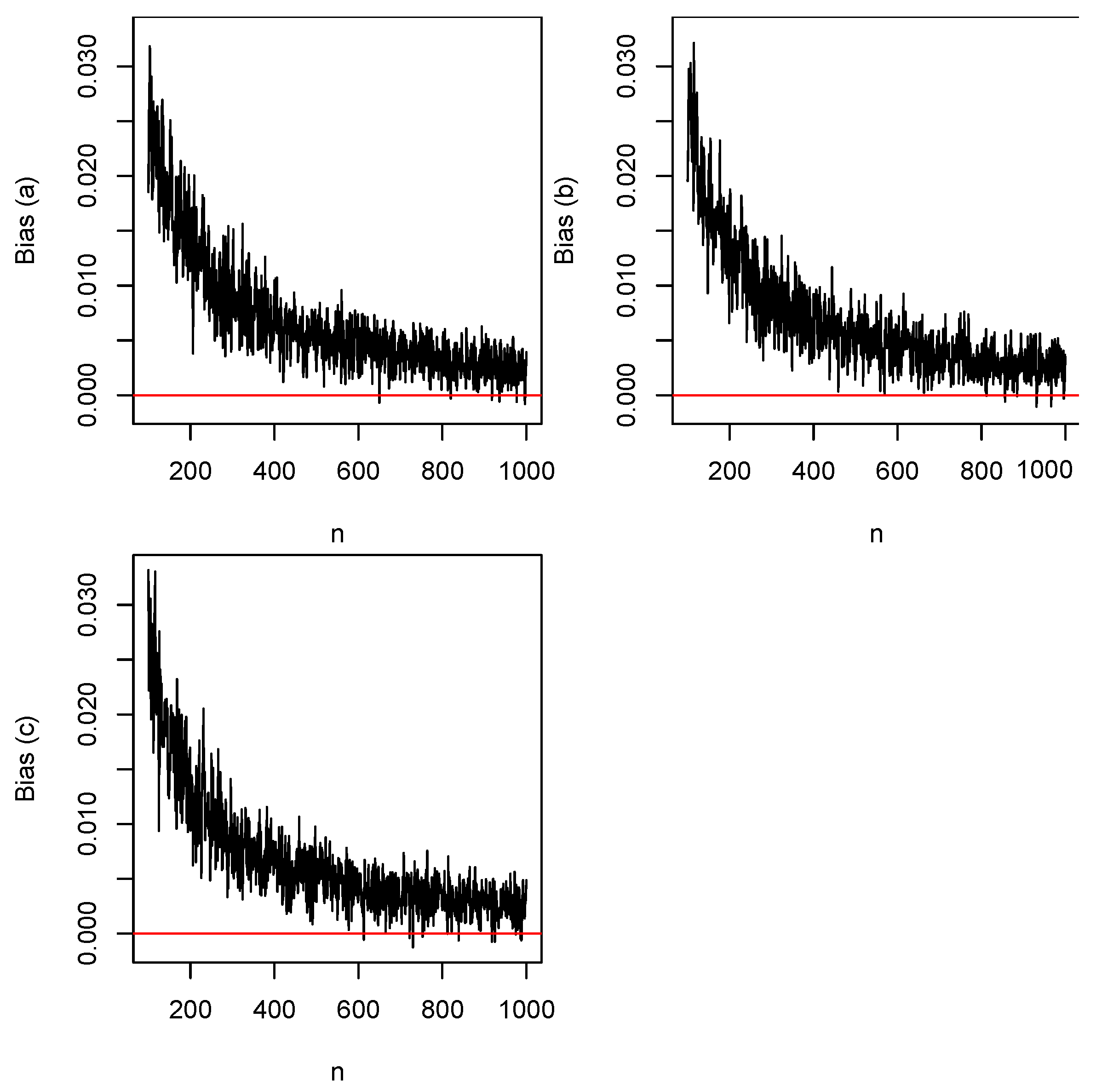
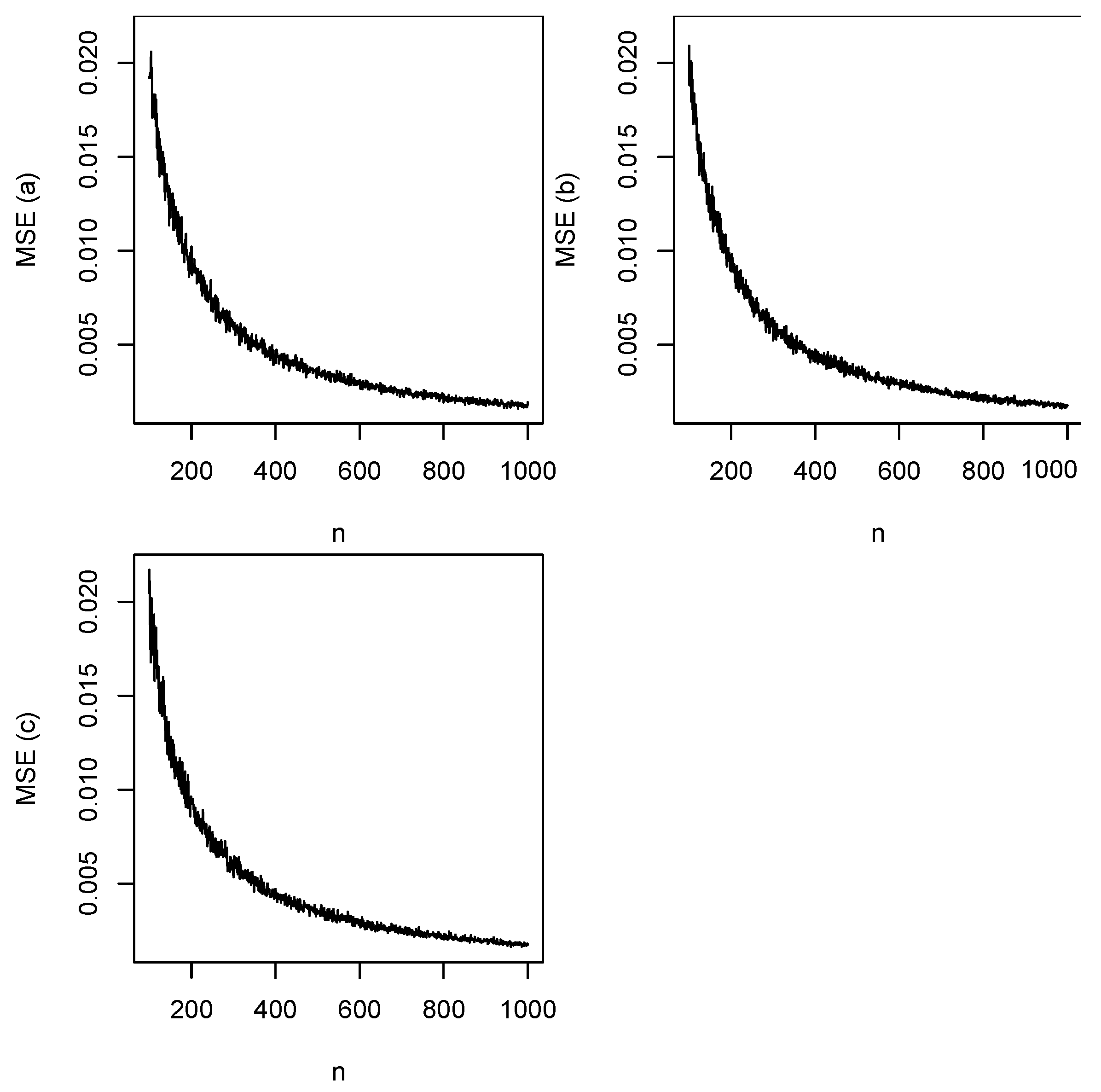
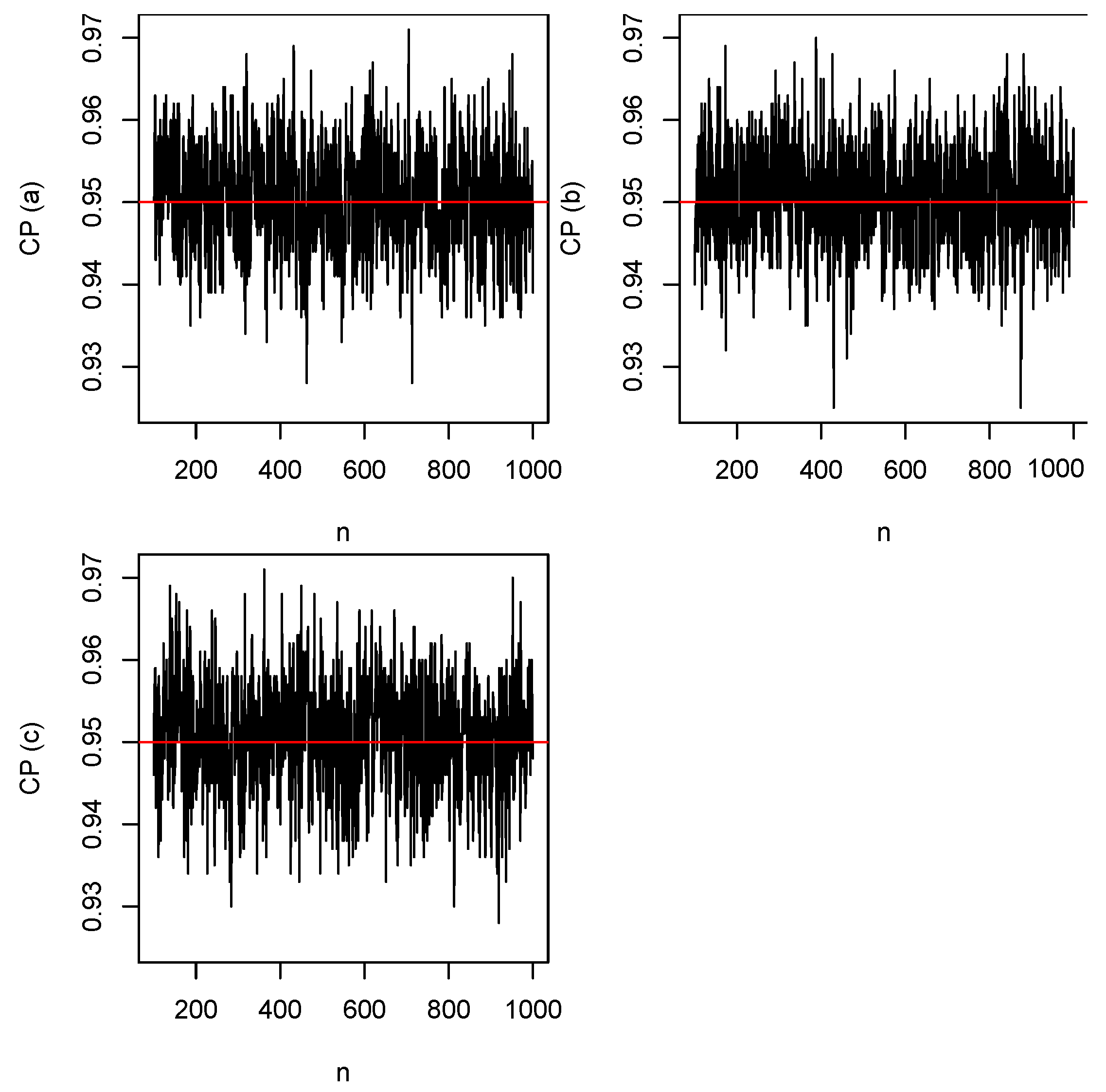
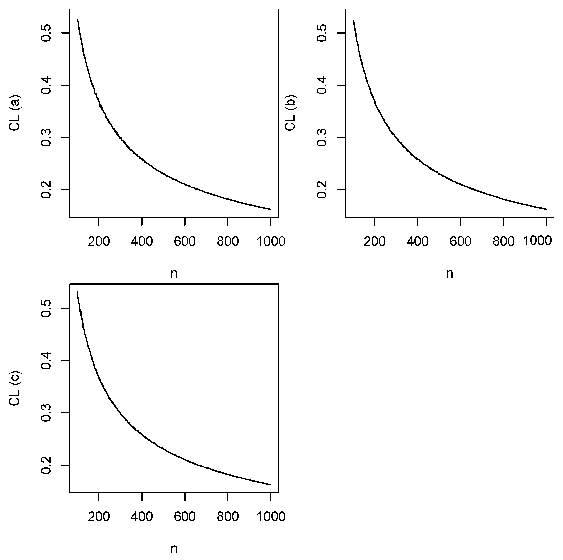
We took the initial values as a = 2 , b = 2 , and c = 1 . Plots of the biases versus n are shown in Figure 2. The horizontal lines in this figure correspond to the biases being zero. Plots of the mean squared errors versus n are shown in Figure 3. Plots of the coverage probabilities versus n are shown in Figure 4. The horizontal lines in this figure correspond to the coverage probabilities being equal to 0.95. Plots of the coverage lengths versus n are shown in Figure 5.
We can observe the following from the figures:
(a)
The biases are generally positive and decrease to zero with increasing n;
(b)
The mean squared errors generally decrease to zero with increasing n;
(c)
The coverage probabilities are around the nominal level even for n as small as 100;
(d)
The coverage lengths generally decrease to zero with increasing n.
The observations noted are for particular initial values of a, b, and c, but the same observations held for a wide range of other values of a, b, and c, including the ones corresponding to the different shapes in Figure 1. We chose not to present results for other choices in order to save space and to avoid repetitive discussion. In particular, the biases always decreased to zero with increasing n, the mean squared errors always decreased to zero with increasing n, the coverage probabilities were always around the nominal level even for n as small as 100, and the coverage lengths always decreased to zero with increasing n.

12. Real Data Applications

In this section, we compare the performance of the confluent hypergeometric beta distribution versus competing distributions using two real datasets. In Section 12.1, the confluent hypergeometric beta distribution is compared with the standard beta distribution. In Section 12.2, the confluent hypergeometric beta distribution is compared with [15]’s beta distribution specified by the probability density function
f ( x ) = c a x a 1 ( 1 x ) b 1 B ( a , b ) 1 ( 1 c ) x a + b
for 0 < x < 1 , a > 0 , b > 0 , and c > 0 . The method of maximum likelihood was used to fit all of the distributions.

12.1. United States Presidential Elections Data

The data used are the winner’s share of the electoral college vote for the United States presidential elections from 1824 to 2016. The actual data values are 0.3218, 0.6820, 0.7657, 0.5782, 0.7959, 0.6182, 0.5621, 0.8581, 0.5878, 0.5941, 0.9099, 0.7279, 0.8125, 0.5014, 0.5799, 0.5461, 0.5810, 0.6239, 0.6063, 0.6523, 0.7059, 0.6646, 0.8192, 0.5217, 0.7608, 0.7194, 0.8362, 0.8889, 0.9849, 0.8456, 0.8136, 0.5706, 0.8324, 0.8606, 0.5642, 0.9033, 0.5595, 0.9665, 0.5520, 0.9089, 0.9758, 0.7918, 0.6877, 0.7045, 0.5037, 0.5316, 0.6784, 0.6171, 0.5687.
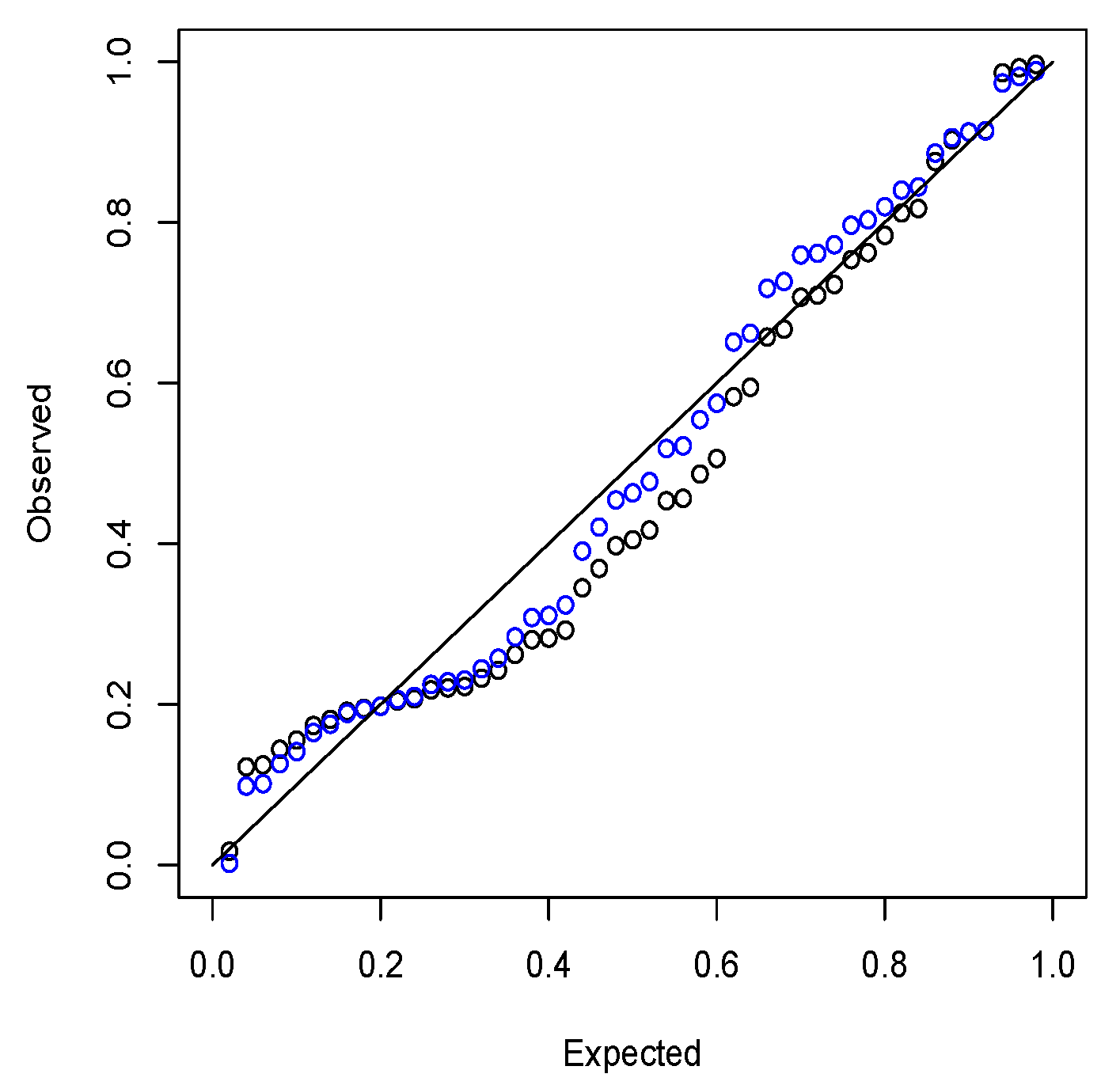
The fit of the standard beta distribution gave a ^ = 4.895 ( 0.992 ) and b ^ = 2.053 ( 0.388 ) with log L = 22.838 , where the numbers within parentheses are standard errors. The fit of (1) gave a ^ = 16.217 ( 0.049 ) , b ^ = 1.000 ( 0.035 ) , and c ^ = 22.236 ( 3.068 ) with log L = 25.990 . By the likelihood ratio test, (1) provides a significantly better fit than the standard beta distribution. In addition, the standard errors are smaller for the fit of (1).
The better fit of (1) is confirmed by the probability plots shown in Figure 6. The plotted points for (1) are closer to the diagonal line. The sum of the absolute deviations between the expected and observed probabilities for the fit of the standard beta distribution is 2.455. The same for the fit of (1) is 1.857.

12.2. Brexit Data

The data used are the proportion voting “Remain” in the Brexit (EU referendum) poll outcomes for 126 polls from January 2016 to the referendum date on June 2016. The actual data values are 0.52, 0.55, 0.49, 0.44, 0.54, 0.48, 0.41, 0.45, 0.42, 0.53, 0.45, 0.44, 0.44, 0.42, 0.42, 0.37, 0.46, 0.43, 0.39, 0.45, 0.44, 0.46, 0.40, 0.48, 0.42, 0.44, 0.45, 0.43, 0.43, 0.48, 0.41, 0.43, 0.40, 0.41, 0.42, 0.44, 0.51, 0.44, 0.44, 0.41, 0.41, 0.45, 0.55, 0.44, 0.44, 0.52, 0.55, 0.47, 0.43, 0.55, 0.38, 0.36, 0.38, 0.44, 0.42, 0.44, 0.43, 0.42, 0.49, 0.39, 0.41, 0.45, 0.43, 0.44, 0.51, 0.51, 0.49, 0.48, 0.43, 0.53, 0.38, 0.40, 0.39, 0.35, 0.45, 0.42, 0.40, 0.39, 0.44, 0.51, 0.39, 0.35, 0.41, 0.51, 0.45, 0.49, 0.40, 0.48, 0.41, 0.46, 0.47, 0.43, 0.45, 0.48, 0.49, 0.40, 0.40, 0.40, 0.39, 0.41, 0.39, 0.48, 0.48, 0.37, 0.38, 0.42, 0.51, 0.45, 0.40, 0.54, 0.36, 0.43, 0.49, 0.41, 0.36, 0.42, 0.38, 0.55, 0.44, 0.54, 0.41, 0.52, 0.42, 0.38, 0.42, 0.44.
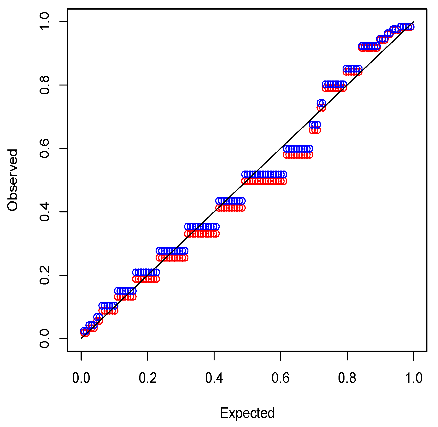
The fit of [15]’s beta distribution gave a ^ = 3.866 × 10 6 ( 2.048 ) , b ^ = 27.119 ( 0.462 ) , and c ^ = 183838.1 ( 1.192 ) with log L = 204.054 . The fit of (1) gave a ^ = 83.087 ( 0.301 ) , b ^ = 1.000 ( 0.301 ) , and c ^ = 188.068 ( 0.912 ) with log L = 209.032 . Both (1) and (13) are not nested, but they have the same number of parameters; hence, it is sufficient to compare the loglikelihood values. Clearly, (1) gives the larger value. In addition, the standard errors are smaller for the fit of (1).
The better fit of (1) is confirmed by the probability plots shown in Figure 7. The plotted points for (1) are closer to the diagonal line except in the upper tail.

13. Conclusions

In this paper, we revisited the confluent hypergeometric beta distribution introduced by [1] and derived various mathematical properties of it. Some of the derived properties are known, but most of the derived properties are new. In particular, shape properties of the probability density function, expression for the cumulative distribution function, expression for the hazard rate and reversed hazard rate functions, expressions for the moment generating and characteristic functions, expressions for harmonic means, expressions for the variances of inverse confluent hypergeometric beta random variables, expressions for conditional moments, expressions for geometric mean, Shannon entropy, Rényi entropy, relative entropy, geometric variances and geometric covariance, stochastic ordering properties, and procedures for maximum likelihood estimation are all new. We also assessed the finite sample performance of maximum likelihood estimators and illustrated two real data applications.
Future work will consider methods of estimation other than the method of maximum likelihood, including Bayesian method, method of moments, generalized method of moments, method of probability weighted moments, method of least squares, method of weighted least squares, method of maximum entropy, method of pseudo maximum likelihood, method of minimum chi-square, method of minimum L p norm, method of min–max, method of M-estimation, method of quantiles, method of ranked set sampling, and bootstrap method. Another aim is to study mathematical properties of composite beta distributions of the kind due to [16].

Author Contributions

Methodology, S.N.; Software, S.N. and M.K.; Formal analysis, M.K.; Writing—original draft, S.N.; Supervision, S.N. All authors have read and agreed to the published version of the manuscript.

Funding

This paper has received no external funding.

Institutional Review Board Statement

Not applicable.

Informed Consent Statement

Not applicable.

Data Availability Statement

Data are given as part of the manuscript. Code can be obtained from the corresponding author.

Acknowledgments

The authors would like to thank the Editor and the four referees for careful reading and comments which greatly improved the paper.

Conflicts of Interest

The authors declare no conflict of interest.

Appendix A. Second-Order Partial Derivatives of (12)

The second-order partial derivatives of (12) are
2 log L a 2 = n K 2 K a 2 n K 2 K a 2 ,
2 log L a b = n K 2 K a b n K 2 K a K b ,
2 log L a c = n K 2 K a c n K 2 K a K c ,
2 log L b 2 = n K 2 K b 2 n K 2 K b 2 ,
2 log L b c = n K 2 K b c n K 2 K b K c
and
2 log L c 2 = n K 2 K c 2 n K 2 K c 2 ,
where
2 K a 2 = 2 K K a Γ ( a ) Γ ( b ) Γ ( a + b ) 1 F 1 a ;   a + b ;   c K 2 Γ ( a ) Γ ( b ) Γ ( a + b ) 1 F 1 a ;   a + b ;   c K 2 Γ ( a ) Γ ( b ) Γ ( a + b ) 1 F 1 a ;   a + b ;   c a + K 2 Γ ( a ) Γ ( b ) Γ ( a + b ) Γ ( a + b ) 2 1 F 1 a ;   a + b ;   c 2 K K a Γ ( a ) Γ ( b ) Γ ( a + b ) 1 F 1 a ;   a + b ;   c a K 2 Γ ( a ) Γ ( b ) Γ ( a + b ) 1 F 1 a ;   a + b ;   c a K 2 Γ ( a ) Γ ( b ) Γ ( a + b ) 2 1 F 1 a ;   a + b ;   c a 2 + K 2 Γ ( a ) Γ ( b ) Γ ( a + b ) Γ ( a + b ) 2 1 F 1 a ;   a + b ;   c a + 2 K K a Γ ( a ) Γ ( b ) Γ ( a + b ) Γ ( a + b ) 2 1 F 1 a ;   a + b ;   c + K 2 Γ ( a ) Γ ( b ) Γ ( a + b ) Γ ( a + b ) 2 1 F 1 a ;   a + b ;   c + K 2 Γ ( a ) Γ ( b ) Γ ( a + b ) Γ ( a + b ) 2 1 F 1 a ;   a + b ;   c + K 2 Γ ( a ) Γ ( b ) Γ ( a + b ) Γ ( a + b ) 2 1 F 1 a ;   a + b ;   c a 2 K 2 Γ ( a ) Γ ( b ) Γ ( a + b ) 2 Γ ( a + b ) 3 1 F 1 a ;   a + b ;   c ,
2 K a b = 2 K K b Γ ( a ) Γ ( b ) Γ ( a + b ) 1 F 1 a ;   a + b ;   c K 2 Γ ( a ) Γ ( b ) Γ ( a + b ) 1 F 1 a ;   a + b ;   c K 2 Γ ( a ) Γ ( b ) Γ ( a + b ) 1 F 1 a ;   a + b ;   c b + K 2 Γ ( a ) Γ ( b ) Γ ( a + b ) Γ ( a + b ) 2 1 F 1 a ;   a + b ;   c 2 K K b Γ ( a ) Γ ( b ) Γ ( a + b ) 1 F 1 a ;   a + b ;   c a K 2 Γ ( a ) Γ ( b ) Γ ( a + b ) 1 F 1 a ;   a + b ;   c a K 2 Γ ( a ) Γ ( b ) Γ ( a + b ) 2 1 F 1 a ;   a + b ;   c a b + K 2 Γ ( a ) Γ ( b ) Γ ( a + b ) Γ ( a + b ) 2 1 F 1 a ;   a + b ;   c a + 2 K K a Γ ( a ) Γ ( b ) Γ ( a + b ) Γ ( a + b ) 2 1 F 1 a ;   a + b ;   c + K 2 Γ ( a ) Γ ( b ) Γ ( a + b ) Γ ( a + b ) 2 1 F 1 a ;   a + b ;   c + K 2 Γ ( a ) Γ ( b ) Γ ( a + b ) Γ ( a + b ) 2 1 F 1 a ;   a + b ;   c + K 2 Γ ( a ) Γ ( b ) Γ ( a + b ) Γ ( a + b ) 2 1 F 1 a ;   a + b ;   c b 2 K 2 Γ ( a ) Γ ( b ) Γ ( a + b ) 2 Γ ( a + b ) 3 1 F 1 a ;   a + b ;   c ,
2 K a c = 2 K K c Γ ( a ) Γ ( b ) Γ ( a + b ) 1 F 1 a ;   a + b ;   c K 2 Γ ( a ) Γ ( b ) Γ ( a + b ) 1 F 1 a ;   a + b ;   c c 2 K K c Γ ( a ) Γ ( b ) Γ ( a + b ) 1 F 1 a ;   a + b ;   c a K 2 Γ ( a ) Γ ( b ) Γ ( a + b ) 2 1 F 1 a ;   a + b ;   c a c + 2 K K c Γ ( a ) Γ ( b ) Γ ( a + b ) Γ ( a + b ) 2 1 F 1 a ;   a + b ;   c + K 2 Γ ( a ) Γ ( b ) Γ ( a + b ) Γ ( a + b ) 2 1 F 1 a ;   a + b ;   c c ,
2 K b 2 = 2 K K b Γ ( b ) Γ ( a ) Γ ( a + b ) 1 F 1 a ;   a + b ;   c K 2 Γ ( b ) Γ ( a ) Γ ( a + b ) 1 F 1 a ;   a + b ;   c K 2 Γ ( b ) Γ ( a ) Γ ( a + b ) 1 F 1 a ;   a + b ;   c b + K 2 Γ ( b ) Γ ( a ) Γ ( a + b ) Γ ( a + b ) 2 1 F 1 a ;   a + b ;   c 2 K K b Γ ( a ) Γ ( b ) Γ ( a + b ) 1 F 1 a ;   a + b ;   c b K 2 Γ ( b ) Γ ( a ) Γ ( a + b ) 1 F 1 a ;   a + b ;   c b K 2 Γ ( a ) Γ ( b ) Γ ( a + b ) 2 1 F 1 a ;   a + b ;   c b 2 + K 2 Γ ( a ) Γ ( b ) Γ ( a + b ) Γ ( a + b ) 2 1 F 1 a ;   a + b ;   c b + 2 K K b Γ ( a ) Γ ( b ) Γ ( a + b ) Γ ( a + b ) 2 1 F 1 a ;   a + b ;   c + K 2 Γ ( b ) Γ ( a ) Γ ( a + b ) Γ ( a + b ) 2 1 F 1 a ;   a + b ;   c + K 2 Γ ( a ) Γ ( b ) Γ ( a + b ) Γ ( a + b ) 2 1 F 1 a ;   a + b ;   c + K 2 Γ ( a ) Γ ( b ) Γ ( a + b ) Γ ( a + b ) 2 1 F 1 a ;   a + b ;   c b 2 K 2 Γ ( a ) Γ ( b ) Γ ( a + b ) 2 Γ ( a + b ) 3 1 F 1 a ;   a + b ;   c ,
2 K b c = 2 K K c Γ ( b ) Γ ( a ) Γ ( a + b ) 1 F 1 a ;   a + b ;   c K 2 Γ ( b ) Γ ( a ) Γ ( a + b ) 1 F 1 a ;   a + b ;   c c 2 K K c Γ ( a ) Γ ( b ) Γ ( a + b ) 1 F 1 a ;   a + b ;   c b K 2 Γ ( a ) Γ ( b ) Γ ( a + b ) 2 1 F 1 a ;   a + b ;   c b c + 2 K K c Γ ( a ) Γ ( b ) Γ ( a + b ) Γ ( a + b ) 2 1 F 1 a ;   a + b ;   c + K 2 Γ ( a ) Γ ( b ) Γ ( a + b ) Γ ( a + b ) 2 1 F 1 a ;   a + b ;   c c
and
2 K c 2 = 2 K K c 1 F 1 a ;   a + b ;   c c K 2 2 1 F 1 a ;   a + b ;   c c 2 .

References

  1. Gordy, M.B. Computationally convenient distributional assumptions for common-value auctions. Comput. Econ. 1998, 12, 61–78. [Google Scholar] [CrossRef]
  2. Nadarajah, S. Exponentiated beta distributions. Comput. Math. Appl. 2005, 49, 1029–1035. [Google Scholar] [CrossRef]
  3. Li, Y.; Clyde, M.A. Mixtures of g-priors in generalized linear models. J. Am. Stat. Assoc. 2018, 113, 1828–1845. [Google Scholar] [CrossRef]
  4. Sarabia, M.J.; Shahtahmassebi, G. Bayesian estimation of incomplete data using conditionally specified priors. Commun. Stat. Simul. Comput. 2017, 46, 3419–3435. [Google Scholar] [CrossRef]
  5. Alshkaki, R.S.A. A six parameters beta distribution with application for modeling waiting time of Muslim early morning prayer. Ann. Data Sci. 2021, 8, 57–90. [Google Scholar] [CrossRef]
  6. Gradshteyn, I.S.; Ryzhik, I.M. Table of Integrals, Series, and Products, 6th ed.; Academic Press: San Diego, CA, USA, 2000. [Google Scholar]
  7. Prudnikov, A.; Brychkov, Y.A.; Marichev, I.O. Integrals and Series; Gordon and Breach Science Publishers: Amsterdam, The Netherlands, 1986; Volumes 1–3. [Google Scholar]
  8. Feng, C.; Wang, H.; Tu, X.M. Geometric mean of nonnegative random variable. Commun. Stat. Theory Methods 2013, 42, 2714–2717. [Google Scholar] [CrossRef]
  9. Vogel, R.M. The geometric mean? Commun. Stat. Theory Methods. 2022, 51, 82–94. [Google Scholar] [CrossRef]
  10. Shannon, C.E. A mathematical theory of communication. Bell Syst. Tech. J. 1948, 27, 379–423. [Google Scholar] [CrossRef]
  11. Shannon, C.E. A mathematical theory of communication. Bell Syst. Tech. J. 1948, 27, 623–656. [Google Scholar] [CrossRef]
  12. Rényi, A. On measures of information and entropy. In Proceedings of the 4th Berkeley Symposium on Mathematics, Statistics and Probability; Neyman, J., Ed.; University of California Press: Berkeley, CA, USA, 1960; Volume 1, pp. 547–561. [Google Scholar]
  13. Kullback, S.; Leibler, R.A. On information and sufficiency. Ann. Math. Stat. 1951, 22, 79–86. [Google Scholar] [CrossRef]
  14. R Core Team. R: A Language and Environment for Statistical Computing; R Foundation for Statistical Computing: Vienna, Austria, 2023. [Google Scholar]
  15. Libby, L.D.; Novick, R.M. Multivariate generalized beta-distributions with applications to utility assessment. J. Educ. Stat. 1982, 7, 271–294. [Google Scholar] [CrossRef]
  16. Zaevski, T.; Kyurkchiev, N. On some composite Kies families: Distributional properties and saturation in Hausdorff sense. Mod. Stoch. Theory Appl. 2023, 1–26. [Google Scholar] [CrossRef]
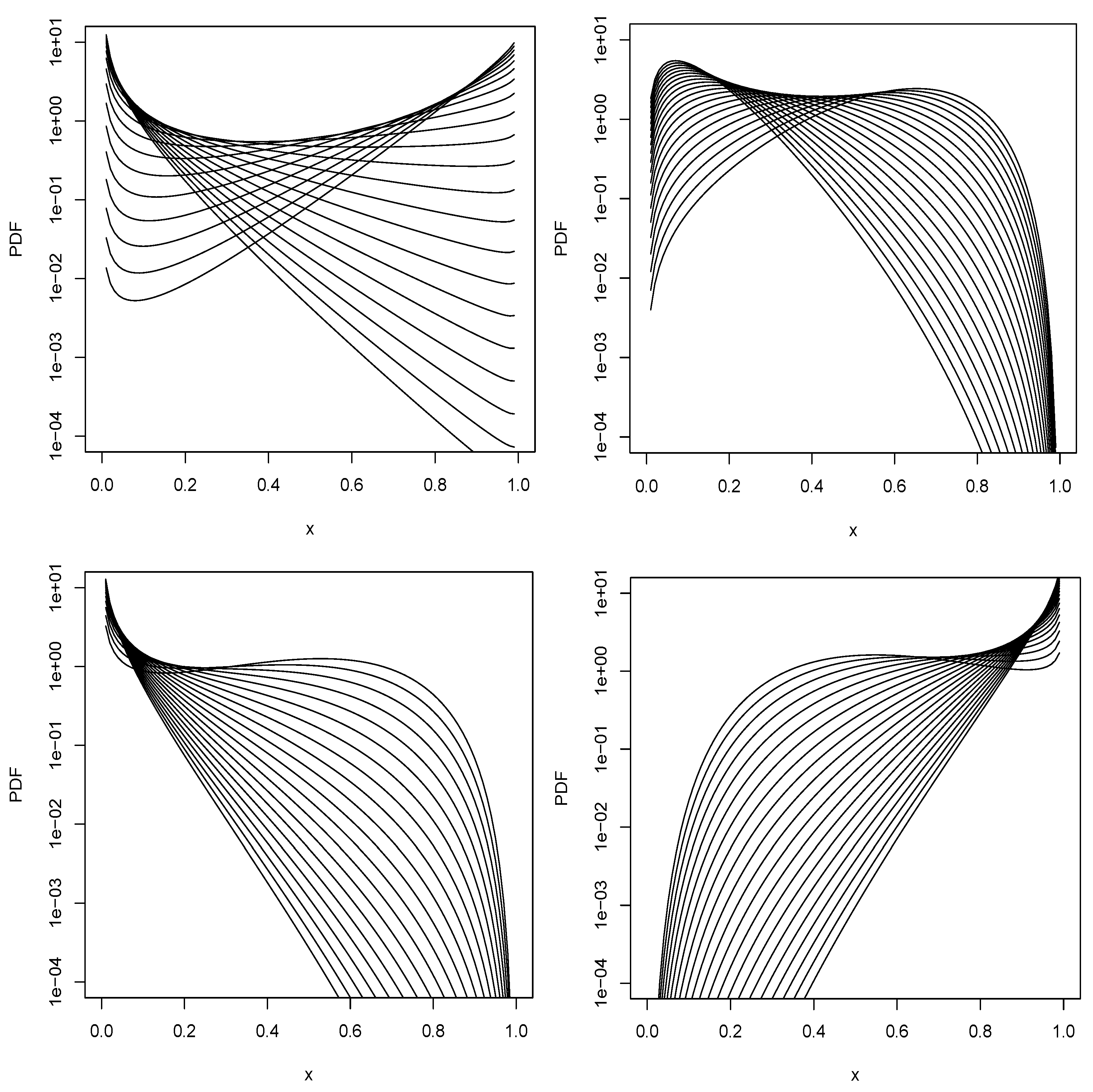
Figure 1. Shapes of (1) for a = 0.2 , b = 0.9 and c = 10 , 9 , , 10 (top left); a = 2 , b = 5 , and c = 10 , 9 , , 10 (top right); a = 0.2 , b = 5 , and c = 10 , 9 , , 10 (bottom left); a = 6 , b = 0.6 , and c = 10 , 9 , , 10 (bottom right). The curves from the top to bottom on the right hand side of each plot correspond to c = 10 , 9 , , 10 .
Mathematics 11 02169 g001
Figure 2. Biases of a ^ (top left), b ^ (top right), and c ^ (bottom left) versus n. The horizontal lines correspond to the biases being zero.
Mathematics 11 02169 g002
Figure 3. Mean squared errors of a ^ (top left), b ^ (top right), and c ^ (bottom left) versus n.
Mathematics 11 02169 g003
Figure 4. Coverage probabilities of a ^ (top left), b ^ (top right), and c ^ (bottom left) versus n. The horizontal lines correspond to the coverage probabilities being equal to 0.95.
Mathematics 11 02169 g004
Figure 5. Coverage lengths of a ^ (top left), b ^ (top right), and c ^ (bottom left) versus n.
Mathematics 11 02169 g005
Figure 6. Probability plots of the fits of the standard beta (black) and confluent hypergeometric beta (blue) distributions.
Mathematics 11 02169 g006
Figure 7. Probability plots of the fits of [15]’s beta (red) and confluent hypergeometric beta (blue) distributions.
Mathematics 11 02169 g007
Disclaimer/Publisher’s Note: The statements, opinions and data contained in all publications are solely those of the individual author(s) and contributor(s) and not of MDPI and/or the editor(s). MDPI and/or the editor(s) disclaim responsibility for any injury to people or property resulting from any ideas, methods, instructions or products referred to in the content.