Article

Solving Stochastic Nonlinear Poisson-Boltzmann Equations Using a Collocation Method Based on RBFs

1
Faculty of Mathematical Sciences, Shahrood University of Technology, Shahrood 36199-95161, Iran
2
Department of Mathematical Sciences, Isfahan University of Technology, Isfahan 84156-83111, Iran
3
Institute of Analysis and Scientific Computing, TU Wien, 1040 Vienna, Austria
*
Author to whom correspondence should be addressed.
Mathematics 2023, 11(9), 2118; https://doi.org/10.3390/math11092118
Submission received: 30 March 2023 / Revised: 22 April 2023 / Accepted: 24 April 2023 / Published: 29 April 2023
(This article belongs to the Special Issue Stochastic Processes: Theory, Simulation and Applications)

Abstract

:
In this paper, we present a numerical scheme based on a collocation method to solve stochastic non-linear Poisson–Boltzmann equations (PBE). This equation is a generalized version of the non-linear Poisson–Boltzmann equations arising from a form of biomolecular modeling to the stochastic case. Applying the collocation method based on radial basis functions (RBFs) allows us to deal with the difficulties arising from the complexity of the domain. To indicate the accuracy of the RBF method, we present numerical results for two-dimensional models, we also study the stability of this method numerically. We examine our results with the RBF-reference value and the Chebyshev Spectral Collocation (CSC) method. Furthermore, we discuss finding the appropriate shape parameter to obtain an accurate numerical solution besides greatest stability. We have exerted the Newton–Raphson approach for solving the system of non-linear equations resulting from discretization by the RBF technique.

1. Introduction

There are numerous numerical methods for solving partial differential equations (PDEs). A popular category of numerical techniques is called mesh-free methods [1,2]. As a special case of the mesh-free methods, we recall radial basis functions (RBFs) collocation methods, which recently have been studied to solve a large number of PDEs related to science and engineering problems [3,4,5,6]. The implementation of RBF methods is very simple because the main property of the RBF method is that in order to discretize it does not require a mesh, indeed it only requires setting collocation points which allow us to deal with complicated domains. Furthermore, the implementation of this method is easy for higher dimensional problems [7,8,9]. So far, many authors have published papers on the improvement of the RBF method or on how to implement the method for various PDE problems [10,11,12]. It is worth noting that this method has been applied to the study of several biological systems [13,14]. We refer interested readers to [15] for new advances in RBF methods. Several radial basis functions have been defined so far, and some of them depend on a constant which is called a shape parameter c > 0 . Some popular RBFs are collected in Table 1.
The accuracy and stability of the numerical results obtained using the collocation method are highly dependent on the choice of the collocation points and the shape parameter. A smaller shape parameter generally improves the accuracy, but it may lead to instability. Thus, there exists a trade-off between the stability and accuracy of the approximation, and determining the best shape parameter remains a challenging problem. Consequently, the value of the shape parameter is included in the unknowns and needs to be determined. The shape parameter that leads to the lowest error is called the optimal shape parameter. Various techniques have been proposed by researchers to find the optimal shape parameter [16,17,18,19,20]. When describing some physical phenomena in the form of partial differential equations, adding stochastic factors enables the achieving of a more accurate model. In recent years, many researchers have become interested in studying stochastic models [21,22]. In this work, we apply a collocation method based on radial basis functions to find the discrete solutions of a stochastic non-linear Poisson–Boltzmann equation. This class of stochastic PDEs plays a role in describing various biological phenomena, making it imperative to solve these equations to obtain beneficial solutions. This strong motivation drives us to tackle these complex equations [23,24,25]. Here, we consider the model that is described in [26].
The main focus of this paper is to propose a formulation based on the RBF collocation method to solve stochastic non-linear Poisson–Boltzmann equations. Section 2 is devoted to describing a physical model for the non-linear stochastic non-linear Poisson–Boltzmann equation. In Section 3, we present the main results of this paper which is to implement the RBF collocation method to solve our model problem. In Section 4, we present numerical results, and in the final section we have summarized the conclusions.

2. The Stochastic Non-Linear Poisson–Boltzmann Equation

Let D be an open-bounded Lipschitz domain in R d consisting of two non-overlapping sub-domains with different physical properties with the boundary D . In this paper, we assume D : = D L D M where D L contains a solvent, such as an electrolyte, blood, or salty water, and D M is the impenetrable molecules region. The domain D L is filled with two free charge carriers, namely a positive and a negative carrier (see Figure 1). We also assume P : = ( Ω , Σ , P ) is a probability space.
The above process can be described by a deterministic Poisson–Boltzmann equation. This model could be generalized to a stochastic version when the molecules move randomly inside the solvent, which is controlled by Brownian motion. Here, the movements of the molecules are independent of each other. The governing equation for the stochastic Poisson–Boltzmann equation is considered as follows
· ( a ( x , ω ) u ( x , ω ) ) + b ( x , ω , u ( x , ω ) ) = f ( x , ω ) in D L ,
· ( a ( x , ω ) u ( x , ω ) ) = g ( x , ω ) in D M ,
u ( x , ω ) = u D ( x , ω ) on D ,
where the elliptic operator depends on some coefficients a ( x , ω ) for x D and the sample ω Ω . Additionally, the force terms f ( x , ω ) and g ( x , ω ) are assumed to be random. One of the interesting cases of (1a)–(1c) is the following stochastic non-linear Poisson–Boltzmann equation
· ( a ( x , ω ) u ( x , ω ) ) + κ ( x ) sinh β u ( x , ω ) = 0 in D L ,
· ( a ( x , ω ) u ( x , ω ) ) = ρ ( x , ω ) in D M ,
u ( x , ω ) = u D ( x , ω ) on D ,
where u describes the electrostatic potential which is due to free charges, a ( x , ω ) is the dielectric constant or permittivity function, and ρ ( x , ω ) represents the fixed charges of the molecules. Here, κ ( x ) is the ionic concentration. κ ( x ) , a ( x , ω ) are the piecewise constant functions as below
a ( x , ω ) = a M x D M , a L x D L , κ ( x ) = 0 x D M , κ ¯ x D L .
β is defined as β : = q k B T , where the constants κ B , T, and q > 0 are the Boltzmann constant, the temperature, and the elementary charge, respectively.
This stochastic generalization describes physical systems where the fixed charges have probability distributions, and, hence, the electrostatic potential u is stochastic. The different configurations of the fixed charges are due to the movement of the molecules. In this situation, the input data vary randomly from one point of the physical domain D to another point. In reality, each point in the domain corresponds to a random variable, and the correlation between the values of any two distinct points in the domain is generally non-zero. In the model described here, the positions of subdomains are also stochastic.

3. Collocation Method Based on Radial Basis Functions for Solving

In this section, we present a collocation method based on radial basis functions to solve system (2a)–(2c). For the sake of simplicity, we rewrite the system (2a)–(2c) as
L u ( · , ω ) + G u ( · , ω ) = f ( · , ω ) in D ,
u ( x , ω ) = u D ( x , ω ) on D ,
where the linear elliptic operator L is defined as
L u ( · , ω ) : = · ( a L ( x , ω ) u ( x , ω ) ) x D L · ( a M ( x , ω ) u ( x , ω ) ) x D M ,
the function G is a Lipschitz continuous function defined as
G u ( · , ω ) : = κ ( x ) sinh β u ( x , ω ) x D L 0 x D M ,
and the source term f : = ( x , ω ) : = 0 x D L ρ ( x , ω ) x D M .
Let φ ( r ) : [ 0 , ) R be a type of radial basis functions defined by φ j ( x ) : = φ ( x x j ) at the collocation points { x j } j = 1 n belonging to D ¯ : = D D . We approximate u by u ˜ defined as a linear combination of the radial basis functions φ ( · ) , i.e.,
u u ˜ ( x ) = j = 1 n λ j φ j ( x ) , x j D ¯ ,
where the first n 1 nodes belong to the interior of the domain and the last node in on the boundary of the domain. Coefficients λ j are unknown and should be determined. Thus, the collocation method to solve the system (3) and (4) can be written as find λ j R , such that
j = 1 n 1 λ j L φ ( x k x j , ω ) + G j = 1 n λ j φ j ( x ) , ω = f ( x k , ω ) for k = 1 , , n 1 j = 1 n 1 λ j L φ ( x k x j , ω ) + G j = 1 n λ j φ j ( x ) , ω = 0 for k = n ,
which leads to the following system
L φ ( x 1 x 1 ) L φ ( x 1 x 2 ) L φ ( x 1 x n ) L φ ( x 2 x 1 ) L φ ( x 2 x 2 ) L φ ( x 2 x n ) φ ( x n x 1 ) φ ( x n x 2 ) φ ( x n x n ) λ 1 λ 2 λ n + G ( λ 1 , , λ n ) = f ( x 1 ) f ( x 2 ) 0 ,
where G ( λ 1 , , λ n ) : = G j = 1 n λ j φ j ( x 1 ) G j = 1 n λ j φ j ( x 2 ) 0 , and for the sake of simplicity we drop the stochastic variable ω . We then solve the above system using Newton–Raphson’s method. Finally, we define the approximate solution of system (3) and (4) as
u ( x ) u D ( x ) + j = 1 n λ j φ j ( x ) .

4. Numerical Results

To indicate the effectiveness and efficiency of the RBF method, we present the achieved numerical results for the model equation in Section 3. Consider the 2D version of problem (2a)–(2c) that the forcing term on the right-hand side is considered a stochastic term. Then, by implementing the RBF method, the right-hand vector in system (6) would be random. For presenting numerical results consider the following assumptions and constants
u = 0 on D ,
a L = 78.4 , a M = 3.7 , κ ( x ) = 1 ,
q = 1.6 × 10 19 , κ B = 1.38 × 10 23 and T = 300 .
Additionally, consider { x i } i = 1 n being the collocation points and h = max i = 1 i n x x i for all x D D . At first, we present our results for the problem consist of one molecule domain. We provide numerical results using some types of radial basis functions, such as the Multiquadric (MQ), Inverse Multiquadric (IMQ), and Inverse Quadratic (IQ) functions.
There is no exact solution for this model. Once we make sure the algorithm is correct, then we consider the approximation solution for 100 interpolation points using the MQ function as a reference value, which is shown in Figure 2.
Also, for evaluating our results by using the RBF method, we compare our results with the Chebyshev Spectral Collocation (CSC) method. In this approach, the numerical solution is interpolated using Lagrange polynomials at the roots of the derivative of Chebyshev polynomials. The interested reader is referred to [27] for detailed descriptions of the method. We consider the root-mean-square errors
RMSE : = E ( u u ˜ L 2 2 ) 1 2 ,
where u can be considered the RBF-reference value (R-value) or the approximation solutions using CSC, and u ˜ is the numerical solution obtained by the RBF method. To calculate this error we employ the Monte-carlo method with 500 realizations for all numerical results.
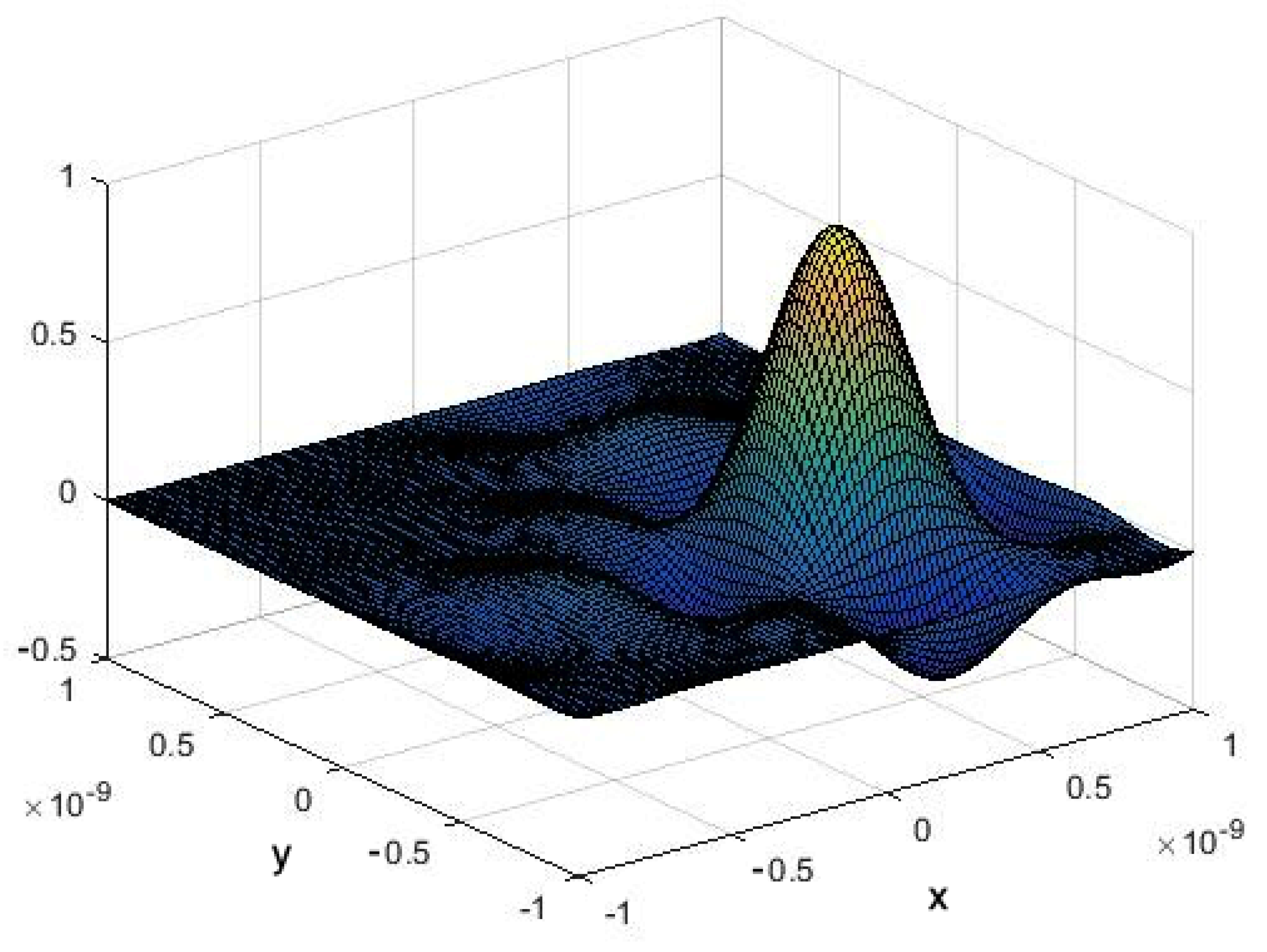
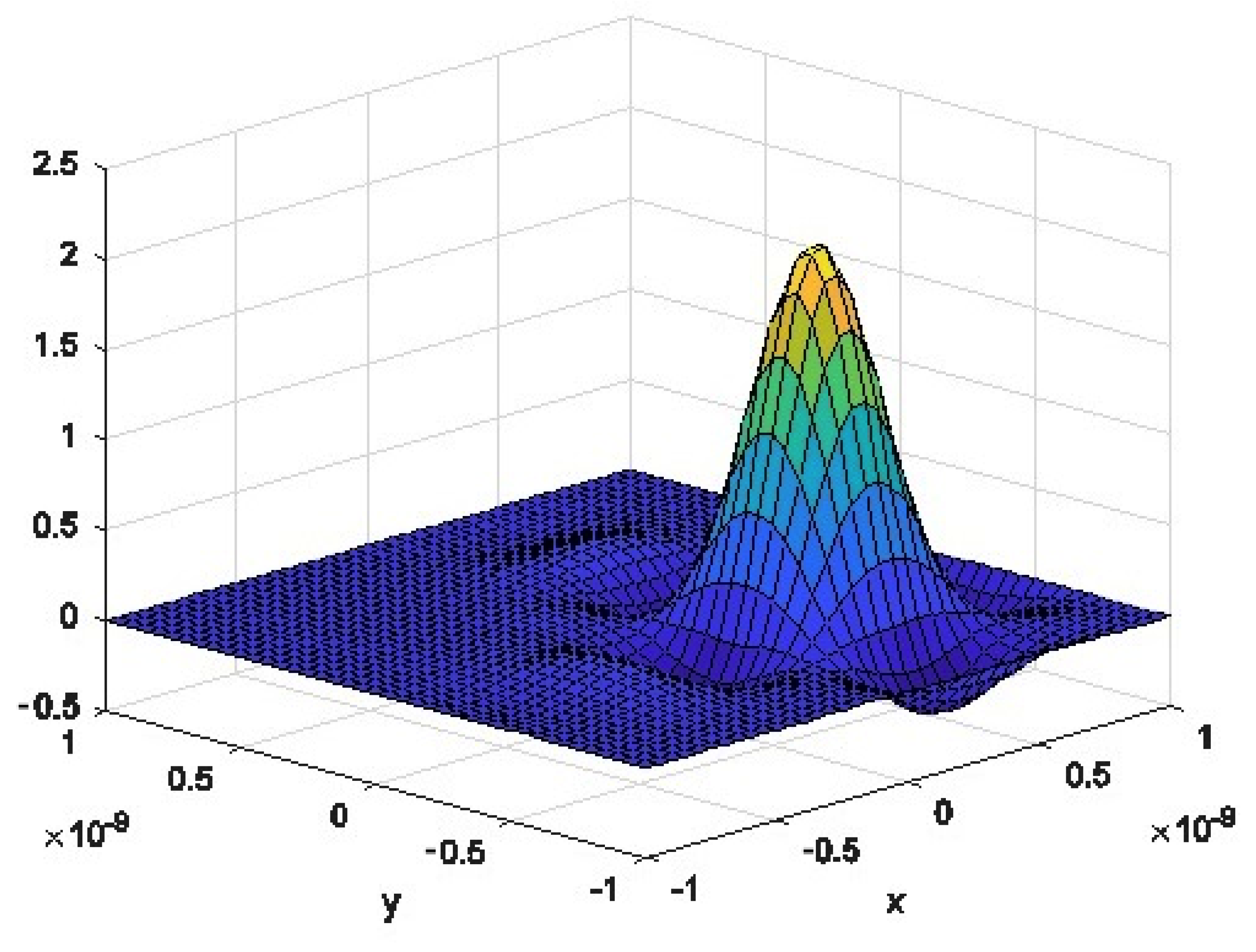
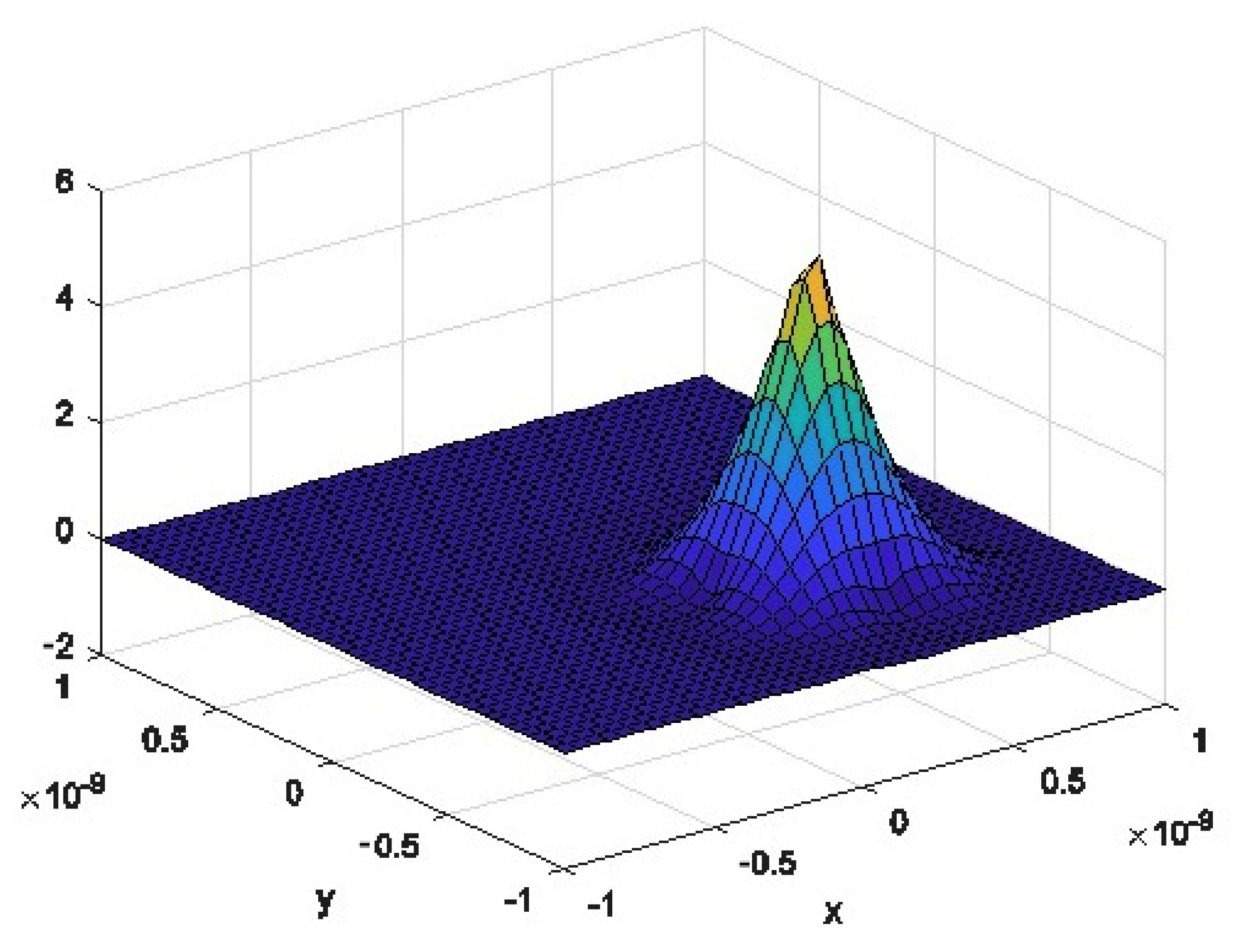
In Figure 2, it is easy to observe the electrostatic potential energy in the molecular domain D M . The potential in the liquid region D L is small. Additionally, it can be seen the nonlinearly changing near the molecule region. These observations are also visible for subsequent numerical solutions. The numerical solution and error completely depend on the value of the shape parameter c. So at first, we discuss finding an appropriate shape parameter. We survey numerical results for different shape parameters. Here, we present these results for two values of c. For this purpose, we apply the MQ function. In Figure 3 and Figure 4 we have shown the numerical solution for c = h n , c = h n 2 which using R-value estimation have RMSE 0.0169 and 0.5389 , respectively.
Hardy [28] proposed c = 0.815 d where d = 1 / n j = 1 n d j and d j is the distance of the jth collocation point from its nearest neighbor which for equispaced node we consider d = h . Additionally, we found a meaningful relation between the shape parameter, the number of interpolation points, and d, which we propose in the following formulation to reach a proper shape parameter for our method. This relation is
c = d ( n + 1 i ) , i = 1 , 2 ,
.
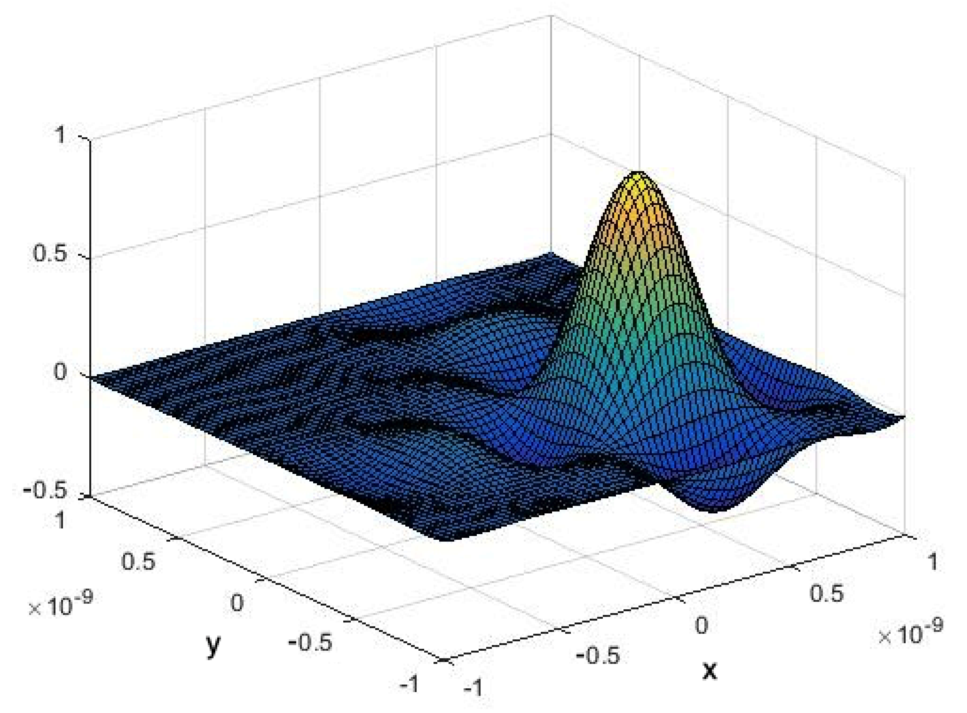
lWe gained the least RMSE = 0.0013 for the c = d n using R-value estimation. This nuemical solution is shown in Figure 5.
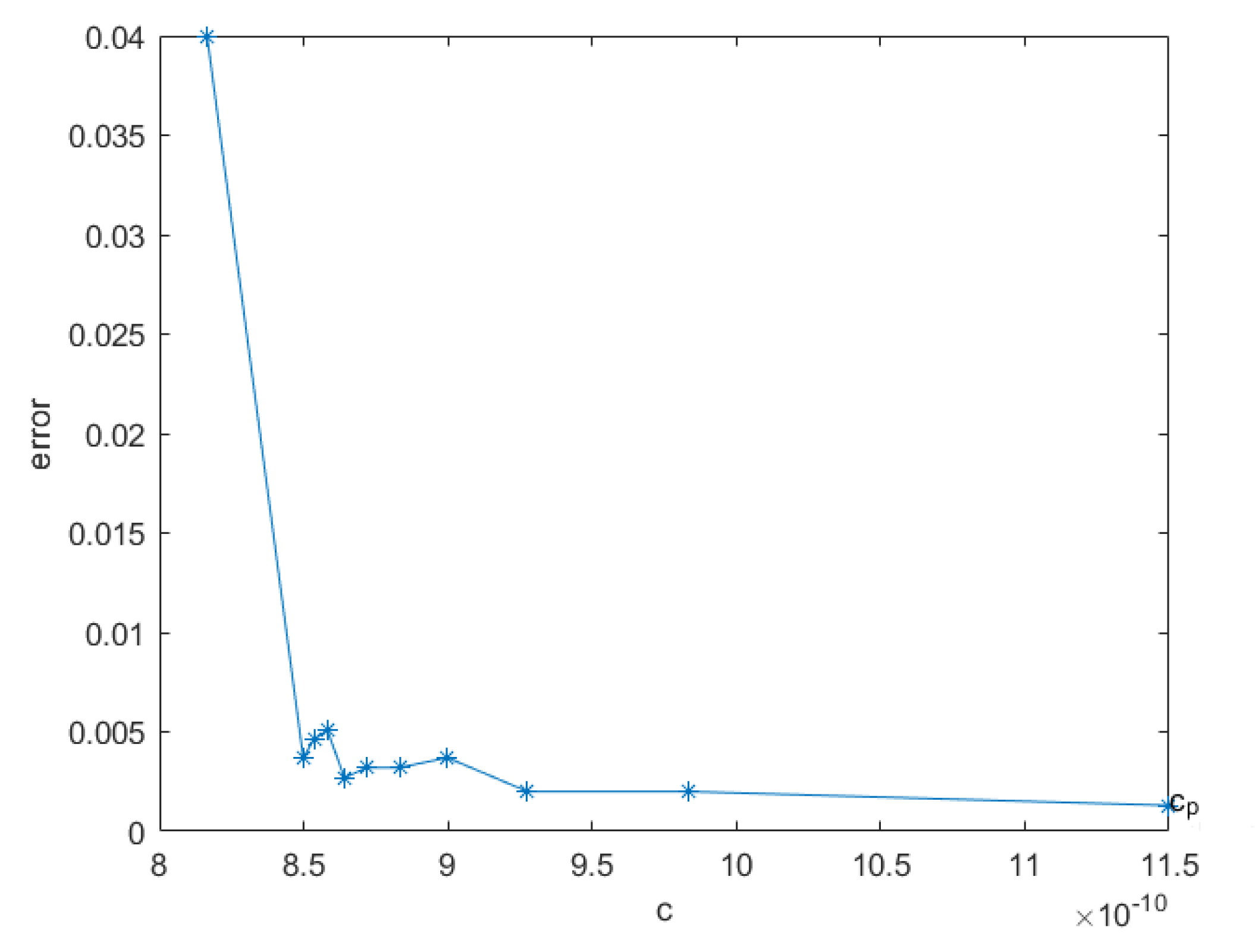
In Table 2 and Figure 6, we show RMSE for the RBF method with shape parameters gained from relation (7) for i = 1 , , 10 . These results are obtained using R-value estimation and the MQ function with n = 40.
In Table 3, we compare gained results using R-value estimation by the MQ, IMQ, and IQ function for the proposed shape parameter and shape parameter recommended by Hardy for six different runs with n = 70.
According to the results in Table 3, it is clear that the proposed shape parameter provides higher accuracy for the MQ and IMQ functions as the basis function. But using our suggested shape parameter for the IQ function does not yield quite reliable results. After finding the proper shape parameter and fixing it, we have surveyed results for various numbers of interpolation points. In Figure 7 and Figure 8, numerical solutions for n = 50 , and n = 70 by utilizing the MQ function can be seen, which via R-value estimation have RMSE = 0.0079 and 0.00027, respectively. Actually, by increasing the number of interpolation points, we could reach a more accurate approximation solution.
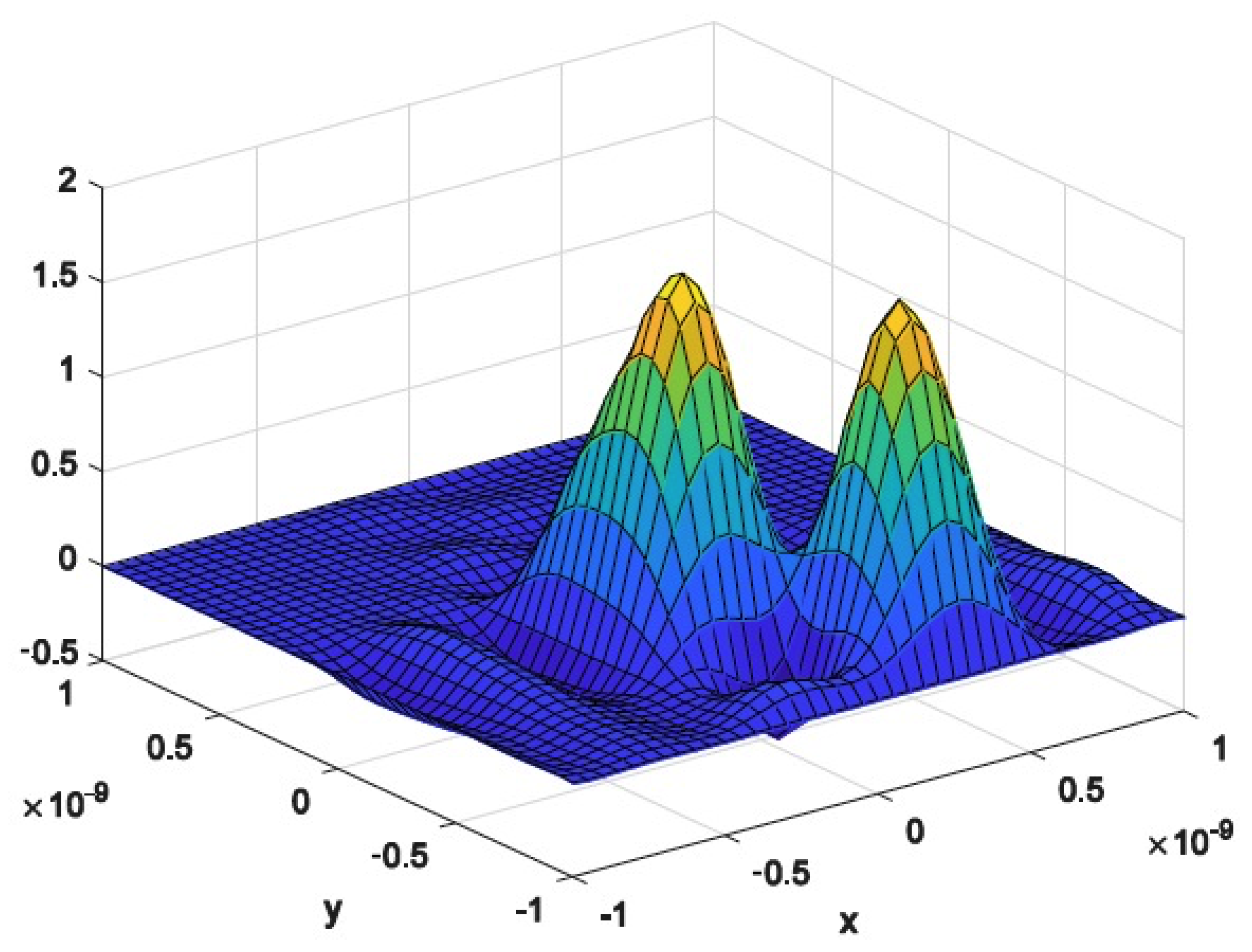
Additionally, we consider the model contains two molecules with the same assumptions of same as the first example. The implementation of the RBF method by employing the MQ function and using R-value estimation would yield RMSE = 0.0018 . Figure 9 illustrates the approximation of the numerical solution in this case.
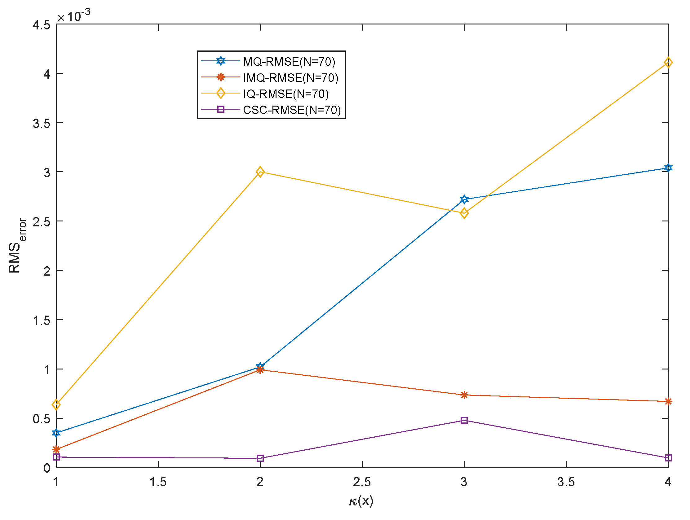
Additionally, we surveyed the numerical results for different amounts of κ ( x ) . We provided results by applying the MQ, IMQ, and IQ functions. Table 4 and Figure 10 show RMSEs by using the R-valued estimate and SCS method with n = 70 .
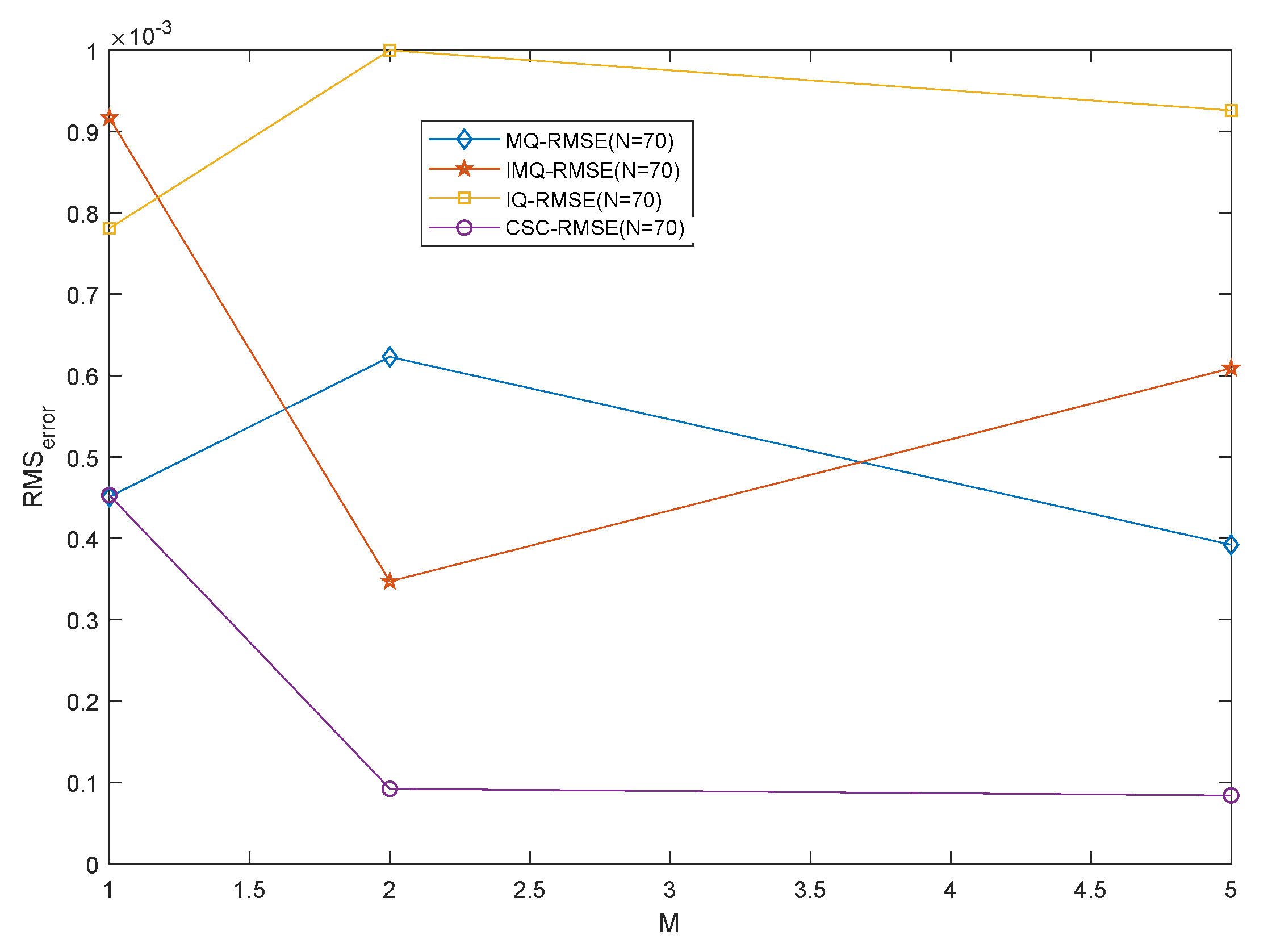
As the last case for numerical analysis, we investigated some results using the MQ, IMQ, and IQ functions for the described model including one, two, and five molecular domains ( D M ). These results are provided in Table 5 and Figure 11 by using the R-value estimation and CSC method. Figure 12 displays the numerical solution for the model includes five molecular subdomains using the MQ function with n = 70.
The proof of stability for collocation methods is difficult. More specifically for the described model in Section 3 which is non-linear and stochastic, it is even more complicated. However, there are some ways to indicate stability numerically. One of them is as follows: if by changing the shape parameter around a determined value the results do not differ much, it can be concluded that the method is stable for that shape parameter. Due to Table 2, we can observe that whatever the shape parameter would be close to our suggested shape parameter, the condition number of the matrix obtained in (6) would change only insignificantly. Therefore, this is evidence for the stability of the RBF method when employing the suggested shape parameter.

5. Conclusions

In this paper, we have thoroughly demonstrated the efficiency and performance of the RBF method for solving non-linear stochastic elliptic models. The numerical results clearly show that this method provides accurate solutions with ease. Not only is the RBF method efficient, but it is also straightforward to implement, making it more convenient than other methods, such as finite differences or finite elements. Thus, we recommend the RBF method as a powerful tool for solving non-linear stochastic equations, particularly those with complex geometry. Looking ahead, we plan to extend and improve this method for solving biological PDEs, which are often defined on complex domains. With its accuracy and simplicity, we believe the RBF method can be a valuable resource for tackling real-world problems.

Author Contributions

Conceptualization, S.M. and C.H.; Methodology, S.M.; Software, S.M. and R.A.; Validation, C.H.; Investigation, S.M.; Data curation, C.H.; Writing—original draft, S.M.; Supervision, A.M., R.M. and C.H. All authors have read and agreed to the published version of the manuscript.

Funding

This research received no external funding.

Data Availability Statement

No new data were created or analyzed in this study. Data sharing is not applicable to this article.

Conflicts of Interest

The authors declare no conflict of interest.

References

  1. Fasshauer, G.E. Meshfree methods. In Handbook of Theoretical and Computational Nanotechnology; American Scientific Publishers: Stevenson Ranch, CA, USA, 2006; Volume 27, pp. 33–97. [Google Scholar]
  2. Fasshauer, G.E. Meshfree Approximation Methods with MATLAB; World Scientific: Singapore, 2007; Volume 6. [Google Scholar]
  3. Cavoretto, R.; De Rossi, A. An adaptive loocv-based refinement scheme for rbf collocation methods over irregular domains. Appl. Math. Lett. 2020, 103, 106178. [Google Scholar] [CrossRef]
  4. Cavoretto, R.; De Rossi, A. A two-stage adaptive scheme based on rbf collocation for solving elliptic pdes. Comput. Math. Appl. 2020, 79, 3206–3222. [Google Scholar] [CrossRef]
  5. Chen, C.S.; Karageorghis, A.; Dou, F. A novel rbf collocation method using fictitious centres. Appl. Math. Lett. 2020, 101, 106069. [Google Scholar] [CrossRef]
  6. Mokhtari, R.; Ziaratgahi, S.T. Numerical solution of rlw equation using integrated radial basis functions. Appl. Comput. Math 2011, 10, 428–448. [Google Scholar]
  7. Li, M.; Chen, W.; Chen, C.S. The localized rbfs collocation methods for solving high dimensional pdes. Eng. Anal. Bound. Elem. 2013, 37, 1300–1304. [Google Scholar] [CrossRef]
  8. Li, N.; Tan, Z.; Feng, X. Novel two-level discretization method for high dimensional semilinear elliptic problems base on rbf-fd scheme. Numer. Heat Transf. Part B Fundam. 2017, 72, 349–360. [Google Scholar] [CrossRef]
  9. Company, R.; Egorova, V.N.; Jodar, L.; Soleymani, F. A local radial basis function method for high-dimensional american option pricing problems. Math. Model. Anal. 2018, 23, 117–138. [Google Scholar] [CrossRef]
  10. Parand, K.; Hashemi, S. Rbf-dq method for solving non-linear differential equations of lane-emden type. Ain Shams Eng. J. 2018, 9, 615–629. [Google Scholar] [CrossRef]
  11. Ahmad, M.; Larsson, E. Local meshless methods for second order elliptic interface problems with sharp corners. J. Comput. Phys. 2020, 416, 109500. [Google Scholar] [CrossRef]
  12. Mokhtari, R.; Mohseni, M. A meshless method for solving mkdv equation. Comput. Phys. Commun. 2012, 183, 1259–1268. [Google Scholar] [CrossRef]
  13. Saastamoinen, A.; Lehtokangas, M.; Värri, A.; Saarinen, J. Biomedical applications of radial basis function networks. Radial Basis Function Networks 2: New Advances in Design; Springer: Berlin/Heidelberg, Germany, 2001; pp. 215–268. [Google Scholar]
  14. Liu, K. Radial Basis Functions: Biomedical Applications and Parallelization. Ph.D. Thesis, The University of Wisconsin-Milwaukee, Milwaukee, WI, USA, 2016. [Google Scholar]
  15. Chen, W.; Fu, Z.; Chen, C. Recent Advances in Radial Basis Function Collocation Methods; Springer: Berlin/Heidelberg, Germany, 2014. [Google Scholar]
  16. Afiatdoust, F.; Esmaeilbeigi, M. Optimal variable shape parameters using genetic algorithm for radial basis function approximation. Ain Shams Eng. J. 2015, 6, 639–647. [Google Scholar] [CrossRef]
  17. Kansa, E.J.; Hon, Y.C. Circumventing the ill-conditioning problem with multiquadric radial basis functions: Applications to elliptic partial differential equations. Comput. Math. Appl. 2000, 39, 123–137. [Google Scholar] [CrossRef]
  18. Larsson, E.; Fornberg, B. A numerical study of some radial basis function based solution methods for elliptic pdes. Comput. Math. Appl. 2003, 46, 891–902. [Google Scholar] [CrossRef]
  19. Rippa, S. An algorithm for selecting a good value for the parameter c in radial basis function interpolation. Adv. Comput. Math. 1999, 11, 193–210. [Google Scholar] [CrossRef]
  20. Cavoretto, R.; De Rossi, A.; Mukhametzhanov, M.S.; Sergeyev, Y.D. On the search of the shape parameter in radial basis functions using univariate global optimization methods. J. Glob. Optim. 2021, 79, 305–327. [Google Scholar] [CrossRef]
  21. Bastidas-Arteaga, E.; Schoefs, F.; Chateauneuf, A.; Bressolette, P.; Capra, B. Numerical solution of the governing equations of diffusion/convection in a stochastic framework: Application to diffusion of chloride ions into concrete. In CFM 2009-19ème Congrès Français de Mécanique; AFM: Courbevoie, France, 2009. [Google Scholar]
  22. Koriem, S.M.; El-Kilani, W.S. A new disk-based technique for solving the largeness problem of stochastic modeling formalisms. J. Syst. Softw. 2004, 72, 349–365. [Google Scholar] [CrossRef]
  23. Heitzinger, C.; Morales Escalant, J.A. Homogenization of boundary layers in the boltzmann–poisson system. Multiscale Model. Simul. 2021, 19, 506–532. [Google Scholar]
  24. Khodadadian, A.; Heitzinger, C. Basis adaptation for the stochastic nonlinear poisson–boltzmann equation. J. Comput. Electron. 2016, 15, 1393–1406. [Google Scholar] [CrossRef]
  25. Khodadadian, A.; Heitzinger, C. A transport equation for confined structures applied to the oprp, gramicidin a, and kcsa channels. J. Comput. Electron. 2015, 14, 524–532. [Google Scholar] [CrossRef]
  26. Heitzinger, C.; Leumüller, M.; Pammer, G.; Rigger, S. Existence, uniqueness, and a comparison of nonintrusive methods for the stochastic nonlinear poisson–boltzmann equation. SIAM/ASA J. Uncertain. Quantif. 2018, 6, 1019–1042. [Google Scholar]
  27. Liu, F.; Ye, X.; Wang, X. Efficient chebyshev spectral method for solving linear elliptic pdes using quasi-inverse technique. Numer. Math. Theory, Methods Appl. 2011, 4, 197–215. [Google Scholar] [CrossRef]
  28. Hardy, R.L. Multiquadric equations of topography and other irregular surfaces. J. Geophys. Res. 1971, 76, 1905–1915. [Google Scholar] [CrossRef]
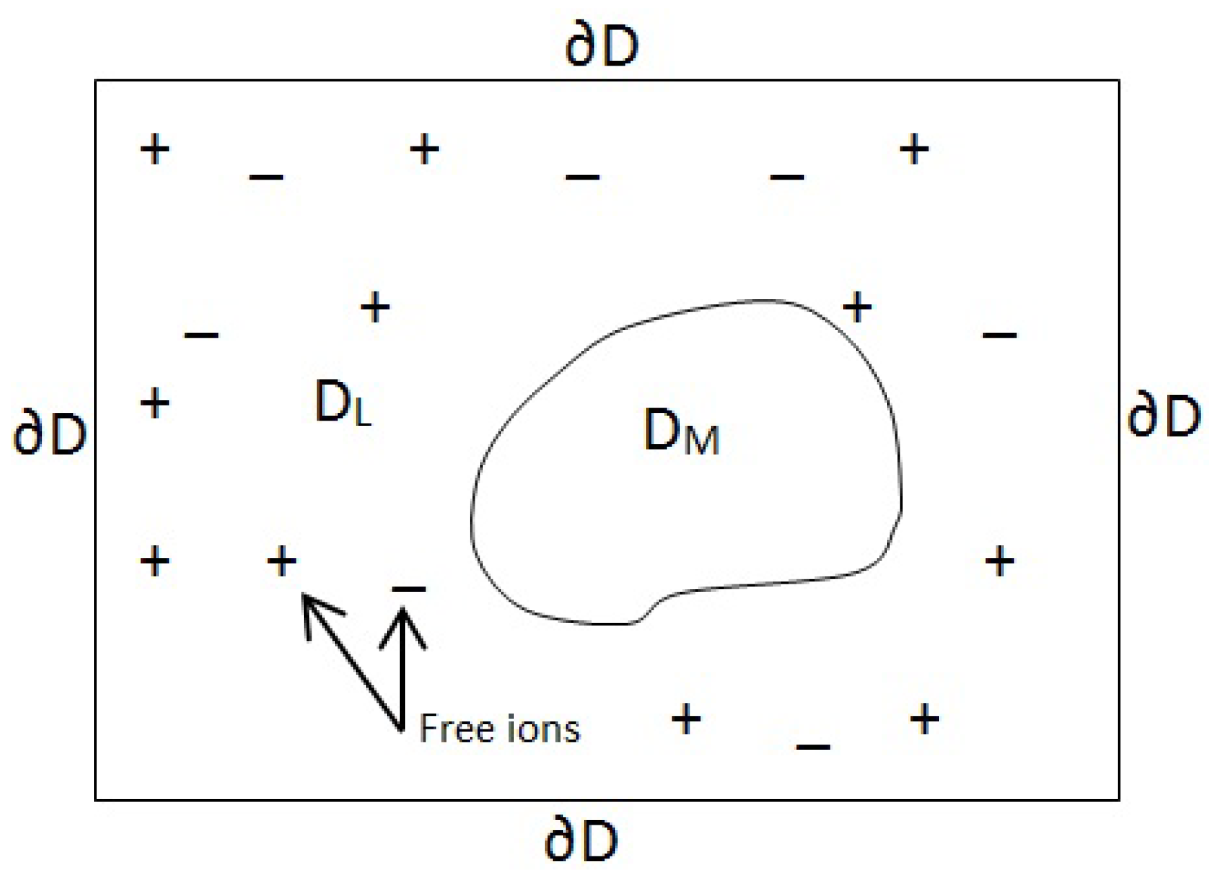
Figure 1. Schematic diagram of a biomolecular model in a domain D including two non-overlapping subdomains D L and D M , namely the liquid and molecule domains. + , denote positive and negative charge carriers.
Mathematics 11 02118 g001
Figure 2. The RBF-reference value from the approximation solution using the MQ function and 100 interpolation points.
Mathematics 11 02118 g002
Figure 3. The numerical solution for c = h n with RMSE = 0.0169.
Mathematics 11 02118 g003
Figure 4. The numerical solution for c = h n 2 with RMSE = 0.5389.
Mathematics 11 02118 g004
Figure 5. The numerical solution using the MQ function for c = d n with n = 40 and RMSE = 0.0013 .
Mathematics 11 02118 g005
Figure 6. Comparison of RMSE for various shape parameters using the MQ function with n = 40.
Mathematics 11 02118 g006
Figure 7. The numerical solution by using n = 50 , c = d n , with RMSE = 0.0079.
Mathematics 11 02118 g007
Figure 8. The numerical solution by using n = 70 , c = d n , with RMSE = 0.00027.
Mathematics 11 02118 g008
Figure 9. The numerical solution for the described model contains two molecules with c = d n , and RMSE = 0.0018 .
Mathematics 11 02118 g009
Figure 10. Comparison of RSMEs for various κ ( x ) with n = 70 .
Mathematics 11 02118 g010
Figure 11. Comparison of RMSEs for various D M with n = 70.
Mathematics 11 02118 g011
Figure 12. The numerical solution for the described model with five molecules contains c = d n and the RMSE = 0.0013 .
Mathematics 11 02118 g012
Table 1. Popular radial basis functions.
Name of FunctionAbbreviationDefinition
MultiquadricMQ φ ( r ) = c 2 + r 2
Inverse multiquadricIMQ φ ( r ) = 1 c 2 + r 2
Inverse quadraticIQ φ ( r ) = 1 c 2 + r 2
  GaussianGA φ ( r ) = exp ( c 2 r 2 )
  Polyharmonic splinePHS φ ( r ) = r 2 n 1 , n N , r 2 n ln r , n N
Thin plate splineTPS φ ( r ) = r 2 log r
Table 2. Results for various shape parameters using the MQ function with n = 40.
i Condition Number RMSE
11.1312  × 10 8 4.0  × 10 2
21.9033  × 10 7 3.7  × 10 3
31.0420  × 10 7 4.6  × 10 3
47.6998  × 10 6 5.1   × 10 3
56.4686   × 10 6 2.7   × 10 3
65.6856  × 10 6 3.2   × 10 3
75.1838  × 10 6 3.2  × 10 3
84.8844  × 10 6 3.7  × 10 3
94.6431  × 10 6 2.0  × 10 3
104.4586  × 10 6 2.0  × 10 3
c p = d n 3.0942  × 10 6 1.3  × 10 3
Table 3. Comparison of RSMEs using two different shape parameters and six different runs with n = 70.
RBF MQ RMSE IMQ RMSE IQ RMSE
c = d n        c = 0 . 815 d c = d n        c = 0 . 815 d c = d n        c = 0 . 815 d
run
16.0  × 10 4             5.6  × 10 3 7.9  × 10 4             4.9  × 10 3 6.0  × 10 3             1.2  × 10 3
22.1  × 10 4             9.6  × 10 3 5.3  × 10 4             2.1  × 10 3 3.2  × 10 3             6.7  × 10 4
33.4  × 10 4             8.9  × 10 3 8.4  × 10 4             4.3  × 10 3 5.9  × 10 3             5.2  × 10 4
45.7  × 10 4             6.0  × 10 3 7.5  × 10 4             3.7  × 10 3 5.1  × 10 3             7.3  × 10 4
53.7  × 10 4             7.8  × 10 3 4.5  × 10 4             5.0  × 10 3 2.7  × 10 3             3.8  × 10 3
65.5  × 10 4             3.4  × 10 3 7.4  × 10 4             2.2  × 10 3 8.6  × 10 3             1.4  × 10 3
Average4.2  × 10 4             6.4  × 10 3 6.8  × 10 4             3.7  × 10 3 5.2  × 10 3             1.3  × 10 3
Table 4. Comparison of RSMEs for various κ ( x ) with n = 70 .
RBF MQ RMSE IMQ RMSE IQ RMSE CSC RSME
κ ( x )
0.012.7  × 10 4 2.3  × 10 4 2.3  × 10 3 1.0  × 10 4
109.0  × 10 4 1.2  × 10 3 5.3  × 10 3 9.3  × 10 5
501.0  × 10 3 8.0  × 10 4 1.9  × 10 3 4.7  × 10 4
1001.1  × 10 3 4.7  × 10 4 1.4  × 10 3 9.6  × 10 5
Table 5. Comparison of RMSEs for various D M with n = 70.
RBF MQ RMSE IMQ RMSE IQ RMSE CSC RMSE
D M
12.7  × 10 4 1.0  × 10 3 8.2  × 10 4 4.5  × 10 4
27.5  × 10 4 3.6  × 10 4 3.7  × 10 3 9.2  × 10 5
51.3  × 10 4 3.7  × 10 4 4.3  × 10 3 8.8  × 10 5
Disclaimer/Publisher’s Note: The statements, opinions and data contained in all publications are solely those of the individual author(s) and contributor(s) and not of MDPI and/or the editor(s). MDPI and/or the editor(s) disclaim responsibility for any injury to people or property resulting from any ideas, methods, instructions or products referred to in the content.