Abstract
Under the global consensus of carbon peaking and carbon neutrality, new energy vehicles have gradually become mainstream, driven by the dual crises regarding the atmospheric environment and energy security. When choosing new energy vehicles, consumers prefer to browse the post-purchase reviews and star ratings of various new energy vehicles on platforms. However, it is easy for consumers to become lost in the high-star text reviews and mismatched reviews. To solve the above two issues, this study selected nine new energy vehicles and used a multi-attribute decision making method to rank the vehicles. We first designed adjustment rules based on star ratings and text reviews to cope with the issue of high star ratings but negative text reviews. Secondly, we classified consumers and recommended the optimal alternative for each type of consumer to deal with the issue of mismatched demands between review writers and viewers. Finally, this study compared the ranking results with the sales charts of the past year to verify the feasibility of the proposed method initially. The feasibility and stability of the proposed method were further verified through comparative and sensitivity analyses.
Keywords:
car services platform; new energy vehicles; multi-attribute decision making; star ratings; text reviews; consumer demands MSC:
90C70; 90B50
1. Introduction
With the development of urbanization and industrialization, fuel vehicles’ production and sales have been increasing yearly. Fuel vehicles have started entering millions of households, bringing convenience to people’s travel and affecting air quality [1]. It is well known that driving fuel vehicles will emit large amounts of exhaust gases, such as carbon dioxide gas and other compounds, which cause air pollution and global warming [2]. In addition, fuel vehicles are highly dependent on oil and other energy sources, and countries need to reserve or import oil and other energy sources, which is related to national energy security [3]. In contrast, new energy vehicles mainly use clean energy sources such as electricity and hydrogen, which are more friendly to the environment [2]. Therefore, driven by the dual crises regarding the atmospheric environment and energy security, new energy vehicles, represented by electric vehicles, came into being [4,5]. Under the global consensus of carbon peaking and carbon neutrality, governments encourage people to use new energy vehicles, which have gradually become mainstream [3].
Since the automobile is a highly involved and high-value product, consumers need to consider it carefully before purchasing a new energy vehicle [6]. When choosing a new energy vehicle, different consumers have different requirements. Some consumers focus on a desirable appearance, while others emphasize high performance. In addition, consumers often choose a new energy vehicle considering multiple factors that are sometimes conflicting. For example, compact vehicles are generally low in price but compact in space. By contrast, medium and large vehicles have better performance but may have a higher price. These complicate the selection process and consumers need to spend a great deal of time in decision making, which often lasts for months or even years [7]. As the Internet has developed, social media has begun to rise and hundreds of millions of users are posting comments on social media [8]. In China, auto forums such as Autohome and DCar are popular, where many consumers gather to exchange, discuss, and evaluate products, etc. Hence, there is a large amount of real user-generated content on auto forums [9]. When choosing a new energy vehicle, consumers prefer to browse the post-purchase reviews and star ratings of various new energy vehicles on platforms such as DCar. As more comments are viewed, consumers will have a better understanding of new energy vehicles, which will help them make the purchase decision. Thus, text reviews and star ratings on automotive forums are important to help consumers to assess the quality of products or services, reduce perceived risks and uncertainty, and then increase their purchase willingness [10,11].
However, a growing number of consumers are noticing that high-star ratings are far more numerous than low-star ratings. There are two main reasons for this. On the one hand, there is herd behavior when consumers give star ratings, which is easily influenced by average ratings or other consumers’ ratings [12]. On the other hand, a consumer who is dissatisfied with a product or service will give a negative text review along with a high star rating in order to avoid being harassed by the merchant [13]. However, consumers are still confused when reading a high star rating but a negative text review, and it is difficult for them to discern the reviewer’s true feelings about the products or services. In addition, with the development of social commerce, the number of text reviews has grown dramatically, and a wealth of reviews can reflect different consumers’ evaluations of products or services. Nevertheless, consumers often become lost in a large number of mismatched reviews. Consumer demands are diverse, and when the consumer and the reviewer have different demands, the reviewer’s comments may not be what the consumer wants. For example, some consumers are more concerned about performance when buying new energy vehicles, so they focus on power consumption, brakes, power, and other information when writing reviews. Others pursue appearance and focus on color, appearance, design, style, and other information when commenting. Meanwhile, some seek comfort, for family trips, and their reviews will mention family members’ feelings about the car, seats, and so on. Moreover, some of them are looking for experiential qualities, and their reviews will mention information about intelligent systems, services, etc. When performance-oriented consumers browse text reviews, they are likely to read reviews from appearance-oriented reviewers, comfort-oriented reviewers, and experience-oriented reviewers, which are not what they are looking for, and this type of consumer will easily become lost in the mass of mismatched reviews.
Therefore, this study proposed to address the following two issues.
- How to handle user-generated content with high star ratings but negative text reviews;
- How to identify different consumer demands and give targeted purchase suggestions.
Multi-attribute decision making refers to the ranking and selection of several alternatives by considering their performance under different attributes and using decision making methods. In research, linguistic term sets are used to denote the evaluation value of alternatives under different attributes. In 1965, Zadeh first defined the concept of fuzzy sets [14], and in 1975, Zadeh proposed the fuzzy linguistic approach to indicate linguistic information [15,16,17]. Subsequently, many linguistic term sets have been proposed one after another, including the hesitant fuzzy linguistic term set (HFLTS) [18], the interval-valued HFLTS [19], the hesitant 2-tuple fuzzy linguistic term set [20], and so on. In 2016, Pang added probability values to the hesitant fuzzy linguistic term sets and defined probabilistic linguistic term sets (PLTS) [21]. As mentioned above, consumers will consider various factors when purchasing a new energy vehicle, including space, power, power consumption, cost performance, interior, appearance, and comfort. Due to the conflict among factors, consumers often need to choose the best one among several new energy vehicles, and the selection process of new energy vehicles can be seen as a multi-attribute decision making problem, since text reviews are textual and consumers’ evaluations of a new energy vehicle are diverse in terms of certain attributes. Therefore, this research uses probabilistic linguistic term sets (PLTS) to transform text reviews into linguistic operators for subsequent decision analysis.
Based on the multi-attribute decision method, this study designed a mathematical model to select the optimal new energy vehicle. We evaluated the user-generated content on the DCar platform to test the proposed model and then used it to select an optimal new energy vehicle for consumers with different demands. The main contributions of this study are as follows. Firstly, this study has two types of data sources, namely star ratings and text reviews, which is different from previous studies that only consider a single data source. Moreover, adjustment rules are designed to modify the overrated high star ratings through the sentiments of the corresponding text comments. Secondly, this study uses the LDA model to identify consumer demands and proposes to select an optimal new energy vehicle for consumers with different demands. Thirdly, this study innovatively defines the concept of attribute richness and considers dual attribute characteristics, including richness and dissimilarity, to calculate attribute weights. This is different from previous studies that only use the entropy weight method or TF-IDF value to calculate attribute weights. Fourthly, this research conducts a cross-sensitivity analysis for two pairs of parameters, namely the star rating–text reviews parameter and the dissimilarity–richness parameter.
The remainder of this manuscript is organized as follows. Section 2 is the literature review. Section 3 is the research methodology. This study defines the aggregation method for star ratings and text reviews. Moreover, this research defines the concept of attribute richness and designs the weight calculation method and mathematical model. Section 4 presents a case study of new energy vehicle selection on DCar. Comparison analysis and sensitivity analysis are conducted in Section 5. Finally, Section 6 offers the conclusions.
2. Literature Review
2.1. New Energy Vehicles
Many studies try to identify the influencing factors that cause consumers to buy new energy vehicles. Wang and Dong surveyed consumers in four Chinese cities, Beijing, Shanghai, Tianjin, and Chongqing, and found that perceived ease of use, subjective norms, and perceived behavioral control all significantly increased consumer purchase intention, and perceived behavioral control had a significant moderating effect on subjective norms [22]. Interestingly, this study also found that perceived ease of use had a significant impact on those who would be unwilling to purchase a new energy vehicle, while subjective norms had a significant influence on potential consumers who were hesitant to purchase a new energy vehicle [22]. Ma et al. found that, on the one hand, the subsidy policy and tax reduction policy can stimulate consumers to buy new energy vehicles by reducing their purchase and use costs, and the tax reduction policy has the strongest long-term effect [23]. On the other hand, China’s purchase restriction policy and traffic restriction policy on fuel vehicles can improve consumers’ willingness to purchase new energy vehicles by regulating supply and demand in the market [23]. Significantly, it is also found that green self-identity has a significant positive effect on both personal norms and the purchase willingness regarding new energy vehicles, and the mianzi and green peer impact can positively regulate the relationship between green self-identity and purchase willingness [24]. In addition to psychological factors, subsidy policies, environmental awareness, etc., product performance also affects consumers’ purchase willingness regarding new energy vehicles. Research found that product attributes such as price, charging time, driving distance, pollutant emission, and energy consumption cost significantly affect consumer purchase intention [25].
Along with the development of social media, many studies have been conducted to analyze user-generated contents, such as star ratings and text reviews, but there are fewer studies on new energy vehicles. Cai et al. first extracted product features from new energy vehicle reviews by using machine learning models, and then used hierarchical clustering models for feature classification, followed by demand ranking based on customer satisfaction scores, and finally employed statistical methods for demand preference identification [26]. Since 2017, some studies have started to extend the multi-attribute decision making method to the new energy vehicles field. Liu et al. first established a capability–willingness–risk (C-W-R) evaluation indicator system and then proposed a multi-criteria decision making method based on the best–worst method, prospect theory, and VIKOR method to obtain the best innovative supplier for new energy vehicle manufacturers [27]. Nicolalde et al. firstly used the removal effect of a criterion method to weight the criteria; used the VIKOR, COPRAS, and TOPSIS methods to evaluate the 20 materials, and obtained the best phase change material, which was the savENRG PCM-HS22P [28]. However, these studies mainly focus on the selection of new energy vehicle suppliers, the selection of vehicle materials, and the locations of charging stations and so on. There is still a lack of research on new energy vehicle brand selection based on user-generated content.
2.2. Multi-Attribute Decision Making Method
The multi-attribute decision making method generally involves several attributes and several solutions, and the optimal alternative is selected by fusing the experience and wisdom of several experts [29,30,31]. The evaluation value of each alternative under different attributes is given by each expert, which is denoted by various linguistic term sets. Common linguistic term sets include intuitionistic fuzzy sets [32], probabilistic linguistic term sets [33], interval values [34], linguistic distribution assessments [35], and so on. There are abundant decision making methods in the field of multi-attribute decision making, such as TOPSIS [36], TODIM [37], VIKOR [38], ELECTRE [39], MULTIMOORA [40], and so on. Multi-attribute decision making methods were extended to various fields, including distribution center site selection [41], the selection of emergency solutions [42], the selection of disaster handling solutions [43], and so on. Wang et al. used the fuzzy AHP method and fuzzy deviation maximizing method to calculate attribute weights and combined five types of multi-attribute decision methods, namely the TOPSIS, TODIM, VIKOR, PROMETHEE, and ELECTRE methods, with the simple dominance principle to rank the bidding options and select the best one [44]. Dabous et al. established a utility function set based on the analytic hierarchy process and multi-attribute utility functions for large pavement network selection considering the sustainability of pavement sections [45]. Yang et al. constructed an evaluation index system for the coordinated development of regional ecology based on ecological, economic, social, and policy factors; used the closeness to construct the value function to calculate attribute weights, and finally evaluated the regional ecological development performance of 27 cities in China based on the proposed heterogeneous decision model [46]. Huang et al. used interval numbers to represent the attribute information in the group decision matrix, and then proposed a distributed interval weighted average operator to integrate qualitative data and quantitative judgments; then, they defined relevant operation rules, and finally ranked and selected the best green suppliers [34]. To solve the problem that different approximation methods for rough sets affect the results, Wang et al. first proposed an attribute metric method based on fuzzy sets, and then constructed Choquet integral operators based on the attribute metric and matching degree, and finally used the operators to rank and select the alternatives [47].
2.3. Product Ranking Method Based on Multi-Attribute Decision Making
Fan et al. divided the text-review-based product ranking process into three phases, namely product feature extraction, sentiment analysis, and product ranking, and pointed out that information fusion methods could be used to integrate the sentiment analysis results [48]. Common information fusion methods include the WA operator, OWA operator, fusion operator based on intuitionistic fuzzy numbers, fusion methods based on weighted directed graph construction, and information fusion methods based on hesitant fuzzy numbers [48]. Most of the mentioned information fusion methods belong to the field of multi-attribute decision making, and product ranking based on multi-attribute decision methods has indeed attracted the attention of many scholars. A brief description of some recent studies is shown in Table 1.

Table 1.
Recent studies on product ranking based on multi-attribute decision making methods.
According to Table 1, in terms of data sources, most papers only used text reviews for product ranking, and a few papers only used star ratings [49,52]. It is worth noting that some of the papers’ data sources included text reviews and star ratings. However, they did not integrate these two types of data sources; instead, they used text reviews and star ratings separately. Qin et al. used star rating data to mark the polarity of reviews (positive, neutral, negative), and sentiment analysis and product ranking were only based on text reviews [59]. Bi et al. assessed price, location, overall ratings, and text reviews; calculated the prospect values for each of these four types of data, and selected the optimal hotels based on the prospect value [60]. Tayal et al. built a benchmark to evaluate the performance of ranking methods based on attribute ratings, and the product ranking method was only based on reviews [61]. In terms of applications, many studies focused on hotels, automobiles, and mobile phones. For the contribution phases, data processing, sentiment analysis, weight calculation, and product ranking all have been innovatively studied.
3. Methodology
This study proposes a new mathematical model for new energy vehicle selection based on two types of data, which are text reviews and star ratings, considering the dual characteristics of attributes. In Appendix A, Table A1 lists all acronyms used in this paper.
3.1. Preliminaries
In this section, we review the definition of probabilistic linguistic term sets, the score of PLTS calculation formula, the comparison rule of PLTS, and the distance measure formula.
Definition 1
([21]). Let be a linguistic term set (LTS) with asymmetric subscripts. Based on LTSs, probabilistic linguistic term sets (PLTSs) consider probability values for different linguistic terms. Thus, a PLTS can be defined as
where refers to the k-th linguistic term with the probability value . As the elements in , the linguistic terms are arranged in ascending order and denotes the number of elements in . The probability value must be greater than or equal to 0, and the sum of all probability values of a PLTS must be less than or equal to 1. When the sum of the probability values is less than 1, the evaluation information is incomplete. Then, it requires normalization to make the sum of the probability values equal to 1. The normalized probability value is , where .
Definition 2
([21]). Given a PLTS , the score of , also called the expected value, can be calculated as
where denotes the number of elements in , is the subscript of the linguistic term , and is the probability value of the linguistic term . The deviation degree of is defined as
For any two PLTSs, and , the comparison rules are defined as follows:
- (1)
- If , then ;
- (2)
- If , then ;
- (3)
- When , if , then ; if , then ; if , then .
Definition 3
([21]). For any two PLTSs, and , if , then requires the use of additional linguistic terms with probability values of 0 until . If , then requires the use of additional linguistic terms with probability values of 0 until . If , then the distance between these two PLTSs can be calculated as
where and denote the subscripts of linguistic terms and , respectively. Meanwhile, and denote the probability values of linguistic terms and , respectively.
3.2. Problem Description
In this study, the selection of new energy vehicles is considered as a multi-attribute decision problem, and a new method is proposed to select an optimal new energy vehicle from several new energy vehicles. Suppose that there are n new energy vehicles, also called alternatives, and m attributes of new energy vehicles. Let be an alternative set and let be an attribute set. The weights of these attributes are denoted by , where . In addition, in the first stage, this study used the LDA model to classify the reviews under each alternative into topics. Thus, let be a topic set, where denotes the total number of topics. Notably, this study will distinguish whether it is based on star ratings or text reviews through a symbol in the right superscript. The symbol “sr” in the right superscript denotes star ratings, while “tr” refers to text reviews.
Let a seven-level LTS denote the evaluation values obtained by text reviews. Probabilistic linguistic evaluation values for vehicle with respect to attribute and the topic are provided by consumers, where ; ; . Probabilistic linguistic evaluation values with the probability are included in the PLTS , where , and . Then, the sub-topic text review decision matrices and the text review decision matrix are obtained.
Consumers on DCar can rate the attributes of new energy vehicles on a scale of 1 to 5. Therefore, let a five-level LTS denote attribute ratings. Probabilistic linguistic evaluation values with the probability are included in the PLTS , where , and . Then, the sub-topic star rating decision matrices and the star rating decision matrix are obtained.
3.3. Mathematical Model
The proposed methodology consists of four stages, as shown in Figure 1. The first stage is the formation of the star rating decision matrix and the text review decision matrix . The second stage is the formation of the comprehensive decision matrix . The third stage is weight calculation. The fourth stage is alternative ranking and selection.
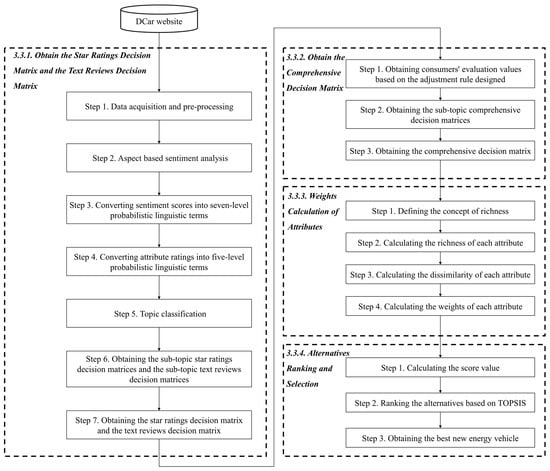
Figure 1.
The proposed method for the product ranking problem.
3.3.1. Obtain the Star Rating Decision Matrix and the Text Review Decision Matrix
Step 1. Data acquisition and pre-processing.
User-generated data on automotive forums generally include text comments and star ratings of attributes. We use the Octopus collector to obtain online comments and star ratings from relevant automotive forums and then carry out data pre-processing. First of all, we carry out data cleaning, removing incomplete data and duplicate data. Secondly, we use the Jieba library to segment text reviews and remove useless words, stop words, punctuation marks, etc. Thirdly, we perform the POS tagging. Fourthly, we extract key new energy vehicle attributes based on TF-IDF values.
Step 2. Aspect-based sentiment analysis.
We compare the attributes extracted based on reviews with those in star ratings and determine the attribute set mainly based on the latter. Then, we use the pysenti library to conduct the dictionary-based sentiment analysis. Firstly, we build several pairs of attribute–sentiment words as a seed table. Secondly, we search the attributes of the seed table in the dataset and obtain words or phrases associated with each attribute. Thirdly, we identify the sentiment polarity (positive, neutral, negative) of each word or phrase according to the sentiment dictionary. Fourthly, we assign weights to the sentiment polarity of multiple sentiment words under each attribute in combination with the sentence structure, and then the weighted sum method is used to obtain the sentiment polarity score for each attribute.
Step 3. Convert sentiment scores into seven-level probabilistic linguistic terms.
Based on the equidistant binning method, the sentiment scores of the attributes are divided into seven segments equidistantly and then converted into the corresponding seven-level probabilistic linguistic terms.
Step 4. Convert attribute ratings into five-level probabilistic linguistic terms.
The attribute ratings were obtained in Step 1, ranging from 1 to 5, and thus can be directly converted into five-level probabilistic linguistic terms. Specifically, five ratings, namely excellent, good, average, bad, and terrible, can be replaced by the linguistic terms , , , , and .
Step 5. Topic classification.
Text reviews are often one-sided and the formation process will be influenced by consumer demands. For example, consumers who pursue appearance will also focus on the description of appearance when commenting. In order to match the demands of comment writers and comment viewers, it is necessary to firstly identify the diverse demands of consumers. This study used the LDA model to classify consumers. The LDA model is used to classify all the comments after pre-processing into topics and the optimal number of topics is selected on the basis of perplexity. It is worth noting that the number of topics under each alternative is the same, but the percentage of each topic may be different.
Step 6. Obtain the sub-topic star rating decision matrices and the sub-topic text review decision matrices.
We calculate the proportion of each linguistic term for each alternative under different sub-topics and attributes, and thus form the sub-topic text review decision matrices and the sub-topic star rating decision matrices .
Step 7. Obtain the star rating decision matrix and the text review decision matrix.
The sub-topic decision matrices under each alternative are averaged separately and integrated into a comprehensive decision matrix . The aggregation formula is as follows.
where denotes the number of topics and is the probability value of the k-th linguistic term for alternative under the attribute and the topic . Notably, for sub-topic decision matrixes of text reviews, , while, for sub-topic decision matrixes of star ratings, . Finally, normalization processing is as follows.
3.3.2. Obtain the Comprehensive Decision Matrix
Since 1974, many studies have revealed that the human thinking process is influenced by “two systems”, which are System 1 and System 2 [62,63]. System 1 is biased fast thinking, while System 2 is rational slow thinking. Specifically, System 1 is intuitive, automatic, and associative, operating unconsciously and quickly, without much mental effort [62,63]. In contrast, System 2 requires a lot of mental effort and concentration and is controlled, disciplined, and focused on the outcome of the decision [62,63].
When consumers evaluate products, they are often first required to rate the product attributes and are further asked to make a comment. The assignment of star ratings involves fast thinking, related to intuition, association, experience, and other thinking in System 1. Thus, star ratings are likely to be vague and biased and do not accurately reflect consumers’ evaluations of products or services. Cho et al. argued that herd behavior is probably occurring when consumers give star ratings because they can see the average star rating, which may influence their own rating values [64]. Some experiments have also shown that consumers tend to modify their own rating values after seeing the ratings given by others, with 70% of the final star ratings derived from their own initial estimates and 30% from others’ estimates [64]. Considering the fuzziness and bias of star ratings, many consumers are skeptical of high star ratings. Gavilan et al. found that web users prefer to trust low-value ratings rather than high-value ratings and that consumers’ trust in high ratings depends on the number of reviews [65]. Hong et al. mentioned that consumers do not believe in high star ratings unless the review content is also positive [66]. Cho et al. argued that the positive sentiment of text reviews would compensate for consumers’ tendency to discount high star ratings, but the negative sentiment of text reviews would aggravate consumers’ suspicion of high ratings [64]. Based on the above analysis, we cannot rank products only based on star ratings because star rating values cannot accurately reflect consumers’ evaluations of products.
The formation of text comments involves rational, slow thinking, related to the controlled, thoughtful, logical, and other thinking in System 2. When composing text reviews, consumers spend time thinking, forming words, and then logically writing them down. However, writing reviews is burdensome for consumers, not providing intuitive benefits but taking up time. Therefore, consumers are reluctant to spend a lot of effort in reviewing. Text reviews are generally not too long, and the content of comments is one-sided, but they can be used as a supplement to star ratings. It has also been shown that text reviews have additional information that significantly influences product demand [64].
Based on the above analysis, this study is mainly based on star ratings, complemented by text reviews, to obtain consumers’ evaluation values of products. Specifically, this study argues that star ratings are often overestimated and adjusts star ratings with the sentiment scores of text comments. This study argues that there are four states of linguistic terms, as shown in Figure 2. Firstly, this study excludes the case of low-star but positive text reviews, which is also rare. Secondly, linguistic terms are acceptable in the case of high-star and positive text reviews or low-star and negative text reviews, which do not require adjustment. Finally, those linguistic terms for high-star but negative text reviews need to be adjusted. In other words, when the text content of the high star rating is negative, the high star rating needs to be down-adjusted. The adjustment rules are shown in Table 2.
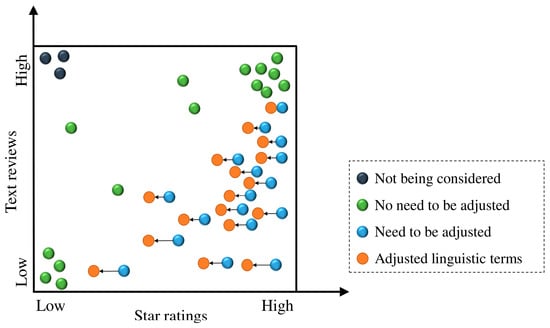
Figure 2.
Four states of linguistic terms.
Table 2.
The designed adjustment rules.
In Table 2, the first column on the left is the probabilistic linguistic terms of star ratings, the first row above is the probabilistic linguistic terms for the sentiment scores of the text reviews, and the rest are adjusted probabilistic linguistic terms. The general rule is to adjust the star ratings through the sentiments of corresponding text reviews. This study only considers the situation of high-star and negative text reviews, and ignores the situation of low-star and positive text comments. Thus, the adjustment direction is downward, and the adjustment range is [0,1], with the same unit adjustment for each row. When the difference between the star rating and the sentiment of the text comment is larger, the adjustment of the star rating is larger; otherwise, the adjustment is smaller or even zero. For example, when the star rating is , the probabilistic linguistic terms for the sentiment scores of text comments might be . Meanwhile, when the review is , the high star rating is acceptable, and adjustment is not required. However, when the review is , , , , , or , the star rating may be overrated and needs to be modified with increasing amounts of adjustment. Similarly, when the probabilistic linguistic term of the review is greater than or equal to , the star rating is credible. However, if the review is , the star rating is to be adjusted to . Meanwhile, if the review is , , , the star rating is to be adjusted to , , , respectively. Notably, this study does not consider situations where star ratings are underrated. Thus, when the star rating is , the rating value will not be adjusted upward, even if the comment is positive.
Steps to obtain the comprehensive decision matrix are as follows.
Input. Step 3, step 4, and step 5 in Section 3.3.1.
Step 1. Obtain consumers’ evaluation values.
Based on the adjustment rule designed in this study, the probabilistic linguistic terms of the star ratings are adjusted and the final consumer evaluation values are obtained.
Step 2. Obtain the sub-topic comprehensive decision matrices.
Calculate the proportion of each linguistic term for each alternative under different sub-topics and attributes, and thus form the sub-topic comprehensive decision matrices.
Step 3. Obtain the comprehensive decision matrix.
The average of the sub-topics’ decision matrices under each alternative is separately calculated using Equation (5), and then normalized by using Equation (6) and integrated into a comprehensive decision matrix.
Output. A comprehensive probabilistic linguistic decision matrix.
3.3.3. Weight Calculation of Attributes
This study first defined the concept of attribute richness and then calculated the weights based on richness and dissimilarity. Since this study contained dual data sources, the richness (RI) and dissimilarity (DI) were calculated based on the star rating decision matrix and the text review decision matrix, respectively. Next, the symbol ‘ri’ will be used to refer to richness, ‘di’ to refer to dissimilarity, and ‘sr’ to denote star ratings and ‘tr’ to denote text reviews.
- (1)
- Calculating the richness of attributes
When the distribution of the evaluation value of an attribute is concentrated, it means that many customers have the same evaluation of this attribute, which contains less information. Therefore, this attribute weight should be decreased. On the contrary, when the distribution of the evaluation value of an attribute is balanced, it means that consumers have a rich and diverse evaluation of the attribute, which can provide more information. In this case, this attribute has a higher richness degree. Thus, this attribute weight should be increased.
The following two probabilistic linguistic term sets are used to illustrate attribute richness.
- Let a PLTS express the consumers’ evaluation value of attribute 1. It shows that 60% of consumers believe that attribute 1 is average, 23% claim that it is good, and fewer consumers believe that attribute 1 is bad, very good, or excellent.
- Let a PLTS express the consumers’ evaluation value of attribute 2. It shows that 27% of consumers believe that attribute 2 is bad, and 23% claim that it is good. Moreover, 20%, 14%, and 16% of consumers separately believe that attribute 2 is average, very good, and excellent.
Among the two attributes above, the consumers’ evaluation of attribute 1 focuses on average and good, while the consumers’ evaluation of attribute 2 is diverse, the probability values of different linguistic terms are closer, and the evaluation value for attribute 2 contains richer information. Attribute 2 should be assigned a larger weight because different consumers have rich and diverse feelings about attribute 2, which brings a greater influence on the selection of products.
Definition 4.
Let be a probabilistic linguistic term set, . Let be the ideal equilibrium PLTS of , and . The distance measure between and can be defined as follows:
where denotes the subscript of linguistic term , and denotes the probability value of linguistic term . is the number of linguistic terms in or . Meanwhile, is a fixed value, referring to the probability value for all linguistic terms in and .
This study calculates the attribute richness by calculating the distance between the evaluation value and its ideal equilibrium evaluation value. The steps to calculate the richness are as follows.
Step 1. Calculate the distance between the evaluation value of alternative under attribute and its ideal equilibrium evaluation value according to Equation (7) (based on the star rating decision matrix).
Step 2. Calculate the average distance between attribute and the ideal equilibrium evaluation value (based on the star rating decision matrix).
Step 3. Calculate the richness (based on the star rating decision matrix).
The smaller the average distance between the evaluation value and the ideal equilibrium solution, the higher the richness and the greater the weight.
Step 4. Calculate the distance between the evaluation value of alternative under attribute and its ideal equilibrium evaluation value according to Equation (7) (based on the text review decision matrix).
Step 5. Calculate the average distance between attribute and the ideal equilibrium evaluation value (based on the text review decision matrix).
Step 6. Calculate the richness (based on the text review decision matrix).
The smaller the distance between the evaluation value and the ideal equilibrium solution, the higher the richness and the greater the weight.
Step 7. Calculate the comprehensive richness (based on the star rating decision matrix and the text review decision matrix).
where and are a pair of parameters that represent the ratio of star ratings to text reviews and .
- (2)
- Calculating the dissimilarity of attributes
When the distance between the evaluation values under two attributes is larger, the similarity between these two attributes is lower and the dissimilarity is higher. Based on the clustering theory, when the average distance between an attribute and other attributes is larger, the attribute will have a greater effect on the results, and this attribute should be assigned a larger weight. Otherwise, it should be assigned less weight. The steps for calculating the dissimilarity are as follows.
Step 1. Calculate the distance between the evaluation values of attribute and attribute under alternative according to Equation (4) (based on the star rating decision matrix).
Step 2. Calculate the average distance between attribute and attribute (based on the star rating decision matrix).
Step 3. Calculate the dissimilarity (based on the star rating decision matrix).
Step 4. Obtain the normalized dissimilarity (based on the star rating decision matrix).
Step 5. Calculate the distance between the evaluation values of attribute and attribute under alternative according to Equation (4) (based on the text review decision matrix).
Step 6. Calculate the average distance between attribute and attribute (based on the text review decision matrix).
Step 7. Calculate the dissimilarity (based on the text review decision matrix).
Step 8. Obtain the normalized dissimilarity (based on the text review decision matrix).
Step 9. Calculate the comprehensive dissimilarity (based on the star rating decision matrix and the text review decision matrix).
where and are a pair of parameters that are the same as the parameters in Equation (12) and .
As we obtained the richness and dissimilarity of each attribute in the previous part, the attribute weights based on richness and dissimilarity can be calculated as follows.
where and are a pair of parameters that represent the ratio of richness to dissimilarity and . When the richness of an attribute is larger and the dissimilarity is greater, the weight of this attribute is greater.
3.3.4. Alternative Ranking and Selection
Since this study integrates the star rating decision matrix and the text review decision matrix into a comprehensive decision matrix with 15 linguistic terms, we choose the TOPSIS method [67], which is easier to perform, for the ranking and selection of the best alternative with the following steps.
Step 1. Calculate the score value of alternative under attribute .
Step 2. Obtain the normalized score value .
Step 3. Obtain the weighted score value .
Step 4. Calculate the maximum and minimum values.
Let be the set of maximum values, where , and let be the set of minimum values, where .
Step 5. Calculate the distance and from the ideal positive solution and from the ideal negative solution, respectively.
Step 6. Calculate the nearness degree of alternative .
Rank the alternatives in descending order of nearness degree, and the one with the greatest nearness degree is the optimal alternative.
4. Case Study: New Energy Vehicle Selection in DCar.com
DCar.com is a car information and service platform that categorizes cars into new energy cars, SUVs, sports cars, and other types, providing information on cars including price, parameter configuration, size, sales, word of mouth, and more. In the Word-of-Mouth section, numerous car buyers rate the attributes of cars that they have purchased on a scale of 1 to 5, and then upload pictures of the car and post reviews of their experiences with the car. Users of the DCar website can browse through the attribute ratings and reviews of cars to obtain information about the cars and make better purchasing decisions. Therefore, ranking cars based on attribute ratings and text reviews on DCar.com is a worthy concern.
4.1. Data Source and Data Processing
Based on the sales rankings of new energy vehicles on DCar.com for the past year, and taking into account the diversity of brands and sizes of vehicles, this study selected the top five compact new energy vehicles (CNEV) in terms of sales, namely car A, car B, car C, car D, and car E, denoted hereafter by , , , , and . Moreover, the top four medium and large new energy vehicles (MLNEV) in terms of sales were also selected, namely car F, car G, car H, and car I, and these vehicles are denoted hereafter by , , , and . This study obtained star ratings and text reviews for the above nine cars on DCar.com and the number of ratings/reviews for each vehicle is shown in Table 3.
Table 3.
Top 9 new energy vehicles and their corresponding number of ratings/reviews.
When purchasing cars, consumers may have different demands, which will be further reflected in their own attribute ratings and text reviews. In order to avoid averaging consumer opinions, this study first classified consumers and then constructed decision matrices for different consumer types under each vehicle. Specifically, after pre-processing the text reviews, this study used the LDA algorithm to classify consumers for compact and medium–large vehicles, respectively. This study first determined topic numbers based on the perplexity metric, and then artificially named consumer types through topic high-frequency words, as shown in Table 4. Finally, there are three types of consumers for CNEV, namely family-oriented consumers, appearance-oriented consumers, and professional-oriented consumers. The three consumer types are expressed as , , and . Moreover, there are four types of consumers for MLNEV, namely experiential-oriented consumers, appearance-oriented consumers, professional-oriented consumers, and performance-oriented consumers. The four consumer types are expressed as , , , and . Table 5 and Table 6 show the number of ratings/reviews corresponding to the different consumer types for each vehicle.
Table 4.
Consumer demands and their corresponding high-frequency words.
Table 5.
The number of ratings/reviews under different consumer types for CNEVs.
Table 6.
The number of ratings/reviews under different consumer types for MLNEVs.
In terms of star rating processing, this study obtained attribute ratings for the above nine cars on DCar.com, where the attributes include space, power, handling, power consumption, comfort, appearance, interior, and cost performance, and these attributes are denoted hereafter by , , , , , , , and . Attributes are rated on a scale of 1 to 5, indicating terrible, bad, average, good, and excellent. This list is replaced hereafter by the linguistic terms , , , , and . In terms of text review processing, this study divided the sentiment scores of text reviews into seven levels, namely terrible, very bad, bad, average, good, very good, and excellent. This list is replaced hereafter by the linguistic terms , , , , , , and . Finally, the overall star rating decision matrix and the text review decision matrix were obtained according to steps 1 to 7 in Section 3.3.1, as shown in Table A2, Table A3, Table A4, Table A5, Table A6, Table A7, Table A8 and Table A9.
4.2. Obtaining the Comprehensive Decision Matrix
This study argues that star ratings are often overestimated and thus designs adjustment rules. The adjustment direction can only be downwards. When the text content of a high star rating is negative, the high star rating needs to be adjusted downwards. According to steps 1 to 3 in Section 3.3.2, this study obtained the comprehensive probabilistic linguistic decision matrix shown in Table 7, Table 8, Table 9, Table 10, Table 11, Table 12, Table 13, Table 14 and Table 15.
Table 7.
The comprehensive probabilistic linguistic decision matrix (alternative 1).
Table 8.
The comprehensive probabilistic linguistic decision matrix (alternative 2).
Table 9.
The comprehensive probabilistic linguistic decision matrix (alternative 3).
Table 10.
The comprehensive probabilistic linguistic decision matrix (alternative 4).
Table 11.
The comprehensive probabilistic linguistic decision matrix (alternative 5).
Table 12.
The comprehensive probabilistic linguistic decision matrix (alternative 6).
Table 13.
The comprehensive probabilistic linguistic decision matrix (alternative 7).
Table 14.
The comprehensive probabilistic linguistic decision matrix (alternative 8).
Table 15.
The comprehensive probabilistic linguistic decision matrix (alternative 9).
4.3. Calculating the Weights of Attributes
This study divided new energy vehicles into two categories, compact (CNEV) and medium–large (MLNEV), and argued that consumers have different priorities for these two types of vehicle attributes. For example, consumer demand for space should be lower for compact than for medium–large vehicles, because compact vehicles are inherently small in space. Therefore, this study calculated attribute weights for compact new energy vehicles (including ) and medium–large new energy vehicles (including ) separately.
This study introduced the concept of attribute richness and calculated attribute weights based on richness and existing dissimilarity. Since this study used two data sources, star ratings and text reviews, the richness and dissimilarity were calculated based on the star rating comprehensive decision matrix and the text review comprehensive decision matrix, respectively. The richness and dissimilarity of each attribute were obtained according to the steps in Section 3.3.3 and are shown in Table 16.
Table 16.
The richness and dissimilarity of each attribute.
In order to calculate the attribute weights, this study needs to determine the parameters (). Existing research supports that there is herding behavior when consumers give star ratings, which is easily influenced by others’ star ratings and the average star rating. This leads to star ratings commonly being overestimated and untruthful, while text reviews are more trustworthy. Consequently, this study let the star rating parameter be 0.4 and the text review parameter be 0.6. Moreover, we let the richness parameter be 0.5 and the dissimilarity parameter be 0.5. Table 17 shows the attribute weights for compact and medium–large new energy vehicles.
Table 17.
The attribute weights for compact and medium–large new energy vehicles.
According to the prioritizations between the attributes in Table 18, for compact new energy vehicles, consumers place an emphasis on comfort, interior, and appearance, while, for medium and large new energy vehicles, consumers value power consumption, space, and handling. Moreover, for compact and medium–large new energy vehicles, power and cost performance are given the least attention.
Table 18.
Prioritizations between the attributes.
4.4. Results and New Energy Vehicle Recommendations
Based on the TOPSIS method, the nearness degree of each alternative was calculated according to the steps in Section 3.3.4. Ranking the alternatives based on the nearness degree, from largest to smallest, this study obtained the ranking results shown in Table 19. This is the same as the sales ranking in the past year, proving the feasibility of the proposed method. Car A is recommended when consumers want to purchase a compact new energy vehicle, and car F is recommended when purchasing a medium or large new energy vehicle.
Table 19.
The ranking results.
This study divided consumers who buy compact new energy vehicles into three categories and those who buy medium and large vehicles into four categories. Different types of consumers have different consumer needs, and each new energy vehicle has different superior and inferior attributes. It is not reasonable to recommend new energy vehicles without considering the heterogeneity of consumer needs. Therefore, based on the previous consumer classification, this study intends to recommend new energy vehicles for different consumer demands. We input the sub-topic comprehensive decision matrices obtained in step 2 of Section 3.3.2 and re-rank the alternatives based on the steps in Section 3.3.4. The results are shown in Table 20. In terms of CNEV, for family-oriented consumers, car B and car E are recommended. Meanwhile, for appearance-oriented consumers, car A and car B are favored. Next, for professional-oriented consumers, car A and car D are preferred. In terms of MLNEV, for family-oriented consumers, car H and car F are recommended. For other types of consumers, car F and car G are favored.
Table 20.
The ranking results for different consumer demands.
5. Comparative and Sensitivity Analysis
5.1. Comparative Analysis
This study proposes a new mathematical method to rank new energy vehicles. The results are consistent with the sales ranking of new energy vehicles on DCar.com in the past year, which initially verifies the feasibility of the proposed method. To further test the effectiveness of our method, this section will describe comparative analyses in three aspects: multi-attribute decision making method, weight, and data source.
In terms of multi-attribute decision making methods, this study designs adjustment rules based on the star rating decision matrix and the text review decision matrix. The adjusted comprehensive decision matrix contains at most 15 elements in probabilistic linguistic term sets, which greatly increases the difficulty of ranking the alternatives. This study ranks the alternatives using the TOPSIS method in the case study, and the best options are car A and car F. TODIM, PROMETHEE, and VIKOR are common multi-attribute decision making methods but are more complex to compute and unsuitable for probabilistic linguistic term sets with too many elements. However, the score function is a simpler method for ranking alternatives. We assigned the same weights to the attributes as in Section 4.3, first calculating each attribute’s score values separately, and then calculating the weighted score values for each alternative. The results are shown in Table 21. It is clear that the score function and the TOPSIS method have the same calculation results.
Table 21.
The results based on score function method.
In terms of weighting, the term frequency-inverse document frequency (TF-IDF) is often used to determine the weight of each attribute [68,69]. This study obtained the TF-IDF values of the attributes in step 1 of Section 3.3.1 and normalized the TF-IDF values to obtain the attribute weights as shown in Table 22. Moreover, this study used the TOPSIS method to calculate the nearness degree of the alternatives and obtained ranking results of and . The optimal compact new energy vehicle (CNEV) is car A and the optimal medium and large vehicle is car F, which is the same as the optimal solutions obtained in this study. However, alternative 2 was ranked last among the CNEVs, and the rankings of alternative 8 and alternative 9 among the MLNEVs were reversed. This illustrates the limitations in calculating weights only based on TF-IDF values.
Table 22.
The attribute weights based on the TF-IDF values.
In terms of data sources, this study argued that star ratings are often overestimated and text reviews are one-sided. Thus, we integrated these two types of data sources. However, most papers only used text reviews for product ranking [53,54,55,70], and a few papers only used star ratings [49,52]. As shown in Table 23, TR indicates alternative selection only based on the text review decision matrix and SR indicates alternative selection only based on the star rating decision matrix. Three multi-attribute decision methods were used, namely the TOPSIS, Dempster–Shafer evidence theory (DSET), and TODIM methods.
Table 23.
Ranking results based on different methods.
Comparing methods 1–5 with the method proposed in this study, it was found that there were significant limitations when ranking the options only based on text reviews, with large deviations in the ranking results. The recommended compact cars were alternatives 4 and 5, which should have been ranked lower. The recommended mid-size cars were option 6 and option 9. Instead, it is more credible to rank the alternatives only based on star ratings. The best compact car is alternative 1, and that for medium and large cars is alternative 6, which is similar to the results obtained in this study. However, there is a reversal in the ranking of some alternatives, such as alternative 4 and alternative 5, and alternative 7 and alternative 8. The possible reasons for this are as follows. A consumer first gives a star rating and then writes a complementary text review. Thus, the content in the text reviews is related to the star rating level. When the star rating is high, the consumer tends to add unsatisfactory aspects to the text review. When the star rating is low, the consumer may add satisfactory remarks to the text review or make a mild complaint in order to avoid harassment from the merchant. Consequently, text reviews for lower star ratings are likely to be mildly positive, while text reviews for higher star ratings are likely to be mildly negative. In this case, methods 1–3 all rank alternatives only based on text comments, which have a large deviation. In addition, star ratings are easily overestimated and need to be adjusted by the sentiments of the text reviews. Otherwise, there is a small deviation in the ranking results only based on star ratings, as shown in the results of methods 4 and 5.
5.2. Sensitivity Analysis
Parameters , , , are, respectively, defined as different values to illustrate their influences on the ranking results. The ranking results for CNEVs are shown in Figure 3 and Figure 4 and the ranking results for MLNEVs are shown in Figure 5 and Figure 6.
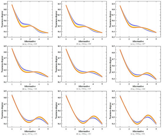
Figure 3.
Ranking results based on different values of parameters (CNEVs).
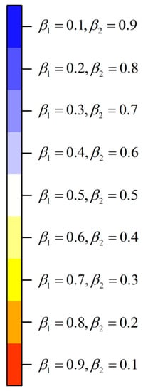
Figure 4.
The legend of Figure 3.
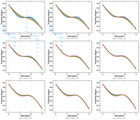
Figure 5.
Ranking results based on different values of parameters (MLNEVs).
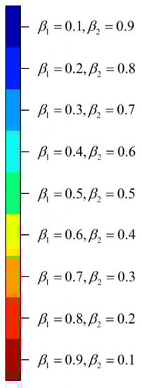
Figure 6.
The legend of Figure 5.
According to Figure 3 and Figure 4, the best alternative is always alternative 1. In the former four scenarios, the CNEV ranking results based on different values of parameters are consistent, sorted by . However, when and , the nearness degree of alternative 3 is greater than the nearness degree of alternative 2, and the ranking result is . Moreover, when and , the nearness degree of alternative 4 is greater than the nearness degree of alternative 3, and the ranking result is . In the latter five scenarios, when and , the ranking result starts to change to . Moreover, as the star rating and text review change, the difference between the nearness degrees of alternative 3 and alternative 4 grows larger. Therefore, parameters and have a greater effect on the ranking results, but parameters and have less influence on the sorting results.
According to Figure 5 and Figure 6, the MLNEV ranking results based on different values of parameters are consistent, sorted by , and alternative 6 is always the best in MLNEVs. However, as the star rating and text review change, the nearness degrees of alternative 7 and alternative 8 are close. When and , the nearness degree of alternative 8 starts to be greater than the nearness degree of alternative 7, and the ranking result is . The richness and dissimilarity slightly influenced the nearness degree in the former three scenarios in Figure 5 but did not affect the ranking results. Further, the richness and dissimilarity hardly affect the nearness degree in the latter six scenarios in Figure 5.
6. Conclusions
New energy vehicles have become popular, driven by the dual crises regarding the atmospheric environment and energy security. Since the automobile is a highly involved and high-value product, consumers tend to gather information through online reviews, which can assist in purchase decisions. This study takes the above new energy vehicle selection as a multi-attribute decision making problem. Firstly, we obtained text reviews and eight corresponding attribute star ratings for the five best-selling compact new energy vehicles (CNEVs) and the four best-selling mid–large new energy vehicles (MLNEVs) on the DCar website. Secondly, we designed adjustment rules to deal with the conflict of high star ratings but negative text reviews. Thirdly, we defined the concept of attribute richness and calculated attribute weights based on richness and dissimilarity. Finally, we classified consumers and recommended the optimal new energy vehicle for each consumer type. The results reveal that for CNEVs, consumers value comfort and the interior, while, for MLNEVs, they value power consumption and space. Then, for family-oriented consumers, car B and car H are recommended. For appearance-oriented and professional-oriented consumers, car A and car F are recommended. Finally, we conducted comparative and sensitivity analyses to ensure the effectiveness and robustness of the proposed approach.
There are some limitations. This study only obtained nine new energy vehicles from a single website and future research should consider the heterogeneity of websites and vehicles. Moreover, this study found a mismatch between the demands of review writers and review viewers. Consumer categorization and targeted recommendations were also conducted. However, future research should consider how to truly add the user attribute of the consumer type to websites, as well as conduct review filtering based on this.
Author Contributions
Conceptualization, S.Y. and X.Z.; methodology, S.Y., Z.D., Y.C. and X.Z.; software, X.Z.; validation, S.Y., Z.D. and Y.C.; formal analysis, X.Z.; investigation, Z.D. and X.Z.; data curation, S.Y., X.Z. and Z.D.; writing—original draft preparation, X.Z.; writing—review and editing, S.Y. and X.Z.; visualization, X.Z. and Z.D.; supervision, S.Y. and Y.C.; project administration, S.Y. and Y.C.; funding acquisition, S.Y. All authors have read and agreed to the published version of the manuscript.
Funding
This research was funded by the National Natural Science Foundation of China (No. 71901151 and No. 71991461).
Data Availability Statement
Prospective Economist, China Internet Network Information Center, Ai Media Consulting. The authors are willing to release specific data to readers if requested. Please contact the corresponding author for details.
Conflicts of Interest
The authors declare no conflict of interest.
Appendix A
Table A1.
The list of acronyms and their explanations.
Table A1.
The list of acronyms and their explanations.
| Acronym | Explanation |
|---|---|
| AHP | Analytic Hierarchical Process |
| CNEV | Compact New Energy Vehicle |
| COPRAS | Complex Proportional Assessment |
| DEST | Dempster–Shafer Evidence Theory |
| DI | Dissimilarity |
| ELECTRE | Elimination et Choix Traduisant la Realité, in French (Elimination and Choice Expressing Reality) |
| HFLTS | Hesitant Fuzzy Linguistic Term Set |
| LDA | Latent Dirichlet Allocation |
| LTS | Linguistic Term Set |
| MLNEV | Medium and Large New Energy Vehicle |
| MULTIMOORA | Multi-Objective Optimization by Ratio Analysis plus the full Multiplicative Form |
| OWA | Ordered Weighted Averaging |
| PLTS | Probabilistic Linguistic Term Set |
| PROMETHEE | Preference Ranking Organization Method for Enrichment of Evaluations |
| RI | Richness |
| SR | Star Ratings |
| TF-IDF | Term Frequency-Inverse Document Frequency |
| TODIM | Tomada de Decisao Interativa e Multicritévio, in Portuguese (Interactive and Multiple Criteria Decision Making) |
| TOPSIS | Technique for Order Preference by Similarity to Ideal Solution |
| TR | Text Reviews |
| VIKOR | Vise Kriterijumska Optimizacija Kompromisno Resenje, in Serbian (Multiple Criteria Optimization Compromise Solution) |
| WA | Weighted Averaging |
Table A2.
The star rating decision matrix (of CNEVs, attributes 1–4).
Table A2.
The star rating decision matrix (of CNEVs, attributes 1–4).
Table A3.
The star rating decision matrix (of CNEVs, attributes 5–8).
Table A3.
The star rating decision matrix (of CNEVs, attributes 5–8).
Table A4.
The star rating decision matrix (of MLNEVs, attributes 1–4).
Table A4.
The star rating decision matrix (of MLNEVs, attributes 1–4).
Table A5.
The star rating decision matrix (of MLNEVs, attributes 5–8).
Table A5.
The star rating decision matrix (of MLNEVs, attributes 5–8).
Table A6.
The text review decision matrix (of CNEVs, attributes 1–4).
Table A6.
The text review decision matrix (of CNEVs, attributes 1–4).
Table A7.
The text review decision matrix (of CNEVs, attributes 5–8).
Table A7.
The text review decision matrix (of CNEVs, attributes 5–8).
Table A8.
The text review decision matrix (of MLNEVs, attributes 1–4).
Table A8.
The text review decision matrix (of MLNEVs, attributes 1–4).
Table A9.
The text review decision matrix (of MLNEVs, attributes 5–8).
Table A9.
The text review decision matrix (of MLNEVs, attributes 5–8).
References
- Meng, W.D.; Ma, M.M.; Li, Y.Y.; Huang, B. New energy vehicle R&D strategy with supplier capital constraints under China’s dual credit policy. Energy Policy 2022, 168, 113099. [Google Scholar] [CrossRef]
- He, S.F.; Wang, Y.M. Evaluating new energy vehicles by picture fuzzy sets based on sentiment analysis from online reviews. Artif. Intell. Rev. 2023, 56, 2171–2192. [Google Scholar] [CrossRef]
- Cai, B.W. Deep Learning-Based Economic Forecasting for the New Energy Vehicle Industry. J. Math. 2021, 2021, 3870657. [Google Scholar] [CrossRef]
- Hua, Y.F.; Dong, F. How can new energy vehicles become qualified relays from the perspective of carbon neutralization? Literature review and research prospect based on the CiteSpace knowledge map. Environ. Sci. Pollut. Res. Int. 2022, 29, 55473–55491. [Google Scholar] [CrossRef]
- Wu, D.S.; Xie, Y.; Lyu, X.Y. The impacts of heterogeneous traffic regulation on air pollution: Evidence from China. Transp. Res. Part D Transp. Environ. 2022, 109, 103388. [Google Scholar] [CrossRef]
- Jiang, C.Q.; Duan, R.; Jain, H.K.; Liu, S.X.; Liang, K. Hybrid collaborative filtering for high-involvement products: A solution to opinion sparsity and dynamics. Decis. Support Syst. 2015, 79, 195–208. [Google Scholar] [CrossRef]
- Lin, B.Q.; Shi, L. Do environmental quality and policy changes affect the evolution of consumers’ intentions to buy new energy vehicles. Appl. Energy 2022, 310, 118582. [Google Scholar] [CrossRef]
- Abrahams, A.S.; Jiao, J.; Fan, W.G.; Wang, G.A.; Zhang, Z.J. What’s buzzing in the blizzard of buzz? Automotive component isolation in social media postings. Decis. Support Syst. 2013, 55, 871–882. [Google Scholar] [CrossRef]
- Xu, Z.G.; Dang, Y.Z.; Wang, Q.W. Potential buyer identification and purchase likelihood quantification by mining user-generated content on social media. Expert Syst. Appl. 2022, 187, 115899. [Google Scholar] [CrossRef]
- Liu, H.F.; Jayawardhena, C.; Osburg, V.-S.; Mohiuddin Babu, M. Do online reviews still matter post-purchase? Internet Res. 2020, 30, 109–139. [Google Scholar] [CrossRef]
- Yang, J.; Sarathy, R.; Lee, J. The effect of product review balance and volume on online Shoppers’ risk perception and purchase intention. Decis. Support Syst. 2016, 89, 66–76. [Google Scholar] [CrossRef]
- Soll, J.B.; Larrick, R.P. Strategies for Revising Judgment: How (and How Well) People Use Others’ Opinions. J. Exp. Psychol. Learn. Mem. Cogn. 2009, 35, 780–805. [Google Scholar] [CrossRef] [PubMed]
- Monaro, M.; Cannonito, E.; Gamberini, L.; Sartori, G. Spotting faked 5 stars ratings in E-Commerce using mouse dynamics. Comput. Hum. Behav. 2020, 109, 106348. [Google Scholar] [CrossRef]
- Zadeh, L.A. FUZZY SETS. Inf. Control 1965, 8, 338–353. [Google Scholar] [CrossRef]
- Zadeh, L.A. The concept of a linguistic variable and its application to approximate reasoning—I. Inf. Sci. 1975, 8, 199–249. [Google Scholar] [CrossRef]
- Zadeh, L.A. The concept of a linguistic variable and its application to approximate reasoning—II. Inf. Sci. 1975, 8, 301–357. [Google Scholar] [CrossRef]
- Zadeh, L.A. The concept of a linguistic variable and its application to approximate reasoning—III. Inf. Sci. 1975, 9, 43–80. [Google Scholar] [CrossRef]
- Rodríguez, R.; Martinez, L.; Herrera, F. Hesitant Fuzzy Linguistic Term Sets for Decision Making. IEEE Trans. Fuzzy Syst. 2012, 20, 109–119. [Google Scholar] [CrossRef]
- Zhu, B.; Xu, Z. Consistency Measures for Hesitant Fuzzy Linguistic Preference Relations. IEEE Trans. Fuzzy Syst. 2014, 22, 35–45. [Google Scholar] [CrossRef]
- Wei, C.P. A Multigranularity Linguistic Group Decision-Making Method Based on Hesitant 2-Tuple Sets. Int. J. Intell. Syst. 2016, 31, 612–634. [Google Scholar]
- Pang, Q.; Wang, H.; Xu, Z.S. Probabilistic linguistic term sets in multi-attribute group decision making. Inf. Sci. 2016, 369, 128–143. [Google Scholar] [CrossRef]
- Wang, Z.H.; Dong, X.Y. Determinants and policy implications of residents’ new energy vehicle purchases: The evidence from China. Nat. Hazards 2016, 82, 155–173. [Google Scholar] [CrossRef]
- Ma, S.C.; Fan, Y.; Feng, L.Y. An evaluation of government incentives for new energy vehicles in China focusing on vehicle purchasing restrictions. Energy Policy 2017, 110, 609–618. [Google Scholar] [CrossRef]
- Zhao, H.B.; Bai, R.B.; Liu, R.; Wang, H. Exploring purchase intentions of new energy vehicles: Do “mianzi” and green peer influence matter? Front. Psychol. 2022, 13, 951132. [Google Scholar] [CrossRef] [PubMed]
- Yetano Roche, M.; Mourato, S.; Fischedick, M.; Pietzner, K.; Viebahn, P. Public attitudes towards and demand for hydrogen and fuel cell vehicles: A review of the evidence and methodological implications. Energy Policy 2010, 38, 5301–5310. [Google Scholar] [CrossRef]
- Cai, M.S.; Tan, Y.J.; Ge, B.F.; Dou, Y.J.; Huang, G.; Du, Y.H. PURA: A Product-and-User Oriented Approach for Requirement Analysis from Online Reviews. IEEE Syst. J. 2022, 16, 566–577. [Google Scholar] [CrossRef]
- Liu, G.X.; Fan, S.Q.; Tu, Y.; Wang, G.J. Innovative Supplier Selection from Collaboration Perspective with a Hybrid MCDM Model: A Case Study Based on NEVs Manufacturer. Symmetry Basel 2021, 13, 143. [Google Scholar] [CrossRef]
- Nicolalde, J.F.; Cabrera, M.; Martinez-Gomez, J.; Salazar, R.B.; Reyes, E. Selection of a phase change material for energy storage by multi-criteria decision method regarding the thermal comfort in a vehicle. J. Energy Storage 2022, 51, 104437. [Google Scholar] [CrossRef]
- Yu, S.M.; Du, Z.J.; Wang, J.Q.; Luo, H.Y.; Lin, X.D. Trust and behavior analysis-based fusion method for heterogeneous multiple attribute group decision-making. Comput. Ind. Eng. 2021, 152, 106992. [Google Scholar] [CrossRef]
- Yu, S.M.; Du, Z.J.; Zhang, X.Y.; Luo, H.Y.; Lin, X.D. Trust Cop-Kmeans Clustering Analysis and Minimum-Cost Consensus Model Considering Voluntary Trust Loss in Social Network Large-Scale Decision-Making. IEEE Trans. Fuzzy Syst. 2022, 30, 2634–2648. [Google Scholar] [CrossRef]
- Yu, S.M.; Zhang, X.T.; Du, Z.J. Enhanced Minimum-Cost Consensus: Focusing on Overadjustment and Flexible Consensus Cost. Inf. Fusion 2023, 89, 336–354. [Google Scholar] [CrossRef]
- Zheng, J.; Wang, Y.M.; Zhang, K. Solution of heterogeneous multi-attribute case-based decision making problems by using method based on TODIM. Soft Comput. 2020, 24, 7081–7091. [Google Scholar] [CrossRef]
- Yu, S.M.; Du, Z.J.; Xu, X.H. Hierarchical Punishment-Driven Consensus Model for Probabilistic Linguistic Large-Group Decision Making with Application to Global Supplier Selection. Group Decis. Negot. 2021, 30, 1343–1372. [Google Scholar] [CrossRef]
- Huang, J.Y.; Jiang, N.Y.; Chen, J.; Balezentis, T.; Streimikiene, D. Multi-criteria group decision-making method for green supplier selection based on distributed interval variables. Econ. Res. Ekon. Istraživanja 2022, 35, 746–761. [Google Scholar] [CrossRef]
- Yu, S.M.; Wang, J.; Wang, J.Q.; Li, L. A multi-criteria decision-making model for hotel selection with linguistic distribution assessments. Appl. Soft Comput. 2018, 67, 741–755. [Google Scholar] [CrossRef]
- Giri, B.C.; Molla, M.U.; Biswas, P. TOPSIS Method for Neutrosophic Hesitant Fuzzy Multi-Attribute Decision Making. Informatica 2020, 31, 35–63. [Google Scholar] [CrossRef]
- Nobre, F.F.; Trotta, L.T.F.; Gomes, L. Multi-criteria decision making—An approach to setting priorities in health care. Stat. Med. 1999, 18, 3345–3354. [Google Scholar] [CrossRef]
- Opricovic, S.; Tzeng, G.H. Multicriteria planning of post-earthquake sustainable reconstruction. Comput. Aided Civ. Infrastruct. Eng. 2002, 17, 211–220. [Google Scholar] [CrossRef]
- Roy, B. The outranking approach and the foundations of electre methods. Theory Decis. 1991, 31, 49–73. [Google Scholar] [CrossRef]
- Brauers, W.K.M.; Zavadskas, E.K. Project management by multimoora as an instrument for transition economies. Technol. Econ. Dev. Econ. 2010, 16, 5–24. [Google Scholar] [CrossRef]
- Agrebi, M.; Abed, M. Decision-making from multiple uncertain experts: Case of distribution center location selection. Soft Comput. 2021, 25, 4525–4544. [Google Scholar] [CrossRef]
- Zhang, K.; Zheng, J.; Wang, Y.M. A heterogeneous multi-attribute case retrieval method based on neutrosophic sets and TODIM for emergency situations. Appl. Intell. 2022, 52, 15177–15192. [Google Scholar] [CrossRef] [PubMed]
- Wen, Z.; Xiong, Z.M.; Lu, H.; Xia, Y.P. Optimisation of Treatment Scheme for Water Inrush Disaster in Tunnels Based on Fuzzy Multi-criteria Decision-Making in an Uncertain Environment. Arab. J. Sci. Eng. 2019, 44, 8249–8263. [Google Scholar] [CrossRef]
- Wang, S.L.; Qu, S.J.; Goh, M.; Wahab, M.I.M.; Zhou, H. Integrated Multi-stage Decision-Making for Winner Determination Problem in Online Multi-attribute Reverse Auctions under Uncertainty. Int. J. Fuzzy Syst. 2019, 21, 2354–2372. [Google Scholar] [CrossRef]
- Abu Dabous, S.; Zeiada, W.; Zayed, T.; Al-Ruzouq, R. Sustainability-informed multi-criteria decision support framework for ranking and prioritization of pavement sections. J. Clean. Prod. 2020, 244, 118755. [Google Scholar] [CrossRef]
- Yang, Y.P.; Liu, Z.Q.; Chen, H.M.; Wang, Y.Q.; Yuan, G.H. Evaluating Regional Eco-Green Cooperative Development Based on a Heterogeneous Multi-Criteria Decision-Making Model: Example of the Yangtze River Delta Region. Sustainability 2020, 12, 3029. [Google Scholar] [CrossRef]
- Wang, J.Q.; Zhang, X.H. A Novel Multi-Criteria Decision-Making Method Based on Rough Sets and Fuzzy Measures. Axioms 2022, 11, 275. [Google Scholar] [CrossRef]
- Fan, Z.P.; Li, G.M.; Liu, Y. Processes and methods of information fusion for ranking products based on online reviews: An overview. Inf. Fusion 2020, 60, 87–97. [Google Scholar] [CrossRef]
- Fan, Z.P.; Xi, Y.; Liu, Y. Supporting consumer’s purchase decision: A method for ranking products based on online multi-attribute product ratings. Soft Comput. 2018, 22, 5247–5261. [Google Scholar] [CrossRef]
- Liu, P.D.; Teng, F. Probabilistic linguistic TODIM method for selecting products through online product reviews. Inf. Sci. 2019, 485, 441–455. [Google Scholar] [CrossRef]
- Bi, J.W.; Liu, Y.; Fan, Z.P. Representing sentiment analysis results of online reviews using interval type-2 fuzzy numbers and its application to product ranking. Inf. Sci. 2019, 504, 293–307. [Google Scholar] [CrossRef]
- Sharma, H.; Tandon, A.; Kapur, P.K.; Aggarwal, A.G. Ranking hotels using aspect ratings based sentiment classification and interval-valued neutrosophic TOPSIS. Int. J. Syst. Assur. Eng. Manag. 2019, 10, 973–983. [Google Scholar] [CrossRef]
- Zhang, C.X.; Zhao, M.; Cai, M.Y.; Xiao, Q.R. Multi-stage multi-attribute decision making method based on online reviews for hotel selection considering the aspirations with different development speeds. Comput. Ind. Eng. 2020, 143, 106421. [Google Scholar] [CrossRef]
- Zhang, D.; Li, Y.L.; Wu, C. An extended TODIM method to rank products with online reviews under intuitionistic fuzzy environment. J. Oper. Res. Soc. 2020, 71, 322–334. [Google Scholar] [CrossRef]
- Zhang, C.; Tian, Y.X.; Fan, L.W.; Li, Y.H. Customized ranking for products through online reviews: A method incorporating prospect theory with an improved VIKOR. Appl. Intell. 2020, 50, 1725–1744. [Google Scholar] [CrossRef]
- Song, Y.M.; Li, G.X.; Li, T.; Li, Y.H. A purchase decision support model considering consumer personalization about aspirations and risk attitudes. J. Retail. Consum. Serv. 2021, 63, 102728. [Google Scholar] [CrossRef]
- Dahooie, J.H.; Raafat, R.; Qorbani, A.R.; Daim, T. An intuitionistic fuzzy data-driven product ranking model using sentiment analysis and multi-criteria decision-making. Technol. Forecast. Soc. Chang. 2021, 173, 121158. [Google Scholar] [CrossRef]
- Yang, Z.L.; Gao, Y.; Fu, X.L. A decision-making algorithm combining the aspect-based sentiment analysis and intuitionistic fuzzy-VIKOR for online hotel reservation. Ann. Oper. Res. 2021. [Google Scholar] [CrossRef] [PubMed]
- Qin, J.D.; Zeng, M.Z. An integrated method for product ranking through online reviews based on evidential reasoning theory and stochastic dominance. Inf. Sci. 2022, 612, 37–61. [Google Scholar] [CrossRef]
- Bi, J.W.; Han, T.Y.; Yao, Y.B.; Li, H. Ranking hotels through multi-dimensional hotel information: A method considering travelers’ preferences and expectations. Inf. Technol. Tour. 2022, 24, 127–155. [Google Scholar] [CrossRef]
- Tayal, D.K.; Yadav, S.K.; Arora, D. Personalized ranking of products using aspect-based sentiment analysis and Plithogenic sets. Multimed. Tools Appl. 2022, 82, 1261–1287. [Google Scholar] [CrossRef]
- Tversky, A.; Kahneman, D. Judgment under uncertainty—Heuristics and biases. Science 1974, 185, 1124–1131. [Google Scholar] [CrossRef]
- Stanovich, K.E.; West, R.F. Individual differences in reasoning: Implications for the rationality debate? Behav. Brain Sci. 2000, 23, 645–726. [Google Scholar] [CrossRef] [PubMed]
- Cho, H.S.; Sosa, M.E.; Hasija, S. Reading Between the Stars: Understanding the Effects of Online Customer Reviews on Product Demand. MSom Manuf. Serv. Oper. Manag. 2021, 24, 1887–2386. [Google Scholar]
- Gavilan, D.; Avello, M.; Martinez-Navarro, G. The influence of online ratings and reviews on hotel booking consideration. Tour. Manag. 2018, 66, 53–61. [Google Scholar] [CrossRef]
- Hong, S.; Pittman, M. eWOM anatomy of online product reviews: Interaction effects of review number, valence, and star ratings on perceived credibility. Int. J. Advert. 2020, 39, 892–920. [Google Scholar] [CrossRef]
- Hwang, C.-L.; Yoon, K. Multiple Attribute Decision Making: Methods and Applications—A State-of-the-Art Survey. In Lecture Notes in Economics and Mathematical Systems; Springer: Berlin/Heidelberg, Germany, 1981. [Google Scholar]
- Chen, X.H.; Zhang, W.W.; Xu, X.H.; Cao, W.Z. Managing Group Confidence and Consensus in Intuitionistic Fuzzy Large Group Decision-Making Based on Social Media Data Mining. Group Decis. Negot. 2022, 31, 995–1023. [Google Scholar] [CrossRef]
- Hu, J.H.; Zhang, X.H.; Yang, Y.; Liu, Y.M.; Chen, X.H. New doctors ranking system based on VIKOR method. Int. Trans. Oper. Res. 2020, 27, 1236–1261. [Google Scholar] [CrossRef]
- Li, Y.; Zhang, Y.X.; Xu, Z.S. A Decision-Making Model Under Probabilistic Linguistic Circumstances with Unknown Criteria Weights for Online Customer Reviews. Int. J. Fuzzy Syst. 2020, 22, 777–789. [Google Scholar] [CrossRef]
- Yen, J. Generalizing the dempster shafer theory to fuzzy-sets. IEEE Trans. Syst. Man Cybern. 1990, 20, 559–570. [Google Scholar] [CrossRef]
Disclaimer/Publisher’s Note: The statements, opinions and data contained in all publications are solely those of the individual author(s) and contributor(s) and not of MDPI and/or the editor(s). MDPI and/or the editor(s) disclaim responsibility for any injury to people or property resulting from any ideas, methods, instructions or products referred to in the content. |
© 2023 by the authors. Licensee MDPI, Basel, Switzerland. This article is an open access article distributed under the terms and conditions of the Creative Commons Attribution (CC BY) license (https://creativecommons.org/licenses/by/4.0/).