Article

Constructing an Evolutionary Tree and Path–Cycle Graph Evolution along It

by
Konstantin Gorbunov
* and
Vassily Lyubetsky
Institute for Information Transmission Problems of the Russian Academy of Sciences, 127051 Moscow, Russia
*
Author to whom correspondence should be addressed.
Partial support of RFBR grant 20-01-00670 acknowledged.
Mathematics 2023, 11(9), 2024; https://doi.org/10.3390/math11092024
Submission received: 29 March 2023 / Revised: 19 April 2023 / Accepted: 21 April 2023 / Published: 24 April 2023
(This article belongs to the Special Issue Mathematical Logic, Algorithms and Applications)

Abstract

:
The paper solves the problem of constructing an evolutionary tree and the evolution of structures along it. This problem has long been posed and extensively researched; it is formulated and discussed below. As a result, we construct an exact cubic-time algorithm which outputs a tree with the minimum cost of embedding into it and of embedding it into a given network (Theorem 1). We construct an algorithm that outputs a minimum embedding of a tree into a network, taking into account incomplete linear sorting; the algorithm depends linearly on the number of nodes in the network and is exact if the sorting cost is not less than the sum of the duplication cost and the loss cost (Theorem 3). We construct an exact approximately quadratic-time algorithm which, for arbitrary costs of SCJ operations, solves the problem of reconstruction of given structures on any two-star tree (Theorem 4). We construct an exact algorithm which reduced the problem of DCJ reconstruction of given structures on any star to a logarithmic-length sequence of SAT problems, each of them being of approximately quadratic size (Theorem 5). The theorems have rigorous and complete proofs of correctness and complexity of the algorithms, and are accompanied by numerical examples and numerous explanatory illustrations, including flowcharts.

1. General Introduction

Tree graphs arise very widely, both in fundamental problems of discrete mathematics and in applied problems from very different subject areas; for particular examples of their use, see [1,2]. Such a problem is the classification problem and well-known methods for constructing graph trees, such as the ID3 algorithm; see, e.g., [3,4]. Note the applications of random trees and random forests in [5].
In the present paper, we consider a specific problem of constructing the evolution of structures along a tree or network G; G is understood as the discrete time in which the evolution progresses. This problem naturally decomposes into two parts, the construction of this G (Theorems 1–3) and the construction along it of the evolution of X, itself from the given X0 at the leaves of the tree (Theorems 4 and 5). The construction of G also requires some kind of a priori data; in particular, G is constructed as a tree/network that is optimally coordinated with already known trees or networks P and S so that there are optimal embeddings PGS. This problem setting is well known, and hundreds of papers, surveys, and books are devoted to various versions of it, of which we note the survey ([6] Section 5) and the book [7]. The present paper is not a survey and contains proofs of the four theorems mentioned above. Algorithms for constructing the discrete evolution of structures along a tree are often heuristic. In our purely mathematical study, all algorithms have complete and rigorous proofs of their correctness and of low estimates of their computational complexity.
Evolution analysis is one of the most fundamental mathematical problems, having, at the same time, a broad practical importance. In this respect, we have considered discrete evolution, where a rooted tree acts as time. This understanding of time is particularly important in connection with biological evolution, although, in this paper, evolution is considered purely mathematically, without any relation to various applications. We consider two phases of reconstruction to necessarily following each other, first, a tree acting as time is constructed, and then evolution itself is sought for along the constructed tree. Namely, the first problem consists of constructing a tree as the “average” between a given tree and a given network, which reduces to minimizing a given functional defined on all trees of a fixed size. In other words, the first problem involves creating a new tree that represents an “average” between a tree and a network (in particular, also a tree). This is completed by finding a tree that minimizes a given functional, which assigns a value to each possible tree of a fixed size. The goal is to find the tree minimizing this value that will be the best representation of the “average” between these two given graphs. The second problem consists of describing the evolution of structures defined at leaves of a given tree. Evolution is understood as the continuation of these structures onto internal nodes of the tree, where the continuation is the minimum of a given functional defined on all arrangements along the tree. An arrangement is a one-to-one mapping of structures to internal nodes of the tree, together with already fixed structures at its leaves. In other words, the second problem aims to explain how structures that are defined at the leaves of a tree evolve over time by continuing onto internal nodes of the tree. The continuation of these structures is determined by finding the arrangement that minimizes a given functional, which is defined for all possible arrangements along the tree. Essentially, the goal is to find the best possible way for the structures to evolve along the tree. In addition to the functional, the notion of a structure must be defined. In this paper, a structure is a loaded directed graph consisting of paths and cycles (a path–cycle graph). Of course, both problems can be considered in the framework of other formulations as well.
In Section 2, “Tree Construction,” we prove Theorem 1, where we construct an exact cubic-time algorithm which, given a binary tree P, binary tree or network S, and a collection B of sets, outputs a binary tree G minimizing the sum of costs of minimum continuations that preserve the natural ordering of leaf mappings from P to G and from G to S, provided that G contains only clades that belong to B. Here, a clade means the set of all leaves below any given node gG. A continuation preserving the natural ordering, PG or GS, is called an embedding; thus, here we minimize the sum of costs of two minimum embeddings. Our mathematical results (Theorems 1–5), which develop the problem of discrete optimization, are used by us, in particular, in applied biological works to construct the evolution of genomes and genomic rearrangement. For example, the algorithm from Theorem 1 allows us to trace the evolution of proteins with respect to the genes that encode them, and, at the same time, the evolution of these genes with respect to the species that contain them. The example described in Section 2.6 (and in our applied works) show that this algorithm significantly improves the intermediate tree G compared to what the algorithm in [8] produces for precisely the same data. That algorithm is based on building the optimal gene tree by applying modifications on the input tree P guided by the tree S. Thus, the algorithm in [8] is based on descending to the local minimum of a functional starting from a tree G equal to the given tree P. The algorithm in [8] is quite different from ours and, moreover, is heuristic; the latter also makes it drastically different from our algorithm. In [8], no proofs or considerations about the exactness of that algorithm are given, but only a quadratic estimate of its runtime.
In Section 2, we also construct a minimum embedding of a tree into a network taking into account duplication, loss, and Incomplete Linear Sorting events (Theorem 3). Transition to a network S instead of a tree S significantly extends the average tree problem in mathematical and applied aspects. Previously, for this problem an algorithm in [9] was known, which took into account only one Incomplete Linear Sorting event.
In Section 3, “Reconstruction of Structures on a Tree,” we prove two theorems. In Theorem 4, we construct an exact approximately quadratic-time algorithm which solves the SCJ reconstruction problem on any two-star tree for arbitrary costs of SCJ operations. In Theorem 5, we construct an exact algorithm which, on any star, for arbitrary costs of DCJ operations, reduces a cyclic equal-content DCJ reconstruction problem to a logarithmic-length sequence of SAT (Boolean satisfiability) problems, each of them being approximately quadratic-size. For example, algorithms from Theorems 4 and 5 make it possible to reconstruct genomes of ancestral organisms and genomic rearrangements. Previously, an exact SCJ reconstruction algorithm was developed only for equal cost operations in [10] or on a star-like tree in [11], and the DCJ reconstruction algorithm was developed as a reduction in the reconstruction problem to an integer linear programming problem in [12].
The rest of this article is organized as follows. Section 2 contains definitions related to the embedding of a tree into a network (Section 2.1); setting of the intermediate tree problem and the formulation of Theorem 1 (Section 2.2); the definition of embedding a tree into a network (Section 2.3); a description of the algorithm for constructing an intermediate tree and a Proof of Theorem 1 (Section 2.4); a description of the choice of the main parameter of the algorithm (Section 2.5); an example of the algorithm (Section 2.6); a description of the algorithm for constructing an embedding of a tree into a network, taking into account “Incomplete Linear Sorting”, along with a Proof of Theorem 3 (Section 2.7); and, finally, an example of the operation of the algorithm (Section 2.8).
Section 3 contains a setting of the structure reconstruction problem and formulations of Theorems 4 and 5 (Section 3.1), a description of the SCJ reconstruction algorithm on a two-star tree (Section 3.2), a proof of the exactness of this algorithm and estimates of its runtime (Theorem 4, Section 3.3), an example of the operation of the SCJ reconstruction algorithm (Section 3.4), a description of the SCJ reconstruction algorithm for the cyclic case of the problem (Section 3.5), a description of the DCJ reconstruction algorithm on a star and a Proof of Theorem 5 (Section 3.6), an example of the DCJ reconstruction algorithm (Section 3.7), and a description of the choice of parameters for this algorithm (Section 3.8).
Section 4 (Discussion) briefly mentions one of the possible applications of our algorithms, as well as possible directions for further mathematical research related to this work. In general, the issue of applications of these algorithms requires descriptions of the corresponding subject areas and is far in style and content from the presented mathematical study.

2. Tree Construction

2.1. Introduction

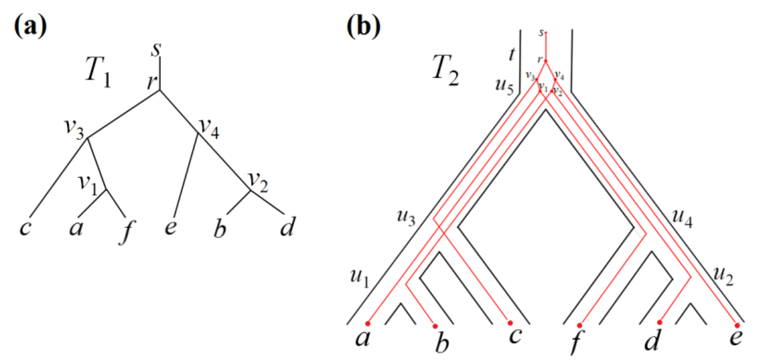
We consider rooted trees; a root is entered by an edge which starts at a node of degree 1, referred to as a super-root; the edge itself will be called the root edge. We will regard the super-root of a tree, and then the root, as located “at the top,” and leaves of a tree (all of degree 1) as located “at the bottom”, as shown in Figure 1a. Similarly, subtrees are regarded with their root edge, which enters the root of the subtree and starts at its super-root, the latter being of degree 1. The tail of an edge e is its endpoint located closer to the root, and the second endpoint is the head of the edge; they are denoted by e+ and e, respectively. An ancestor node/edge is located closer to the root, and a descendant node/edge is farther from the root, both lying on the same path; this relation is denoted by ≤. The nearest ancestor is called a parent, and the nearest descendant is called a child; nodes located immediately below the same node are said to be sibling nodes, each of them is called a sister of any other one. In essence, a tree specifies a parent–child relation. For any set N of leaves, a node which is the lowest among all ancestors of all leaves in N is well defined. Denote it by N′. For two trees T1 and T2, there is a well-known canonical continuation [13,14] of any preassigned mapping s from leaves in T1 to leaves in T2, which is denoted here by s″. Namely, for an interior node x in T1 with a set x< of leaves lying below it, we let s″(x) = s(x<)′. The set x< is called the clade of x, or the clade of the root edge entering x, or the clade of the subtree defined by x.
If s″(e+) = s″(e), then s′(e+) is defined as the edge entering s″(e) from above; for instance, s′ maps the super-root in T1 into the root edge in T2. Thus, s′ maps nodes in T1 into nodes and edges in T2; see Figure 1b. This definition can be generalized to the case where T2 is a network (see Section 2.3). We will refer to the mapping s′ as an embedding of T1 into T2. Below, when saying “a tree T1 is mapped to a tree T2,” we always mean precisely this mapping s′ and speak about its images and arguments. Note that in this case we have a preassigned mapping s, which is called a leaf mapping. Of course, the mapping s′ preserves the natural order.
The path of an edge eT1 in a tree T2 is a path consisting of nodes in T2 from s′(e+) to s′(e) excluding its endpoints s′(e+) and s′(e).
The image tree of T1 in T2 is defined to be a tree isomorphic to T1 with nodes located at nodes and in edges of T2 so that v is located either at the node s′(v) or in the pipe t = s′(v) (see Figure 2). In this sense, edges of T2 will be referred to as pipes containing nodes and edges of T1. Images are connected by an edge according to the parent–child relation of their arguments. Thus, we want to consider an image tree as the T1 tree located inside T2. Our use of mathematical interpretations in embedding is related to our inspiration from biological paradigms, such as the evolution of genomes and genomic rearrangement.
If tree leaves are assigned unique names, we may not distinguish between a leaf and a name assigned to it. A tree with labelled leaves represents the discrete-time evolution of a matter which is assigned to the root of the tree; the evolution goes from the root to leaves through interior nodes of the tree. For example, this can be evolution of a gene, protein, species, etc., from the root along the whole given tree to its leaves, which represent up-to-date states of the initial (at the root) matter; such up-to-date states could already be actually specified.
Evolution analysis is one of the most fundamental mathematical problems, having at the same time a broad practical importance (see, e.g., [15,16,17,18]). Note, also, the work [19], which describes an algorithm for solving the problem of isomorphic tree embedding in a network and provides numerous references to articles related to this topic. A detailed overview of topics related to evolutionary trees and numerous references are given in [6]. Issues related to phylogenetic networks are discussed in the book [7].
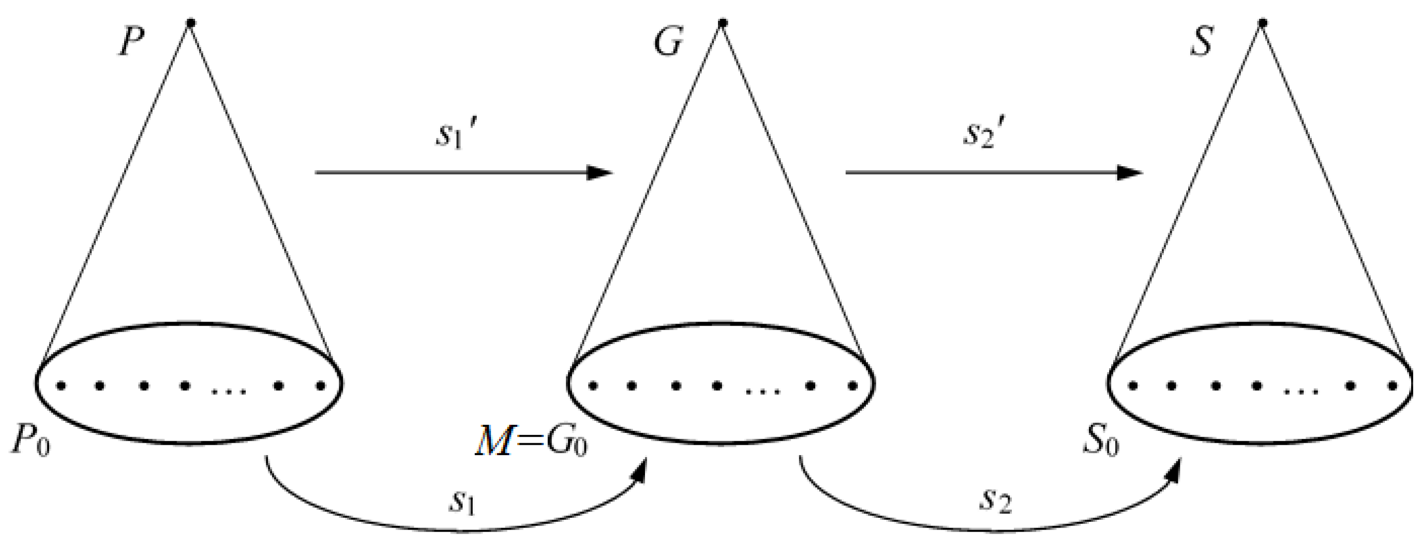
Let T0 be the set of all leaves of a tree or network T. The problem is as follows: given a tree P, a set M, a tree or network S, and mappings s1: P0M and s2: MS0, find a tree G (where G0 = M) that reconciles the evolutions s1′ and s2′ in the following sense. We define costs c(s′) and c(s2′) of the embeddings s1′: PG and s2′: GS, respectively, and then minimize f(G) = c(s1′) + c(s2′) with respect to the argument G (see Figure 3). For the case of a network S, the definition of the embedding cost of s2′: GS is given in Section 2.7. Until that section, S will always be a tree, and the embedding costs will be considered according to Definitions 1 and 2 below. However, f(G) can be defined to be an easily computable function with some properties that we will need below.
We are dealing here with a general mathematical problem, so all further material is presented independently of any applications. However, as a typical example, let us describe its content using biological terms. Let P be a tree whose leaves are assigned with protein names (“protein evolution tree”, or, for short, protein tree), and let S be a network, in particular a tree, whose leaves are assigned with names of species containing these proteins (“species evolution network”, or, for short, species network/tree). For more details concerning the notion of a network, see Section 2.3. At this moment, we may assume S to be a tree. Let M be a set of genes from which proteins in leaves of P are formed, and let a leaf mapping s1: P0M be fixed where y = s1(x) is the gene from which a protein x is formed (see Figure 3). On the other hand, a mapping s2: MS0 is fixed where s2(y) is the species to which a gene y belongs. The composition s2(s1): P0S0 defines a mapping which specifies a species to which a protein x belongs. s1 and s2 are specified extrinsically for applied reasons. Let G be a tree with leaf set M = G0, which is called the “gene evolution tree”, or gene tree, or an intermediate tree with respect to P and S. Given s1 and s2, their continuations s1′: PG and s2′: GS are defined. We regard s1′ as evolution of proteins relative to genes (in the gene tree), and s2′ as evolution of genes relative to species (in the species tree). The problem is to minimize c(s1′) + c(s2′) with respect to the gene tree G and, as a result, to find a tree G* on which c(s1′) + c(s2′) attains its minimum value.

2.2. Setting of the Intermediate Tree Problem and Formulation of Theorem 1

Let the degree of every node in the trees T1 and T2 except for the super-root and leaves be 3. All leaves are labeled with unique names, and M is the set of leaves together with their names in T2.
The embedding s′: T1T2 for the trees T1 and T2 is defined above.
Definition 1.
A duplication in T1 is a node of degree 3 which is mapped to a pipe. Informally, for example, the node r ∈ T1 in Figure 4a has an image located in a pipe above the images of the children v7 ∈ T1 and v6 ∈ T1, which is interpreted as a furcation of the node r in this pipe into v7 and v6. A loss is a pair consisting of an edge e ∈ T1 and a node y ∈ T2 such that y belongs to the path of e in T2 (the path does not contain the images s′(e+) and s′(e), the extreme nodes of the path). Informally, an edge e passes through y and has no furcation in y. A loss is said to be implicit if a clade of one of the child pipes of y does not contain images of leaves from T1, otherwise it is said to be explicit. We define the locus of a duplication to be its image and the locus of a loss to be the node y. Duplications and losses will be called evolutionary events. For example, all events for the T1 tree shown in Figure 1 are presented in Figure 4. Let each event be assigned with its cost, a strictly positive rational number. The cost c(s′) of an embedding s′ is the total cost of all its events. These definitions can be carried over to the case where S is a network (see Section 2.3).
The intermediate tree problem is as follows: given a tree P and a tree/network S together with leaf mappings s1: P0M and s2: MS, find a tree G with leaf set M = G0 for which the sum of the costs of the embeddings s1′: PG and s2′: GS is minimal. Under Definition 1, the problem consists of minimizing the total number of events that occur in these two evolutions taking into account their costs. This number c(s1′) + c(s2′) is called the cost of a tree G. The problem setting is not yet completed if S is a network; in this case we also need to define the continuation s2′: GS of the mapping s2. We define it in Section 2.3 below, where it is called the minimum embedding; in the case of a tree, there is exactly one minimum embedding, i.e., the embedding s′ defined in Section 2.1. The main feature of a minimum embedding in the case of a network is the fact that it is not defined uniquely; there exist many minimum embeddings.
The problem for the case of a tree S was posed in [8], where it was proved that the problem is NP-hard. The latter means that it cannot be solved by any polynomial algorithm if P ≠ NP. However, a polynomial algorithm or even a low-complexity algorithm can be found if we introduce some additional conditions into the problem. In [8], the problem for a tree was solved by a heuristic (quadratic-complexity) algorithm given that the mapping s1 is injective; moreover, that algorithm did not assume the costs of events. Instead, we suggest another condition.
(*) The tree G contains only clades from a fixed-in-advance collection B of non-empty subsets of M such that B contains M itself and all its one-element subsets, and any non-one-element set A in B has a partition in B.
The latter means that A can be partitioned into two non-empty disjoint parts from B; in particular, B does not contain the empty set. In Section 2.5, we explain how one can construct a collection B satisfying condition (*).
Under this condition, we obtain an exact (cubic-complexity) algorithm solving this problem for both a tree and a network S. Even for the case of a tree, our algorithm is other than that in [8]. Additionally, for the case of a network we propose an algorithm finding one particular minimum embedding which is denoted by s2′: GS.
Thus, below, we prove the following.
Theorem 1.
An exact cubic-time (in the input data size) algorithm is construct which, given a binary tree P, binary tree S, and a collection B of subsets of M, outputs a binary tree G minimizing the sum of costs of embeddings of P to G and of G to S provided that G contains only clades from B.
Theorem 2.
An exact cubic-time (in the input data size) algorithm is constructed which, given a binary tree P, binary network S, and a collection B of subsets of M, outputs a binary tree G and a minimum embedding s2′ minimizing the sum of costs of embeddings of P to G and of G to S provided that G contains only clades from B.
To conclude this subsection, we note that the practical relevance of this problem is, in particular, explained in [8], where extensive references to the history of the intermediate tree problem in the context of bioinformatics are provided. The definition of a mapping from one tree to another, known in the literature as “alpha mapping,” was proposed in the mid-1990s in [13,14]. For the case of trees T1 and T2, linear time algorithms for constructing a unique embedding s′: T1T2 are known [20,21].

2.3. Definition of an Embedding of a Tree into a Network

Definition 2.
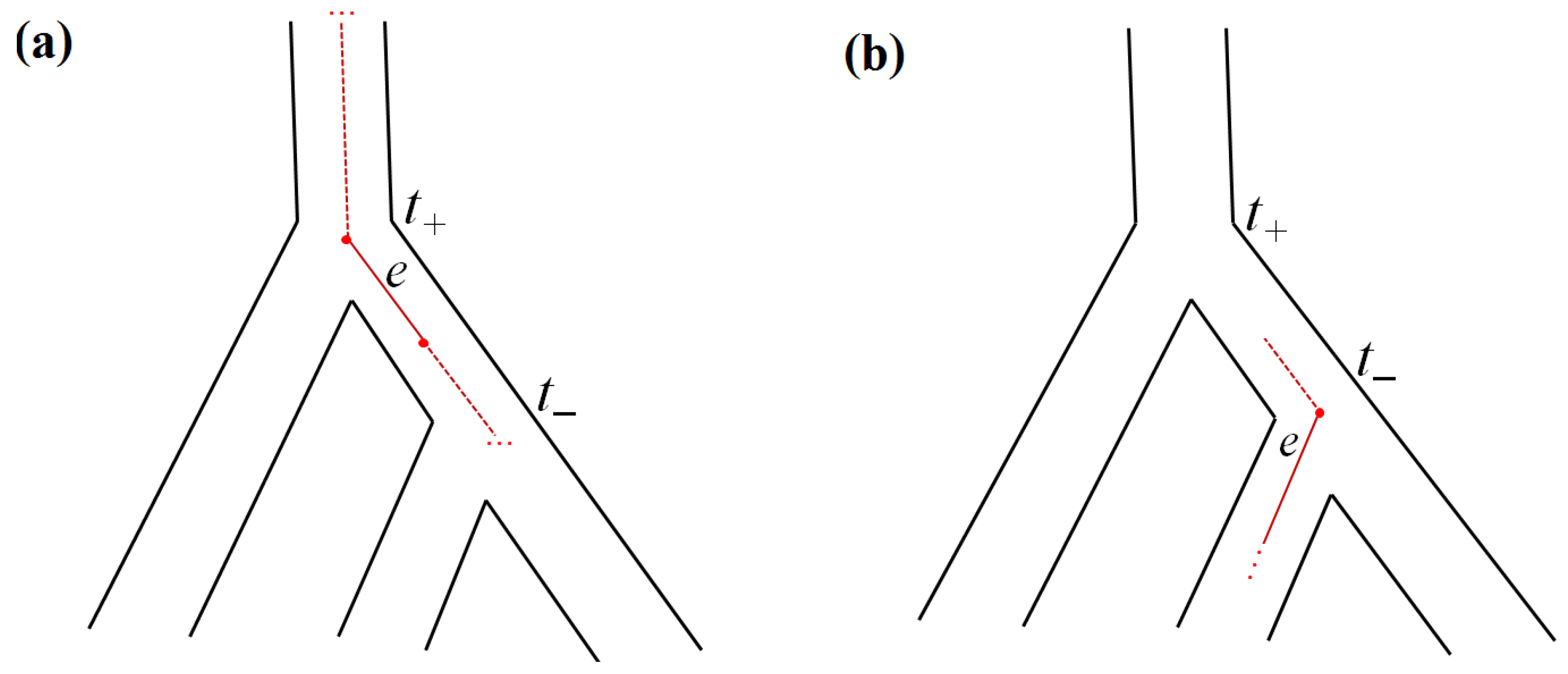
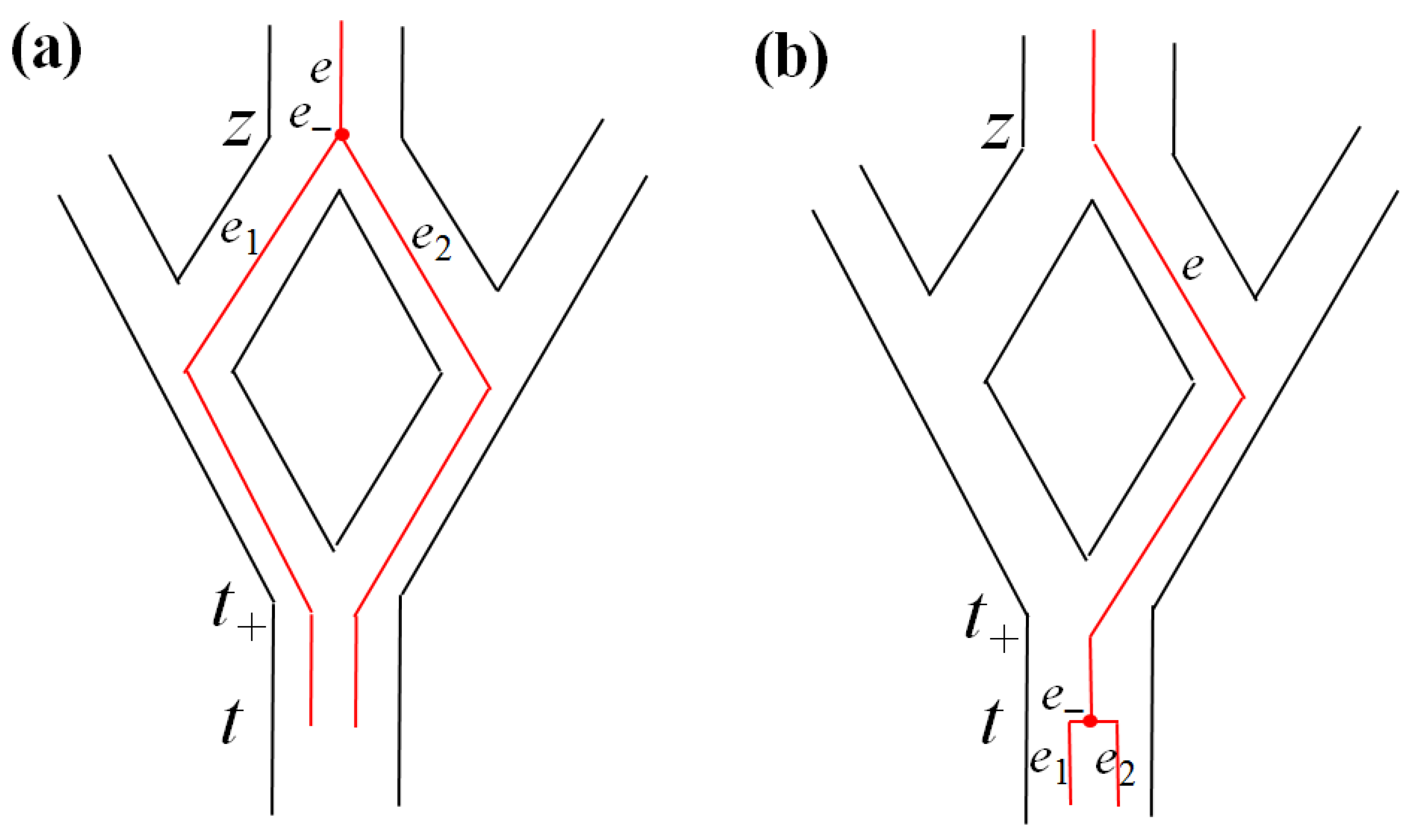
Let s′: T1 → T2 be an embedding. Recall that edges in T2 are referred to as pipes. An edge e ∈ T1 enters a pipe t ∈ T2 if s′ maps e+ to t+ or above t+ and maps e to t or below t. Informally, in the image tree, the edge e persists at t+ and either becomes lost inside t or goes further through the whole t (see Figure 5a). Similarly, an edge e leaves a pipe t ∈ T2 if s′ maps e+ to t or above and maps e strictly below t. Informally, in the image tree, the edge e arises at t or above and persists in one of the child pipes of t, maybe partially (see Figure 5b). Such a description is called an evolutionary scenario of T1 in T2.
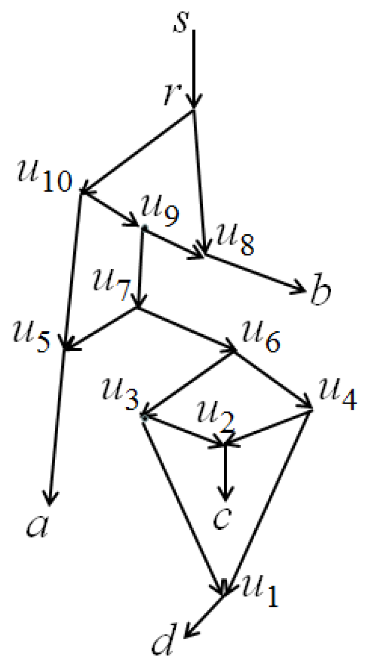
From binary network S, we understand a directed acyclic graph with nodes divided into four groups, one node of in-degree 0 and out-degree 1 (the super-root), nodes of in-degree 1 and out-degree 2 (tree-type nodes, including the root), nodes of in-degree 2 and out-degree 1 (hybrid nodes), and nodes of in-degree 1 and out-degree 0 (leaves). Thus, a tree is a particular case of a network with no hybrid nodes. A node may have two parents, so the notion of a nearest common ancestor is not well defined (see Figure 6). If there is a directed path from node x to node y, then we say that x is above y and write xy or yx. A hybrid pipe t is a pipe whose endpoint t is a hybrid node. A tree-type pipe is defined similarly.
The continuation of this order onto all nodes and pipes, which is also written as x is above y (xy) or y is below x (yx), is defined similarly. For example, pipe e is below e+ and above e. Sometimes, the term ancestor is used instead of above, and descendant is used instead of below; a node located immediately above some node is called its parent, and a node located immediately below some node is called its child; nodes located immediately below the same node are said to be sibling nodes; each of them is called a sister of any other one.
A subnetwork Sx is the network consisting of a node x and everything that lies below it, together with a root pipe (for Sx) entering x from above; if there are two such pipes, choose any of them. The leaf set in Sx is called a clade in S or the clade of the node x, or also the clade of the root pipe entering x; we denote the clade of x by x<. A subnetwork may contain nodes with two parents, such that one of them does not belong to Sx. Such nodes of a subnetwork will still be referred to as hybrid nodes. Throughout what follows, by a network we mean a rooted binary network with a root pipe, and similarly for a subnetwork.
As in the case of two trees, for a tree G and a network S we define a continuation s″ of a mapping s from leaves in G to leaves in S, though, on interior nodes, the value of s″ can also be a pipe in S. Namely, let a continuation s″ from nodes in G to nodes and pipes in S be any continuation of s preserving the natural ordering ≤ in G and having the following properties, the super-root in G is mapped to the root pipe in S; and the image y = s″(x) of a node x is not a hybrid node. If s″(x) is a tree-type node, then the paths px-x1 and px-x2 of the child edges of x enter different child pipes of s″(x). Moreover, the mapping s″ for any edge eG is complemented with pointing to a directed path pe which consists of nodes in S leading from s″(e+) to s″(e). An example in Figure 7b is the node e, which is mapped to t. For the case of a tree, such a path pe is unique; above, it was called the path of the edge e. Such a non-unique s″ will be called an embedding of a tree G into a network S.
Now we will repeat Definitions 1 and 2 for a network. An edge eG enters a pipe tS if s″ maps e+ to t+ or above t+, maps e to t or below t, and pe passes through t, maybe partially. Similarly, an edge e leaves a pipe t if s″ maps e+ to t or above t, maps e strictly below t, and pe passes through ti, maybe partially, where ti is a child pipe of t.
Let us be given an embedding s″: GS. A duplication in G is a node of degree 3 which is mapped to a pipe. A loss in G is a pair consisting of an edge eG and a tree-type node zS, such that z lies in pe (and does not coincide with s′(e+) or s′(e)). A loss is said to be implicit if one of the subnetworks with a root pipe starting at z does not contain images from G0, otherwise, it is said to be explicit. The locus of a duplication is defined to be its image, and the locus of a loss is the node z. Duplications and losses will be called evolutionary events. We assume each of them to be assigned with its cost, a strictly positive rational number. The cost c(s″) of an embedding s″ is the total cost of all duplication and loss events in it. The notions defined in this paragraph are also well applicable to an embedding s″: PG, which leads to costs of the embeddings s1″: PG and s2″: GS. As a result, we have two costs, c1(s″) and c2(s″), and their sum c1(s″) + c2(s″). The duplication and loss events were introduced in [14] in connection with the “alpha” mapping.
Definition 3.
A minimum embedding s′ of a tree G into a network S is an embedding s″ with the minimum cost.
It is easy to construct a minimum embedding s′: GS, where S is a network (minimum with respect to duplication and loss events). However, there can be many such minimum embeddings.
Such embeddings can be constructed by induction, where the induction step consists of embedding a subtree Ge into a subnetwork St in ascending order of their size (first over all t until we reach the root pipe, and then over all e until we reach the root edge), as is usually performed in dynamic programming.
At a step of this induction, costs of two embedding variants may happen to be the same; an example is shown in Figure 7, where e is a root edge and e is mapped to either t (then e is duplicated in t) or t (then e forks together with t). This generates two different minimum embeddings. Namely, for the tree G = ((a1,a2),(a3,a4)) and for the network with leaves a, b, and c, we show two different minimum embeddings under duplication cost 2 and implicit loss cost 1. Each of them has s cost of 6; the first embedding has one duplication and 4 implicit losses, whereas the second has two duplications and two implicit losses.

2.4. Algorithm for Constructing an Intermediate Tree

We present an algorithm for the general case where S is a network and where duplications and explicit and implicit losses have arbitrary costs. In the first reading, it might be convenient to assume that S is a tree. Recall that M is the set of leaves of the sought-for intermediate tree G*, see Figure 3, where G is a variable tree, the argument of the functional over which the cost of an intermediate tree G is minimized. Let cdp and cdm denote, respectively, the costs of duplications under mappings are s1 and s2; elp and elm are the costs of explicit losses; and ilp and ilm are the costs of implicit losses.
For an arbitrary non-empty subset AM, denote by E(A) the set of edges eP for which the following is valid: s1(e<) ⊆ A and there is no e1P with e1 > e for which s1(e1<) ⊆ A. For example, for the root edge r in G (or root pipe in S and mapping s2(s1)) we have E(r<) = {r′}, where r′ is the root edge in P. It is easily seen that a non-root edge t in the tree G is entered by precisely edges from E(t<). We will also consider the relation s2(t<) ⊆ AS0, where tG.
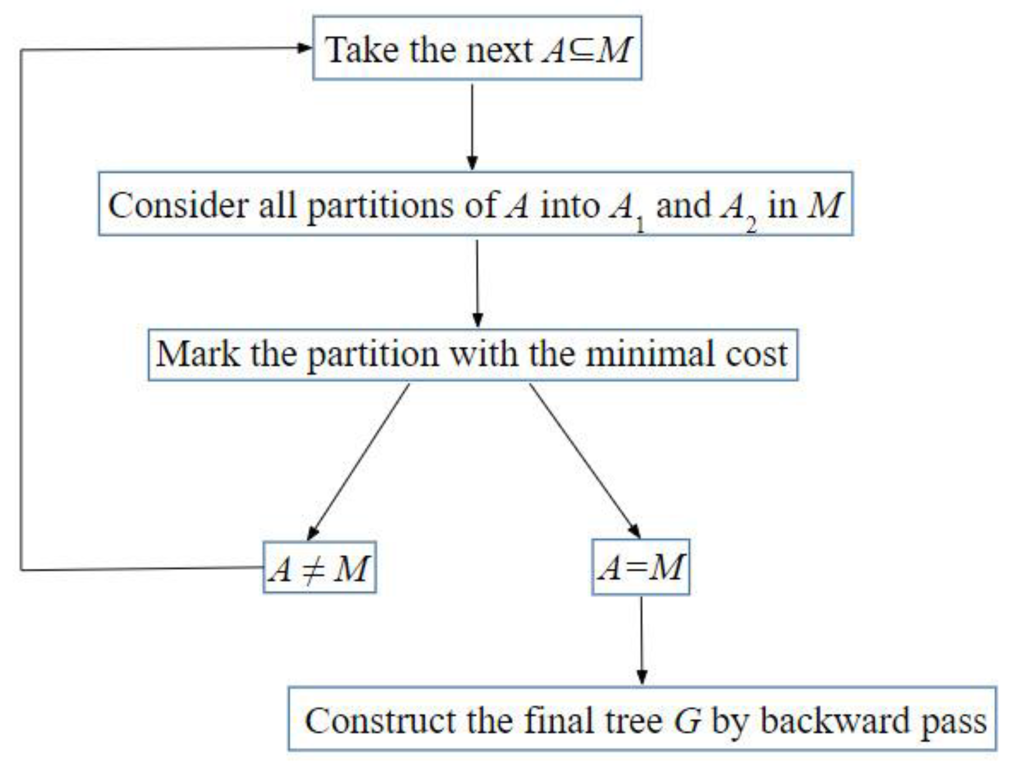
The algorithm presented below exhaustively examines all partitions of each set A = (A1A2) ∈ B, AM. More precisely, we exhaustively examine all pairs consisting of a set AB and a pipe zS, where s2(A) ⊆ z<. For that, we use the following order on pairs (A,z): ascending order of the cardinality |A| of A; for equal cardinalities, we arbitrarily fix an order on the first coordinate; for a fixed A, we fix any order extending the relation < over pipes zS from leaves to the root. According to this order, the algorithm constructs a final tree G = G(A,z) with leaf set A, partition A = (A1A2), and root edge t in G which starts in z. The algorithm constructs a tree G so that A1 = t1< and A2 = t2<, where t1 and t2 are children of the edge t. The algorithm also calculates C(A,z), the sum of costs of embeddings into G over all subtrees in P with root edges eE(A) plus the cost of the minimum embedding of G itself into the subnetwork Sz. This whole sum will be called the cost C(A,z) of the tree G(A,z). Clearly, the tree G* = G(M,r) obtained at the output of the algorithm is a solution to the intermediate tree problem, and its cost equals C(M,r). The flow chart of the algorithm is shown in Figure 8.
The induction base for a one-element set {m} = A and a leaf pipe zS, the tree G(A,z) consists of m and the root edge in m, then C(A,z) = c d p · x E ( A ) ( | x < | 1 ) .
Consider the induction step. It includes four cases, in which T denotes a candidate for G(A,z) and C denotes a candidate for the cost C(A,z). In Cases 1 and 2 below, zS forks in pipes z1 and z2, and in Case 2 it can also be a leaf in S.
If S is a tree, Case 4 is impossible, so only one of Cases 1–3 can be applied. Moreover, if s2(A) ⊆ t1<, then we may only proceed with Case 1; if s2(A1) ⊆ t1<, s2(A2) ⊆ t2<, we may only proceed with Case 3; if none of these conditions is satisfied, we proceed with Case 2. However, below we present the general algorithm assuming S to be a network.
(1) Let zS be a tree-type node (a hybrid node is considered in Case 4), and assume that an edge tG leaves z and enters the pipe z1, i.e., s2′(t) ≤ z1. This is the case of a loss of edge t at node z with respect to the embedding s2′. Let T = G(A,z1) and C = (A,z1) + l, where l = elm if z2< contains an element from s2(M) and l = ilm otherwise. Note that A = t< and that for the tree S, the relation s2(A) ⊆ z1< holds in this case only. Symmetrically for t2.
(2) Let A1,A2B be a partition of A, and assume that there is duplication in a pipe zS with respect to s2′, i.e., s2′(t) = zS and the edge t is forked in z into t1 and t2. Let T = G(A1,z)^G(A2,z), where ^ denotes the union of trees G(A1,z) and G(A2,z) under a common root, i.e., t1< = A1 and t2< = A2. Denote by k the number of nodes vP, such that s1′(v) = t, i.e., one edge leaving v lies in E(A1) and the other is in E(A2). Let
C = C(A1,z) + C(A2,z) + {cdm + cdp·(|E(A1)| + |E(A2)| − |E(A)| − k) + elp·(|E(A1)| + |E(A2)| − 2k)}
If s1(P0) intersects with both A1 and A2, or C = C(A1,z) + C(A2,z) + {cdm + ilp·|E(A)|} otherwise.
(3) Let A1,A2B be a partition of A and assume that s2′(t) = z, i.e., the edge t is forked at a furcation zS, z1 is entered by edge t1 with clade A1, and z2 is entered by edge t2 with clade A2. This is the case of a coordinated furcation of t and z. As in Case 2, let T = G(A1,z1)^G(A2,z2), and let k be the number of nodes vP with s1′(v) = t. Let
C = C(A1,z1) + C(A2,z2) + {cdp·(|E(A1)| + |E(A2)| − |E(A)| − k) + elp·(|E(A1)| + |E(A2)| − 2k)}
If s1(P) intersects with A1 and A2, and C = C(A1,z1) + C(A2,z2) + ilp·|E(A)| otherwise. Note that the condition s2(A1) ⊆ t1< and s2(A2) ⊆ t2< on the tree S holds in this case only.
(4) Edge t leaves a hybrid node z and goes into its unique child pipe z0, i.e., s2′(t) ≤ z0. Then, T = G(A,z0) and C = C(A,z0).
For a final G(A,z) at step (A,z), the algorithm chooses the tree T with the minimum value of C over all cases and all partitions of A. This number C will be the cost C(A,z) of this tree T; at each step (A,z), the algorithm obtains the cost C(A,z) of a final tree G(A,z). For the final output tree, the algorithm chooses G* = G(M,r), where r is the root pipe in S. This G* is a solution to the intermediate tree problem. All these facts are proved below.
Proof of Theorem 1.
The proof is constructed by induction, in the dynamic programming style typically used for the optimization of a loss function, the latter being in our case the cost of the tree G.
The algorithm exactness. Using induction on all pairs (A,z), let us check that for each of the above four cases the cost c(T,A,z) of the tree T specified in this case equals the number C given there. In particular, the cost of the final tree G* = G(M,r) is C(M,r). The induction base, as well as induction steps of Cases 1 and 4, are obvious. Consider Case 3 of the algorithm; Case 2 is considered similarly. Recall that c(T,A,z) = c(s1′) + c(s2′), where c(s1′) is the total cost of embeddings into T of subtrees in P with root edges from E(A) (we call it the first part of the cost) and c(s2′) is the cost of the embedding of T into Sz (the second part of the cost); denote c(T,A,z) = 1(T,A,z) + 2(T,A,z). In Case 3, we obtain 1(T,A,z) = 1(T1,A1,z1) + 1(T2,A2,z2) + d, where T1 and T2 are subtrees with root edges t1 and t2, and d is the total cost of duplications in t and losses in t_ for the embedding of subtrees from P into T. Similarly, 2(T,A,z) = 2(T1,A1,z1) + 2(T2,A2,z2). Hence, c(T,A,z) = c(T1,A1,z1) + c(T2,A2,z2) + d. By the induction hypothesis, C(A1,z1) = c(T1,A1,z1) and C(A2,z2) = c(T2,A2,z2). It remains to show that {…} = d, where {…} is the third term in the expression for C. Indeed, the edge t is entered by |E(A)| edges from P, and the edges t1 and t2 are entered, respectively, by |E(A1)| and |E(A2)| edges that are children of the edges entering t. From the subtrees with root edges in E(A), delete everything that is below the edges entering t1 or t2. We obtain |E(A)| trees, in total with |E(A1)| + |E(A2)| leaves. Let I be the set of inner nodes in them. Clearly, |I| = |E(A1)| + |E(A2)| − |E(A)|. Every node in I is either a duplication in t or a furcation in t_, and vice versa, any such duplication or furcation corresponds to a node in I. By the definition, the number of furcations is k, and all other nodes in I are duplications. Among the |E(A1)| + |E(A2)| edges entering t1 or t2, exactly 2k do not generate a loss in t. Losses in t are either all explicit or all implicit, which depends on the sets A1 = t1< and A2 = t2< only. In the first case, we obtain the first expression for C. In the second case, we have k = 0, which implies that there are no duplications in t; i.e., |E(A1)| + |E(A2)| = |E(A)|. This follows from the facts that P and G are trees and from the definition of s′.
Now, following the same induction, we prove that the cost C(A,z) of the tree G(A,z) constructed at step (A,z) is the desired minimum in the intermediate tree problem. Let X be a minimum tree with leaf set A; by the condition, all its clades belong to some B which with respect to P, Sz, and some embedding s2: XtSz is minimal in the intermediate tree cost; in particular, s2: XtSz is a minimum embedding. For X, the conditions of one of Cases 1–4 of the algorithm are satisfied. Let, for example, the conditions of Case 3 be fulfilled; the other cases are considered similarly. Denote by f(X) = s1′(X) + s2′(X) the minimized cost in the intermediate tree problem. Denote by X1 and X2 the subtrees with root edges t1 and t2 embedded in the subnetworks Sz1 and Sz2. Their clades are some sets A1 and A2 in B. Repeating the arguments of the preceding paragraph, we obtain f(X) = f(X1) + f(X2) + d, where d is the sum of duplications in t in losses in t_ when embedding the subtrees from P into X. Then, we have
C(A,z) ≤ C(A1A2, z) = C(A1,z1) + C(A2,z2) + df(X1) + f(X2) +d = f(X);
here, C(A1A2, z) is the value of C computed with respect to the partition A1 and A2. Hence, f(G(A,z)) = f(X).
The algorithm runtime. We construct sets E(A) for all AB in a time of the order of |B|·|P|. Inclusions and intersections for sets in B are computed in a time of the order of |B|2 ·|M|. Inclusions of sets from B into clades of the network S are computed in a time of the order of |B|·|S|·|M|. All partitions of each set AB into sets A1,A2B are computed in a time of the order of |B|3; for every triple A, A1, A2 of sets one checks that A1 and A2 are disjoint and |A1| + |A2| = |A|. For every AB and every partition into A1 and A2, one computes the number k of nodes vP in a time of the order of |P|. The number of sets A and of partitions of A is no greater than |B|, so the total computation time for all k and for all A is of the order of |B|2 ·|P|.
At each induction step when constructing the trees G(A,z), for each AB and each pipe t we examine at most |B| partitions of A. For each partition, the cost C is computed in a constant time. Therefore, the total construction time for all G(A,z) is of the order of |B|2·|S|. The total runtime of the algorithm is at most of the order of |B|·(|B|·|M| + |S|·|M| + |B|2 + |B|·|P| + |B|·|S|). □
Remark 1.
If S is a tree, then the described algorithm can be generalized so that to take into account horizontal transfers when computing the embedding of G into S. Such an event assumes that pipes in S are divided into time layers, which often results in occurrence of nodes of degree 2 (see [22]). A horizontal transfer consists of transferring an edge of G from one pipe of S into another pipe lying in the same time layer. A transfer may have a furcation at the source or do not have it (in the first case, the furcation occurs in the pipe, with one of the child edges remaining in its pipe and the other being transferred). To obtain the corresponding algorithm, we need to add two more cases to the described-above algorithm. These are furcation of an edge e in z with transferring one of the child edges to another pipe in the same time layer, and transferring an edge e (without furcation) to another pipe of the same layer. In both cases, it is not necessarily required that s2(A) ⊆ z<.

2.5. Constructing the Main Parameter of the Algorithm

Recall that M is a set of leaves in a tree G* to be constructed by the algorithm from Section 2.4 (Theorem 1). The sought-for intermediate tree G* depends on a fixed collection B of subsets in M; this B is called the main parameter of the algorithm. Since the intermediate tree problem is NP-hard, any polynomial-complexity algorithm does not necessarily find an intermediate tree G** with an absolutely minimum cost which is a solution of the original problem in the unconditional setting (if PNP).
Given an arbitrary collection B′ of subsets of M, the main parameter is a collection B satisfying property (*), whose construction is described in Appendix A; this B contains, at most, |M| times as many elements as the original B′.
Let us extend a given B′ by adding images (under s1) of all clades in P and inverse images (under s2) of all clades in S; then we pass to B using the procedure described in Appendix A. Nevertheless, execution of the algorithm from Section 2.4 with this collection B may produce a result G* whose cost can sometimes be essentially greater than the cost of the tree G**.
Let us present a further extension for collection B′, which could be of use in applied computations. We first describe this extension for the case where S is a tree. Consider the trees P and S with their embedding composition s2(s1)′. For each pipe zS, one considers the set Oz of edges in P that leave z. For each subset O′ ⊆ OzP, one adds to B′ all images s1(∪{e<|eO′}) for all O′ ⊆ Oz and all zS and then extends the obtained B′ to the main parameter B. Simulation has shown that for such B runtime of the algorithm from Section 2.4 remains to be cubic but the cost C* of the tree G* reduces significantly, so that C* becomes close to the solution of the unconditional problem (simulation results are not presented here).
If, nevertheless, the main parameter B is not sufficiently large to provide a smaller C*, we may use another mapping of P to S, which provides the minimum of duplication clusters (the definition and an efficient construction algorithm for this mapping are described in [23]). For example, the two bottom duplications in Figure 2b form a cluster in the sense of [23]. That embedding differs from our embedding s′ in that duplications often occur higher than under s′, which leads to increasing cardinalities of the sets Ot. If a main parameter B slows down the execution of the algorithm too much, we may, vice versa, consider the tree S with time layers, which reduces the sets Ot; in this case, the definition of the embedding and an efficient construction algorithm for it are described in [22].
If S is a network, then the extension of a standard collection B0 is defined via the embedding s′: PS constructed in Theorem 3 disregarding ILS events. Let us briefly recall the construction. Exhaustively examine all pairs consisting of an edge eP and a pipe zS with condition s2(s1)(e<) ⊆ z<. For each such pair (e,z), one constructs a minimum embedding of the subtree Pe into a subnetwork Sz inductively; when passing to a larger pair (e,z), one chooses the case in Section 2.4 with the smallest cost. The resulting embedding is a mapping from P = Pr to the network S = Sr, where r′ and r are the root edge and the root pipe in P and in S.
One can also adjust collection B using an embedding which, along with duplications and losses, takes account of Incomplete Linear Sorting events (see Section 2.7 below).

2.6. Example of the Algorithm Operation

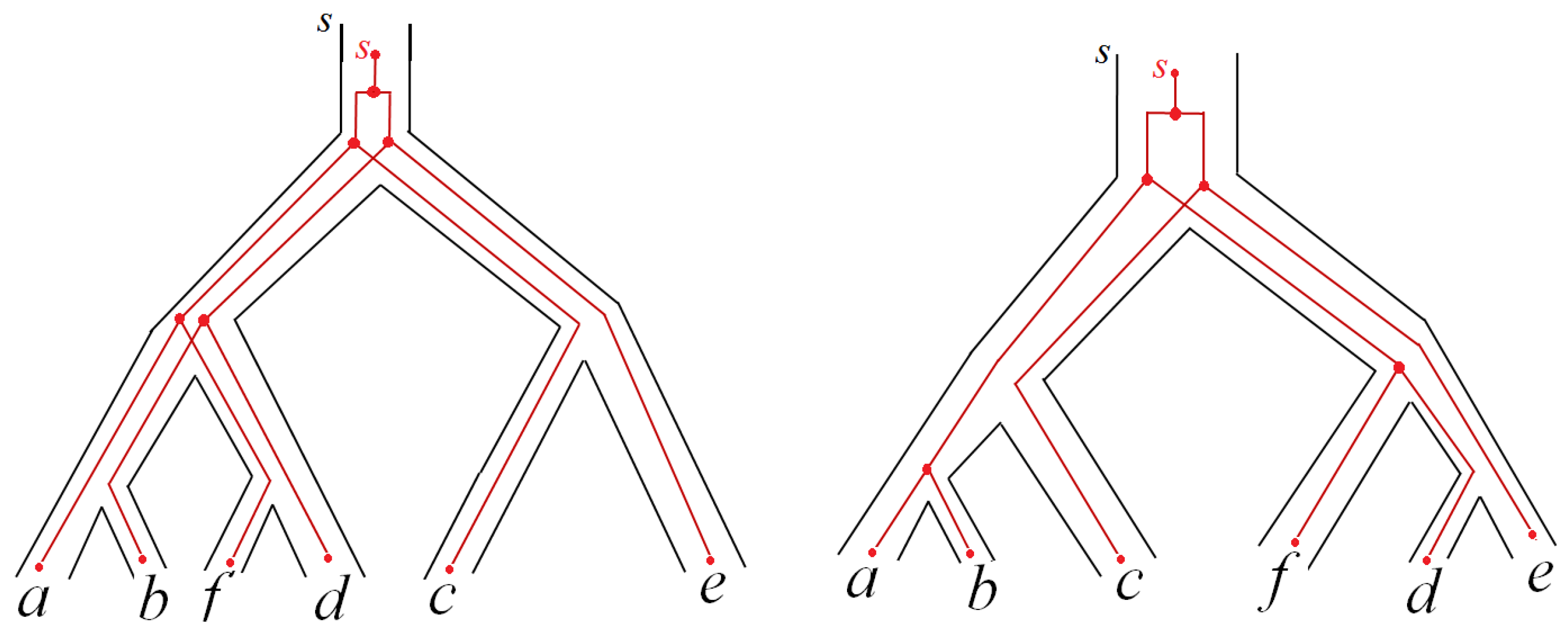
Let us show how the algorithm works using an example from [6], where S = (((a,b),c),(f,(d,e))) is a tree, P = (((a,f),c),(e,(b,d))), M = {a,b,c,d,e,f}; and s1 and s2 map each leaf to itself. Let the cost of all explicit losses be 2, of all implicit losses be 1, and of all duplications be 3; and collection B′ is as follows: {a,f}, {a,f,c}, {b,d}, {e,b,d}, {a,b}, {a,b,c}, {d,e}, {f,d,e}, the set M itself, and all one-element sets in M. The embedding s′: PS is shown as an image tree in Figure 9.
Construct the main parameter B. The root pipe adds to B′ the sets {a,b,f,d}, {a,f,e}, {b,c,d}, {c,e}, {a,b,c,f,d}, {a,c,f,e}, {a,b,d,e}, and {b,c,d,e}. The left-hand child pipe adds to it the sets {a,c} and {b,c}, and the righ-hand one adds {f,d} and {f,e}. Clearly, B satisfies condition (*).
Construct trees G(A,z) for all sets AB, zS, z being the ancestor edge for the set A of leaves. For one-element and two-element sets A, the trees are trivial. Consider three-element sets A. For the set A = {a,f,c}, the trees ((a,f),c) and ((a,c),f) have the same cost. For {e,b,d}, the tree (b,(d,e)) is the one of the minimum cost among the two trees. For {a,b,c} and {f,d,e}, the trees ((a,b),c) and (f,(d,e)) are those of the minimum costs among the three trees. For {a,f,e} and {b,c,d}, the trees (a,(f,e)) and ((b,c),d) are those of the minimum costs among the two trees.
For the set {a,b,f,d} in B, the minimum cost is given by the partition into {a,b} and {f,d}; for {a,c,f,e}, by the partition into {a,c} and {f,e}; for {a,b,d,e} and {b,c,d,e}, by the partitions into {a,b} and {d,e} and into {b,c} and {d,e}, respectively.
For the set {a,b,c,f,d} in B, the minimum cost is given by the partition into {a,b,f,d} and {c}. Finally, for the whole M, the minimum cost is given by {a,b,f,d} and {c,e}. Thus, the resulting tree G* is (((a,b),(f,d)),(c,e)), the resulting cost C* = 26, and the obtained embeddings s1′: PG and s2′: GS are shown in Figure 10. In total, they contain 2 duplications and 11 losses. This is the global minimum G** of the cost of a tree G in the unconditional problem.
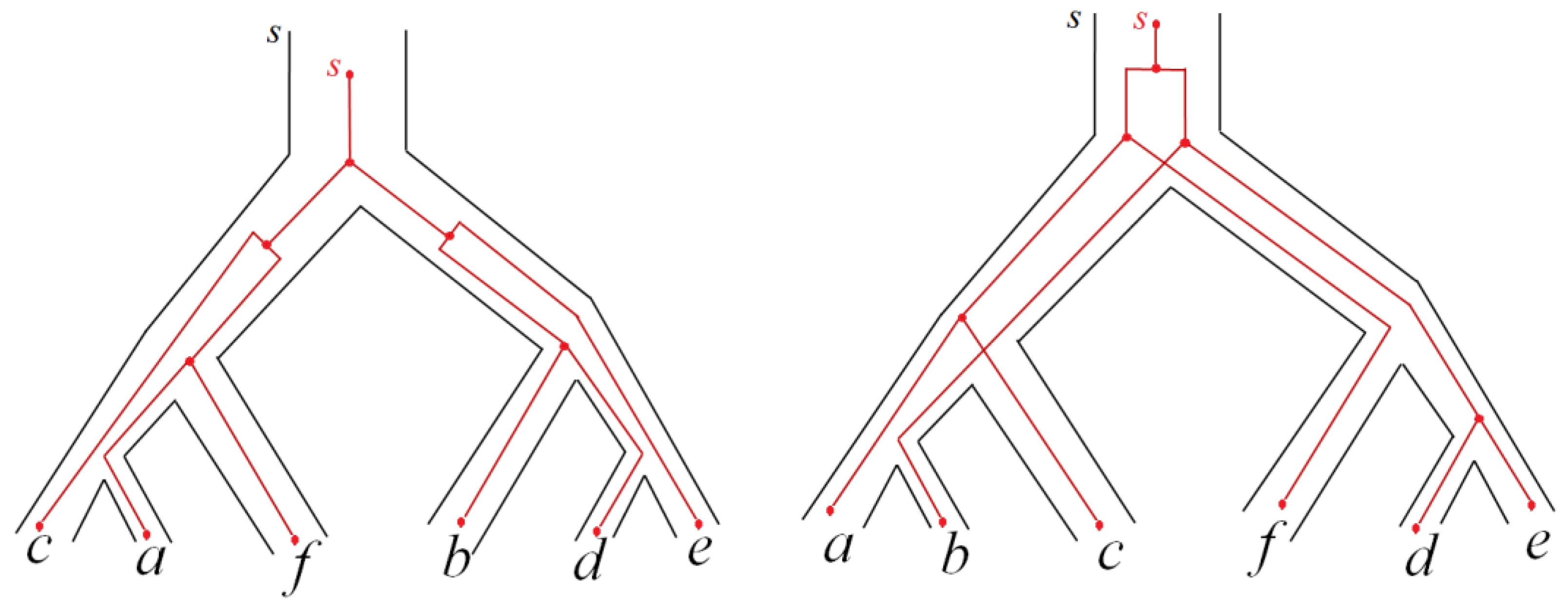
For all costs equal to 1, our algorithm outputs the same tree G*. For the same input data, the algorithm from [8] has constructed the tree G = (((c,a),f),(b,(d,e))); the corresponding embeddings are shown in Figure 11. Here, in total, there are 3 duplications and 11 losses.
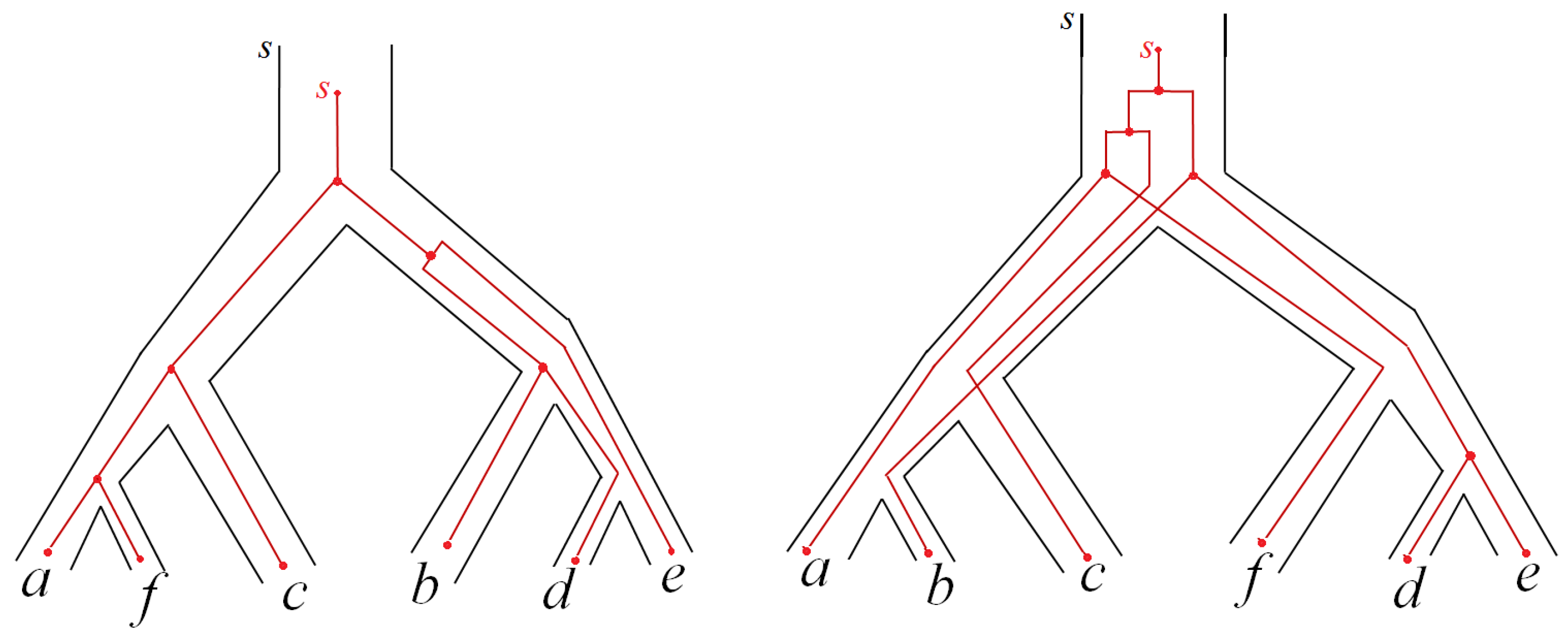
If we confine ourselves with the main parameter B′, our algorithm constructs a tree with a cost strictly greater than in the unconditional problem; namely, 3 duplications and 11 losses (see Figure 12). In [8], there are also 3 duplications and 11 losses, but our embeddings are quite different (see Figure 11 and Figure 12).

2.7. ILS-Minimum Embedding of a Tree into a Network and Theorem 3

Let G and S be any given binary tree and binary network, respectively, and let s″: G → S be an embedding. The Incomplete Linear Sorting (ILS) event is an edge eG entering a pipe tS provided that at least two edges enter t (see [9]). The locus of an ILS event is the pipe t. The ILS-cost over a pipe tS entered by kt ≥ 1 edges from G is defined as ct = c·(kt –1), where c is the cost of a single ILS plus the costs of all duplications and all losses in t. The ILS-cost over S is defined as t S c t plus the costs of all duplications and all losses in S, where t runs over pipes tS entered by at least one edge from G; the latter is denoted as tS↓. Such pipes will be called non-empty, while all others are said to be empty. Clearly, t B c t = c ( t B k t n ) , where n is the number of non-empty pipes in S.
An ILS-minimum embedding of s′: GS is defined to be an embedding with the total minimum cost of c ( t B k t n ) , where n is the number of non-empty pipes in s′, plus the costs of all duplications and losses. This cost is called the ILS-minimum cost of s′; it reflects how much s′ differs from an isomorphism.
Similarly, we define an ILS event for a given set {se: GeS} of embeddings of different trees Ge into a given network S. Edges occurring in S from different se are considered equally. The ILS-cost of a set {se} is defined by the same expression c ( t B k t n ) , where n is the number of pipes that are non-empty for at least one of the embeddings se, plus the costs of all duplications and all losses in S. A set {se} is called an ILS-minimum set of embeddings if the ILS-cost of {se} is minimal as compared to any set {re: GeS} of embeddings of these Ge into S with some conditions on all se and re. This cost is called the ILS-minimum cost of {se}.
A bridge in S is a pipe t for which any path from the super-root to the clade t< contains t. In our case, this is equivalent to the following condition: t is a pipe such that its removal makes the undirected graph corresponding to S disconnected. A leaf pipe is always a bridge. A block in S is an inclusion-maximal set of nodes in S for which the induced subgraph does not contain a bridge. Two blocks either coincide or are disjoint. For example, in Figure 6, bridges are the pipe u7-u6 and also the root and leaf pipes; blocks are the super-root, leaves, and two complements to the edge u7-u6 without the root or leaf pipes. Note that blocks of a network S form a rooted, though now non-binary, tree. For a network S of level k any block contains at most k hybrid nodes. This number k is a measure of distantness between S and the tree.
We say that pipe t enters block B if B contains its head t but does not contain its tail t+; such a t is unique for B and is a bridge in S. Pipe t leaves B if B contains its tail t+ but does not contain its head t; there can be many pipes leaving B, and all of them are bridges in S. In what follows, for any pipe tS we assume a unique block Bt in S, such that tB; however, we consider the embedding GeSt. The mapping tBt between incoming pipes t and blocks B in S (except for the super-root) is a one-to-one mapping.
For an arbitrary non-empty set A of leaves in an arbitrary network S, E(A) is defined exactly as in the above case where S is a tree. Namely, for an edge eG the relation eE(A) means the following: s(e<) ⊆ A and there is no e1G for which e1 > e and s(e1<) ⊆ A. It is easily seen that for any edge e entering a pipe tS we have eE(t<) or ∃e′ > e (e′ ∈ E(t<)). As is noted above, if S is a tree, then finally there remains only one disjunction term eE(t<).
Let s″: GS be an embedding, and introduce the following condition:
(*) each non-root pipe t which is a bridge in S is entered by precisely edges from E(t<).
We have proved the following result.
Theorem 3.
Let s: G0 → S0 be an arbitrary mapping from leaves of a binary tree G to leaves of a binary network S. The algorithm has been constructed which outputs an ILS-minimum continuation s′: G → S of s with the property (*). Its runtime is of the order of |G|·|S|·k·24k, where |·| is the number of nodes in the tree or network and k is the level of the network S. It is exact if the cost of a single ILS is not less than the sum of the duplication cost and the cost of an implicit loss.
In [9], a construction algorithm was suggested for a minimum (with respect to ILS events only) embedding of a tree into a network of level 1. Additionally, in [9] (section “Conclusion”), a method was outlined to generalize that algorithm to the case of a network of any level k. Our algorithm uses the idea from [9] combined with ideas of the algorithm of Theorem 1.
Denote by cd, el, il, and ci, respectively, the costs of duplication, explicit loss, implicit loss, and ILS event.
Claim 1.
If ci ≤ cd + el, then there exists an ILS-minimum embedding s*: G → S such that property (*) is valid.
Proof. 
Let s′ be any ILS-minimum embedding. We successively rearrange s′ to a desired embedding s*; to this end, we exhaustively examine all non-root bridges tS in an arbitrary order. The algorithm that we will construct now is not used in what follows; i.e., we need Claim 1 as an existence result only. Namely, in the Proof of Theorem 3 we construct an embedding s′: G → S, which possesses property (*) and is minimal among the embeddings with property (*); considering Claim 1, it will be absolutely minimal.
We perform the proof by contradiction. Assume that tS and we have the following:
(**) edge e1G enters t, e1E(t<), and e1 is an edge the most distant from the root among edges satisfying these two conditions.
Let us show that a sibling edge e2 of e1 also satisfies all the three conditions, and rearrange s′ so that again to obtain a minimum embedding s″ such that both e1 and e2 do not enter t, there arises one new edge entering t, and the number of edges entering all other pipes does not increase. We repeat this rearrangement until we find an edge e1 satisfying condition (**).
Thus, take e′ > e1 (e′ ∈ E(t<); such an e′ is unique. Consider a path φ from the root through the edges e′ and e2 to some leaf and a path ψ of pipes that contain φ so that ψ ends at t<. Then, ψ passes through t. Assume that some edge e3 in φ enters t. Then, we must have e3 = e2. Indeed, by the choice of e1, the edge e3 on φ cannot lie below e2, and since e1 enters t, it cannot lie above e2. Thus, e1 and e2 enter t and are forking from some edge e, i.e., they fork at eG. Let z = s′(e).
If z is a pipe, then e1 and e2 appeared in z as a result of a duplication and entered child pipes of z, either both entered the same pipe z1 or each one entered its own. In the first case, the duplication can be moved to z1, child of z, thus reducing the numbers of losses and ILS events when computing the embedding cost of s′; in the second case, the duplication can be eliminated by moving it to z. In both cases, the cost of the resulting new embedding becomes strictly less, which contradicts the minimality of s′. The case that z is a hybrid node is impossible.
If z is a tree-type node, then the edges e1 and e2 arise in z and are continued to t. Consider a new embedding s″, which differs from s′ only by the fact that s″(e) = t, and draw a path pe along any of the paths pe1 or pe2 (see Figure 13).
For s″, one explicit loss appears at z. In the node t+, one ILS event is replaced with a duplication at t and loss at z. The embedding cost does not increase, but now the number of edges e entering t is less by 1, and the number of edges entering any other pipe have not increased. By repeating this modification, we find the desired ILS-minimum embedding s*.
Let a set D of hybrid pipes in a network S be fixed. For an embedding s″: Ge → St of a subtree G with root edge e into a subnetwork of S with root pipe t, a block BtS is said to be D-coordinated if D is the set of non-empty hybrid pipes in B. For the same embedding s″, denote by N(t,D) the set of all non-empty pipes in Bt. The cardinality of this set will play an important role in what follows.
For a set M = {GeSt: eX} of embeddings of subtrees into a fixed subnetwork, where X is a fixed set of edges of G, a block BtS is said to be D-coordinated if D is the set of hybrid pipes in Bt that are non-empty for at least one embedding in M.
Claim 2.
Let e ∈ G, t ∈ S and Bt be a block in S with t ∈ Bt. We construct an algorithm which, given any leaf mapping s: Ge → St and any set D of hybrid pipes in a block Bt ⊂ S, outputs a set Y, such that Y = N(t,D) if there exists a continuation s″: Ge → St of s that D-coordinates Bt. The runtime of the algorithm is if the order of |Bt|.
Proof. 
Let such an s″ exist. The algorithm exhaustively examines bridges that leave Bt and records which of them are empty. For that, we use the fact that a bridge x leaving Bt is empty with respect to s″ if, and only if, the clade of x is disjoint with s″(e<). Then, the algorithm exhaustively examines tree-type pipes xBt from leaves to the root and labels x as empty, if and only if, either x = t or both child pipes of x are empty; labels of hybrid pipes are known by the condition.
For any embedding of leaves s0: G0 → S0, we delete from S the subnetwork of every pipe, such that its clade is disjointed with s0(G0) and its sibling clade is not. In the resulting graph S′, we combine maximum-length sequences t1 > … > tn of pipes (ti+1 is a child pipe to ti) in S for each of which (for 1 ≤ in − 1) one child subnetwork has been deleted into a «compound» pipe t, which will be referred to as new; we again denote the resulting binary network by S′. For every new pipe in S′, denote l(t) = n ≥ 2; for all other pipes in S′, denote l(t) = 1. The leaf mappings s0: G0 → S0 and s0: G0 → S0′ coincide.
For a binary network S′, we formulate a new minimum embedding problem. We replace the search for a minimum embedding s′: G → S with the search for a minimum embedding s′: G → S′. The latter is more convenient due to the fact that for every tree pipe tS′ there are edges e1 and e2 that enter, respectively, the child pipes t1 and t2. Furthermore, the cardinality of the network S′ is not greater (and typically less) than the cardinality of S.
Thus, we define an implicit loss in S′ to be a pair (e,t) where the edge e enters a new pipe tS′; if a new pipe is the root pipe rS′, then e is the root edge in G. Therefore, to several implicit losses in the former sense there corresponds a single implicit loss in the new sense. The cost of a new implicit loss is set to be il ·(l(t) − 1), where il is the cost of a single implicit loss equal to its former value. The locus of an implicit loss is assumed to be the pipe t. An explicit loss and a duplication are defined as above and have the original costs el and ed. An ILS event is defined as above; it is a pipe entered by strictly greater than one edge. However, the cost of a new ILS event on a pipe t is ci·(kt − 1)·l(t), where kt is the number of edges entering t. We split this cost into a sum of two terms, the first ILS term and the second ILS term, ci·(kt − 1) and ci·(kt − 1)·(l(t) − 1). The cost of a new ILS event on a network S is c i ( t k t n ) + c i ( t ( k t 1 ) ( l ( t ) 1 ) ) , where kt  1 and where n is the number of non-empty pipes in S′. Here, we will also distinguish between the first ILS term and the second ILS term. The ILS-minimum continuation and the ILS-minimum cost are defined as above, taking into account all the above-mentioned events. Thus, the new problem is to find an ILS-minimum continuation s: G → S′ of s0 with property (*). This problem is of interest in connection with the following fact.
Claim 3.
Given a solution of the new problem by a linear-time algorithm, one can construct a solution of the original problem with property (*).
Proof. 
Let s′: G → S′ be a solution of the new problem for a new network S′, and let its ILS-minimum cost be c. Define an embedding s: G → S for the original problem by keeping the values s(g) = s′(g) for all s′(g) except for s′(g) = t, where t is the new pipe in S′. In the latter case, we have s(g) = tn, where tnS is the lowermost pipe in tS′. The ILS cost of s is also c. Assume that there exists a solution s*: G → S of the original problem with an ILS-minimum cost c′ < c. Then, define an embedding s**: G → S′ by keeping the values s**(g) = s*(g) for all s*(g) except for s*(g) = ti, where ti is a part of the new pipe t. In the latter case, we have s**(g) = t. However, the ILS costs of s* and s** are the same. Let us check property (*) for s. Consider edges entering pipe t with respect to s′; with respect to s, they enter either t (if t is not new) or t1, t2, …, tn (otherwise). Since E(t<) = E(t1<) = … = E(tn<), we conclude that any bridge tS is entered by exactly the edges from E(t<).
We again denote the resulting network by S; its size is of the order of |G|, where k is the level of the original (or equivalently, of the resulting) network.
For a given embedding s″: Ge → St, define the B-cost of a block B to be the total cost of all events in B plus the cost of duplications and implicit losses in the pipe t. For a given set {se: Ge → St} of embeddings, let the B-cost of a block B be the total cost of all events in B plus the cost of all duplications and implicit losses in t that arise from all these embeddings se.
For an arbitrary set D of hybrid pipes in Bt, by a D-minimum embedding we call an embedding s″: Ge → St satisfying property (*), with D coordinating the block Bt, and having the smallest Bt-cost among all embeddings Ge → St that satisfy these two conditions. We denote such an s″ by s(e,t,D) and denote its Bt-cost by C(e,t,D). If there is no any such s″, we say that a D-minimum embedding is not defined.
For a set {Ge|eE(t<)}, by a D-minimum set of embeddings we call a set {se: Ge → St} of embeddings satisfying property (*), with D coordinating the block Bt, and having the smallest Bt-cost among all sets {re} that satisfy these two conditions. We denote this Bt-cost by c(t,D) and denote this D-minimum set by s(t,D).
Denote by c(t) the minimum of c(t,D) over all D specified above, which is attained at some D0, and define s(t) = s(t,D0). If |Bt| = 1, then D = ∅. If t is a bridge, then s(t) is called a bridge set, and its elements are referred to as bridge embeddings.
The result of Theorem 3 consists of constructing a set s(r) with r a root pipe in S such that s(r) consists of a single embedding, which is the desired ILS-minimum continuation s′: G → S.
Algorithm for ILS-minimum embedding of a tree G into a network S. By induction, during a forward pass of the algorithm we construct C(e,t,D), and during its backward pass we could construct s(e,t,D), though the latter is not needed. The usual linear order on these pairs is fixed: pipes t from the leaves to the root, and for each fixed t we look through edges e from the leaves to the root.
For each pair (e,t), with properties s(e<) ⊆ t< (if t is not a bridge) or eE(t<) (otherwise), and for each set D of hybrid pipes in Bt, we find a D-minimum embedding s(e,t,D) of Ge → St and its Bt-cost, or notice that they are undefined. We denoted this Bt-cost by C(e,t,D), and for this embedding, denote the set of non-empty pipes in Bt by N(e,t,D). Additionally, for each pair (e,t) we compose a list D(e,t) of admissible sets D.
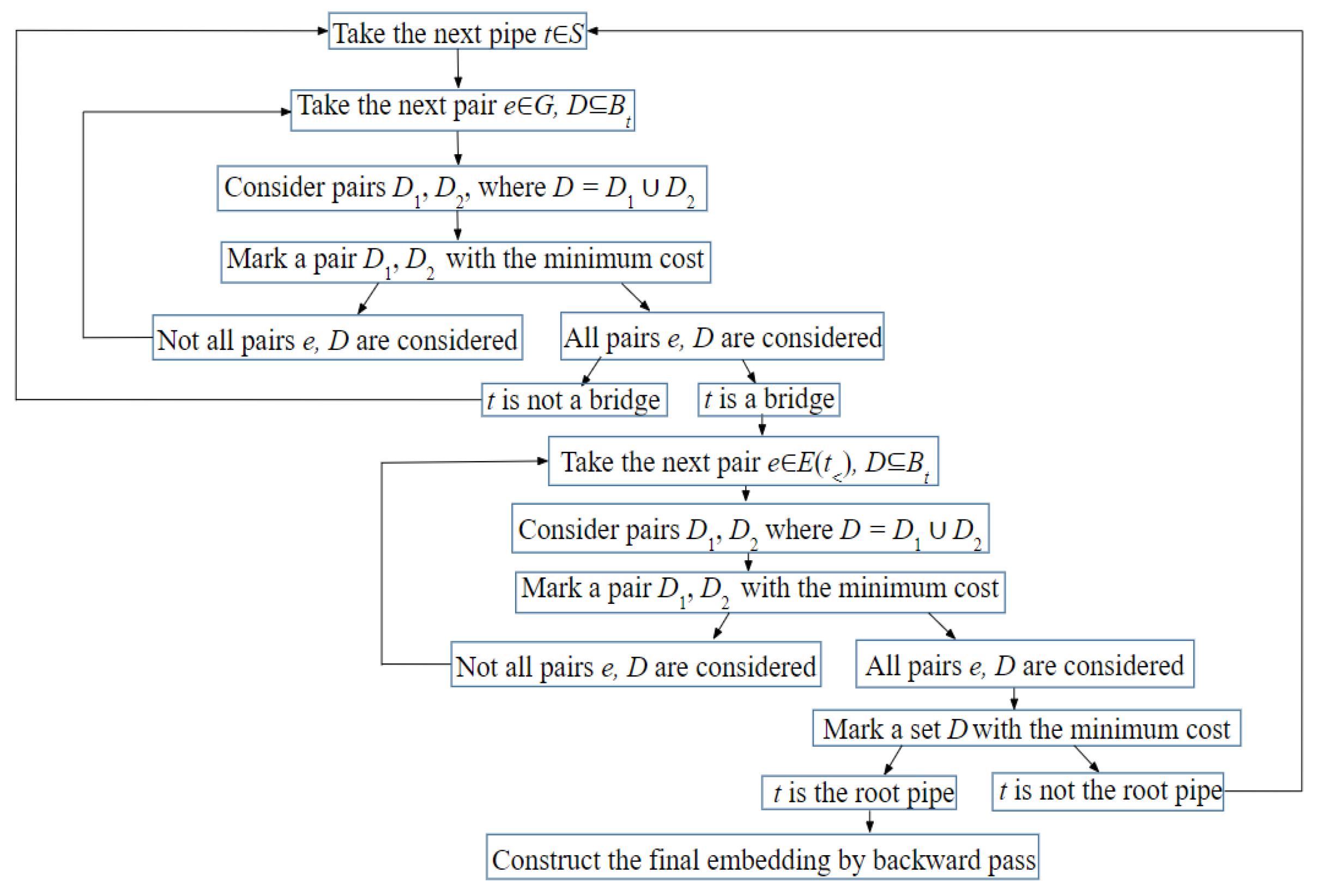
For an arbitrary set M of pipes, define f ( M ) = t M l ( t ) . By Claim 2, the set N(t,D) can be constructed an algorithm which is linear in |S| given the set D; this allows, for any tS and for any sets D1 and D2, to compute in time of the order of|S|2·24k the values of f(N(t,D1) ∩ N(t,D2)) and f(N(t1,D1) ∩ N(t2,D2)), where t1 and t2 are children of t. It is specifically these intersections that are used in what follows. The flow chart of the algorithm is shown in Figure 14.
The induction base for constructing D-minimum embedding and bridge embedding of Ge → St: for a leaf pipe tBt and a leaf edge eG, D(e,t) = {∅} and the embeddings are trivial, its B-cost being C(e,t,D) = il·(l(t)–1).
The induction step for D-minimum embeddings. Consider the following four cases, analogous to those considered in Section 2.4, where U(e,t,D), by the proof given below, will be found to be equal to the B-costs of the embeddings defined below. In Cases 1–4 below, computations are performed if all the involved quantities are well defined and all the required conditions are fulfilled. Recall that D is a set of hybrid pipes in B.
(1)
Assume that edge e leaves t and “swings” to the child pipe t1 at a furcation in S, and t1D (if t1 is a hybrid pipe) or eE(t1<), D = ∅ (if t1 is a bridge) or D is arbitrary (if t1 is a tree-type pipe and is not a bridge). The embedding continues (since e+t) an already known (D\t1)-minimum (if t1 is not a bridge) or bridge (otherwise) embeddings of GeSt1. Its B-cost is, respectively, U(e,t,D) = U(e,t1,D\t1) + el + il·(l(t)–1) if D\t1D(e,t1), or U(e,t,D) = el + il ·(l(t)–1), symmetrically for t2. For each e, t, and D, if, in this case or in one of the cases below, we have U(e,t,D) < ∞, then we add D to the list D(e,t).
(2)
Assume edge e forks in t into e1 and e2. Exhaustively examine all pairs (D1,D2) where D1 and D2 are any sets of hybrid pipes in B, such that D1D(e1,t) and D2D(e2,t). For each D′ = D1D2Bt we set the initial value of U(e,t,D′) = ∞. For every (D1,D2) compute
V = U(e1,t,D1) + U(e2,t,D2) + ci·f(N(e1,t,D1) ∩ N(e2,t,D2)) + cd + il ·(l(t) − 1).
If V is strictly less than the current value of U(e,t,D′) for D′ = D1D2, set U(e,t,D′) = V. In particular, we compute U(e,t,D).
(3)
Assume that edge e forks at a furcation in S, t1 is entered by edge e1, and t2 is entered by e2. For each D′ we set the initial value of U(e,t,D′) = ∞. If t1 and t2 are not bridges, exhaustively examine all pairs (D1,D2), where D1 and D2 are sets of hybrid pipes in B, such that D1D(e1,t1), D2D(e2,t2). For every (D1,D2) compute
V = U(e1,t1,D1) + U(e2,t2,D2) + ci·f(N(e1,t1,D1) ∩ N(e2,t2,D2)) + il ·(l(t) − 1).
If V is strictly less than the current value of U(e,t,D′) for D′ = D1D2 ∪ {t1,t2}, set U(e,t,D′) = V. Here, by the definition, the set {t1,t2} contains only hybrid pipes.
If exactly one of the pipes t1 and t2 is a bridge (assume that this is t1), exhaustively examine each sets D2 of hybrid pipes in B such that D2D(e2,t2). For D2, if e1E(t1<) compute V = U(e2,t2,D2) + il ·(l(t) − 1), and if V is strictly less than the current value of U(e,t,D2 ∪ {t2}), set U(e,t,D2 ∪ {t2}) = V. Here, similarly, the set {t2} contains only hybrid pipes.
If both pipes t1 and t2 are bridges, e1E(t1<), and e2E(t2<), set U(e,t,∅) = il ·(l(t) − 1). In particular, we compute U(e,t,D).
(4)
Assume that edge t′ leaves t, enters its unique child pipe t1, and t1D (if t1 is a hybrid pipe); eE(t1<) and D = ∅ (if t1 is a bridge). Then, the embedding continues (since e+t) the already known (D\t1)-minimum (if t1 is not a bridge) or bridge (otherwise) embedding GeSt1, and U(e,t,D) = U(e,t1,D\t1) + il ·(l(t)–1) if D\t1D(e,t1), or U(e,t,D) = il ·(l(t)–1).
Choose an appropriate case that has the minimum B-cost U(e,t,D) and memorize it, as well as the sets D1 and D2 in Cases 2 or 3. These will be used in the further backward pass of the algorithm, which will result in the construction of a s(e,t,D) embeddings. There is no need to compute U(e,t,D) for e, t, and D; these values are needed only for arguments satisfying the given conditions, which are necessary to proceed with the next cases of the algorithm. As is proved below, C(e,t,D) = U(e,t,D); accordingly, the backward pass of the algorithm finds the embeddings s(e,t,D): GeSt.
(5)
The induction step for bridge embeddings after the corresponding construction step for D-minimum embeddings. Let t be a bridge. By property (*) (see the Proof of Theorem 3 below), t is entered by precisely the edges from E(t<). Arbitrarily order edges e1, e2, e3,…,emE(t<). Similarly to what was performed in Case 2 (but without the cd term), by exhaustively examining pairs D1, D2 of sets of hybrid pipes in B, where D1D(e1,t) and D2D(e2,t), for every D = D1D2 we find D1′ and D2′ that correspond to a D-minimum two-element set M2 = {Ge1St, Ge2St} of embeddings. More precisely, for each D we minimize over D1 and D2, where D = D1D2, the quantity V in the expression from Case 2 without the cd term, i.e.,
V = U(e1,t,D1) + U(e2,t,D2) + ci·f(N(e1,t,D1) ∩ N(e2,t,D2)) + il ·(l(t) − 1.
Assume that the minimum of V is finite and is attained at some D1′ and D2′. Denote it by U(e1,e2,t,D) and add D to the list D(e1,e2,t) of admissible sets. Note that the set M2 = {s(e1,t,D1′), s(e2,t,D2′)} itself is not used here. Let D1′ = f21(D) and D2′ = f22(D). Again examining pairs D1, D2, where D1D(e3,t) and D2D(e1,e2,t), for every D = D1D2 we find D1″ and D2″ that correspond to a D-minimum 3-element set M3 = {Ge1St, Ge2St, Ge3St} of embeddings. More precisely, for each D we minimize over D1 and D2, where D = D1D2, the quantity
V = U(e3,t,D1) + U(e1,e2,t,D2) + ci·f(N(e3,t,D1) ∩ N(e1,e2,t,D2)) + il ·(l(t) − 1.
Assume that the minimum is finite and is attained at some D1″ and D2″. Denote it by U(e1,e2,e3,t,D) and add D to the list D(e1,e2,e3,t) of admissible sets. Note that the set M3 = {s(e1,t,f2,1(D1″)), s(e2,t,f2,2(D1″), s(e3,t,D2″)} itself is note used here. Proceeding further in this way with computing U(e1,e2,…ei,t,D), for each D we construct a D-minimum set Mm = {Ge1St, Ge2St,…,GemSt} of embeddings, which we denote by s(t,D). The set s(t,D) contains exactly m = |E(t<)| embeddings, where m is the number of edges entering t.
Choose a bridge set s(t) = s(t,D0) with the minimum U(e1,e2,…em,t,D) over all D. For t = r, the root pipe, this set s(r) consists of a single element, which is the desired embedding s′: GS with the minimum B-cost. The ILS-minimum cost s′ equals the sum over all bridges tS of Bt-costs of sets s(t) plus the costs of ILS events in t, where Bt corresponds to t.
Proof of Theorem 3.
To prove the exactness of the algorithm, we first show that the expressions for computing U(e,t,D) in the algorithm output the Bt-cost of the corresponding embeddings, which, clearly, D-coordinate the block Bt. For Cases 1 and 4, note the following, the embedding GeSt, as compared to the embedding GeSt1, has one non-empty pipe (t1) more and one entry (into t1) more. Therefore, the first ILS term is the same for both embeddings. This is also true for the second ILS term as well, since it equals 0 at t. For Case 3, the embedding GeSt, as compared to the union of embeddings Ge1St1 and Ge2St2 has two non-empty pipes (t1 and t2) more and two entries (into t1 and t2) more. Therefore, the first ILS term of the embedding GeSt and of the union Ge1St1 and Ge2St2 are the same if pipes that are non-empty for both embeddings of the union are counted once each time. Similarly, the second ILS term of the embedding GeSt and of the union are the same if pipes that are non-empty for the embeddings are counted l(t)−1 times. This explains the presence of the term ci·f(N(e1,t1,D1) ∩ N(e2,t2,D2)) or, in Case 2, ci·f(N(e1,t,D1) ∩ N(e2,t,D2)) in the expressions for C. Additionally, for Case 2 let us check that in the expression for V we may use the values U(e1,t,D1) = C(e1,t,D1) and U(e2,t,D2) = C(e2,t,D2), i.e., regard the embeddings Ge1St and Ge2St, respectively, to be D1-minimum and D2-minimum. Indeed, the minimum Bt-cost is attained at some embedding s: GeSt, to which there correspond some embeddings s1: Ge1St and s2: Ge2St with some D1 and D2. If, for example, s1 is not D1-minimum, then by replacing it with a D1-minimum one, we strictly decrease the Bt-cost of the embedding s, a contradiction. Note the following, here we use the fact that N(t,D1) is independent of the embedding Ge1St that D1-coordinates the block Bt. Correctness of using the values U(e1,t1,D1) = C(e1,t1,D1) and U(e2,t2,D2) = C(e2,t2,D2) in Case 3 is prove similarly. All arguments justifying Case 2 can be literally repeated to justify the fact that in the induction step for bridge embeddings, every Mi is D-minimal and U(e1,e2,…ei,t,D) is its Bt-cost. In particular, this is true for a bridge set Mm.
Using induction from leaves to the root, let us prove that for any bridge t the constructed bridge set s(t) is ILS minimal; then, in particular, so is s′. For leaf pipes, this is obvious; let t be a non-leaf pipe. The total cost of events for s(t) can be represented as a sum of three terms, the Bt-cost, the total cost of events in subnetworks St for bridges t′ leaving Bt, and the cost of the ILS event in t. The construction of s(t) implies the minimality of the first of these terms. The induction hypothesis on the ILS minimality of bridge embeddings for t′ satisfying property (*) implies the minimality of the second term. Property (*) for t implies that the third term is constant and equals ci·(|E(t<)| − 1)·l(t).
Let us check property (*) for the embedding s′. Embedding s(e,t,D) satisfy property (*)′: if e′ enters a bridge t′, then e′ ∈ E(t<). Indeed, the conditions in Steps 1–4 ensure this property for bridges leaving B. After that, it can be proved by induction on the construction of s(e,t,D). Since any element of a bridge set is one of the s(e,t,D), property (*)′ is satisfied for bridge sets too, in particular, for s′. Now (*) follows from the fact that for any bridge t and any eE(t<) a path in G from the root to a leaf passing through e contains an edge entering t.
The algorithm runtime. For each pair (e,t) in the construction of a D-minimum embedding we look through at most 2k sets D, or at most 4k pairs (D1,D2). If t is a bridge pipe, it additionally requires at most |E(t<)|·24k pairs (D1,D2), which yields the overall estimate of the order of |G|·|Sk·24k.
Remark 1.
The minimum embeddings of a tree into a network, taking ILS events into account or disregarding them, can be different. For example, let a tree be G = (l1,l2), and let a network S be the network shown in Figure 13 with the following modifications: at the bottom there is a single leaf l, and side branches in S are continued to the root (two rhombuses are added). Then, a minimum embedding G → S without taking into account ILS is shown in Figure 13a (no duplications and losses, one ILS), and a minimum embedding taking into account ILS (if the duplication cost is less that the ILS cost) is shown in Figure 13b (no ILS and no losses, one duplication).
Remark 2.
The problem of constructing a minimum embedding s′: G → S can also be posed without the assumption that the embedding is a continuation of some leaf mapping s. If we disregard ILS events in this problem, then such an embedding can be constructed in a standard way: by exhaustively examining pairs (edge e, pipe t) and choosing for each pair the best of the four cases given in Section 2.4; here, the condition s′(e<) ⊂ t< cannot be used. The authors are unaware of any polynomial algorithm for constructing a minimum embedding s′ in this setting with taking into account the ILS (even if S is a tree).

2.8. Example of Executing the Algorithm

Let us demonstrate the operation of the algorithm by an example of a network S with root r and a tree G = (c,(a,d)),b) with root edge r shown in Figure 6 and Figure 15. Let the duplication cost be 3, loss cost be 2, and the ILS event cost be 5. Denote the blocks B1 = {u1,u2,u3,u4,u6} and B2 = {u5,u7,u8,u9,u10,r}. The corresponding sets of hybrid pipes are H1 = {u3-u1, u4-u1, u3-u2, u4-u2} and H2 = {u7-u5, u10-u5, u9-u8, r-u8}. In Figure 15, an ILS minimum embedding s′: GS is shown. Namely, edges in G are shown in red along the pipe in S. In particular, the edge e2 terminates with a duplication. The ILS cost of s′ is the sum of the B1-cost, B2-cost, and the ILS cost in the pipe u7-u6, i.e., it is 8 + 9 + 1 = 18.
The algorithm exhaustively examines pipes tB1. Among them, only the leaf edges c and d in G can satisfy the condition s′(e<) ⊂ t<. For the pairs (c,t) and (d,t) there may exist at most one set D, depending on whether this condition is satisfied. If D is well defined, there exists an embedding s(c,t,D) or s(d,t,D). For instance, D = {u3-u1} for the pair (d,u6-u3). Then, the algorithm constructs D-minimum embeddings for the bridge t = u7-u6. For it, only the edges c and d satisfy condition (*). For each of the pairs, (c,t) and (d,t), there are two sets D for which the embeddings s(c,t,D) and s(d,t,D) are well defined. For instance, these are the sets {u3-u1} and {u4-u1} for the pair (d,t). For them, the embeddings are trivial. The same for the pair (c,t).
Then, the algorithm constructs a bridge set for the bridge t = u7-u6. To this end, the algorithm orders the edges in E(t<) = {c,d}. As was already noted, for each of the pairs (c,t) and (d,t) there exist two sets D with the corresponding embeddings s(c,t,D) and s(d,t,D). The algorithm examines four pairs (D1,D2): ({u3-u2},{u3-u1}), ({u4-u2},{u4-u1}), ({u3-u2},{u4-u1}), and ({u4-u2},{u3-u1}). The first pair yields the pipe u6-u3, which is non-empty for both embeddings, s(c,t,D1) and s(d,t,D2). The second pair yields the pipe u6-u4, which is non-empty for both embeddings s(c,t,D1) and s(d,t,D2). The third and fourth pairs do not yield pipes that are non-empty for both embeddings. Thus, the first two pairs define a bridge set with an ILS event, and the last two, without it. Respectively, the B1-cost of the first two bridge sets is 13 (four losses and an ILS), and that of the last two is 8 (four losses). Of the two last pairs, the algorithm chooses any one; in Figure 15, the pair ({u4-u2},{u3-u1}) is chosen.
The algorithm exhaustively examines pipes in B2. For pipe t in the set {u7-u5, u10-u5, u9-u8, r-u8} and any e, the embeddings s(e,t,D) are trivial and well defined only for D = ∅ or are not well defined. Consider the pipe t = u9-u7. For it, the edges a, c, d, e1, and e2 in G satisfy condition s′(e<) ⊂ t<. For the first three of them, the embeddings are trivial. For e1, the embedding is well defined only for D = {u7-u5}, and the algorithm chooses Case 3 (forking at a furcation) with the minimum B2-cost 0. For e2, the embedding is well defined only for D = {u7-u5}, and the algorithm chooses Case 2 (duplication in t), referring to the pairs (c,t) and (e1,t) already considered. The B2-cost of the embedding s(e2,t,D) is 2 + 0 + 3 = 5. Consider the pipe t = u10-u9. For it, all eG satisfy the condition s′(e<) ⊂ t<. For leaf edges, the embeddings are trivial. For e1 the embedding is well defined only for D = {u7-u5}; the algorithm chooses Case 1 referring to the pair (e1,u9-u7) already considered; and the B2-cost is 2. For e2, the set D and the chosen case are the same; the B2-cost is 7. For r, the only set is D = {u7-u5,u9-u8}; the algorithm chooses Case 3 referring to the pairs (e2,u9-u7) and (b,u9-u8) already considered; and the B2-cost is 7 + 0 = 7. Consider the pipe t = r-u10. For this, all eG satisfy the condition s′(e<) ⊂ t<. For the leaf edges b, c, and d, the embeddings are trivial. For the edge a, we have two sets, D = {u10-u5} and D = {u7-u5}; for each of them, the embedding is trivial. For e1, we have the same two sets D; for the first of them, the algorithm chooses Case 3, and for the second, Case 1; both B2-costs are 4. For e2 we have D = {u7-u5} and Case 1; the B2-cost is 9. For r we have D = {u7-u5, u9-u8} and Case 1; the B2-cost is 9. Consider the root pipe t = s-r. For it, we consider the root edge r only. We have two sets D: D1 = {r-u8,u7-u5} and D2 = {u9-u8,u7-u5}. For D1, the algorithm chooses Case 3 with B2-cost 9; for D2, Case 1 with B2-cost 11. Since the B2-cost for D1 is smaller, as a resulting s′ the algorithm chooses the embedding s(r,s-r,D1); Figure 15.

3. Reconstruction of Structures along a Tree

3.1. Problem Setting and Main Results

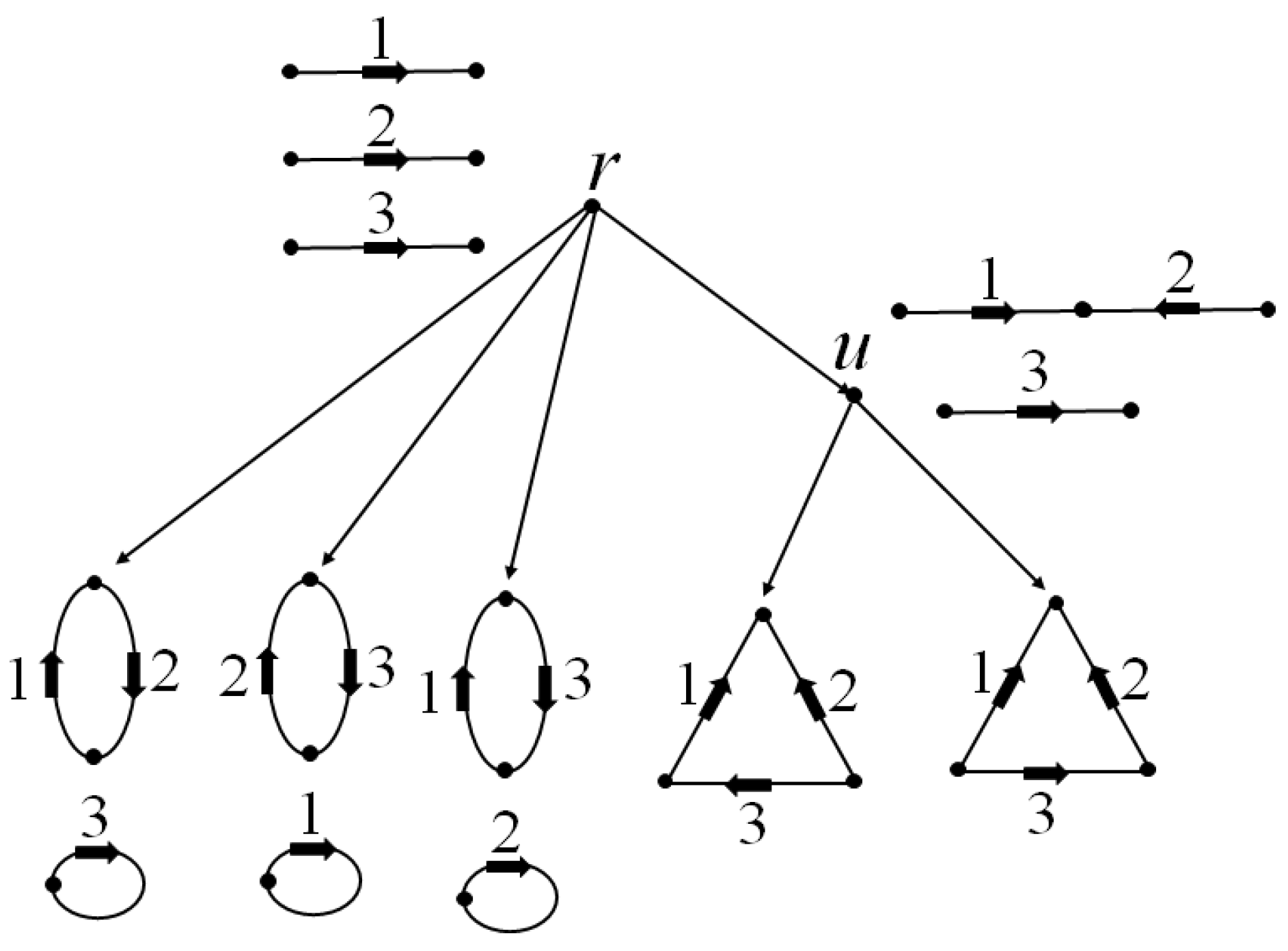
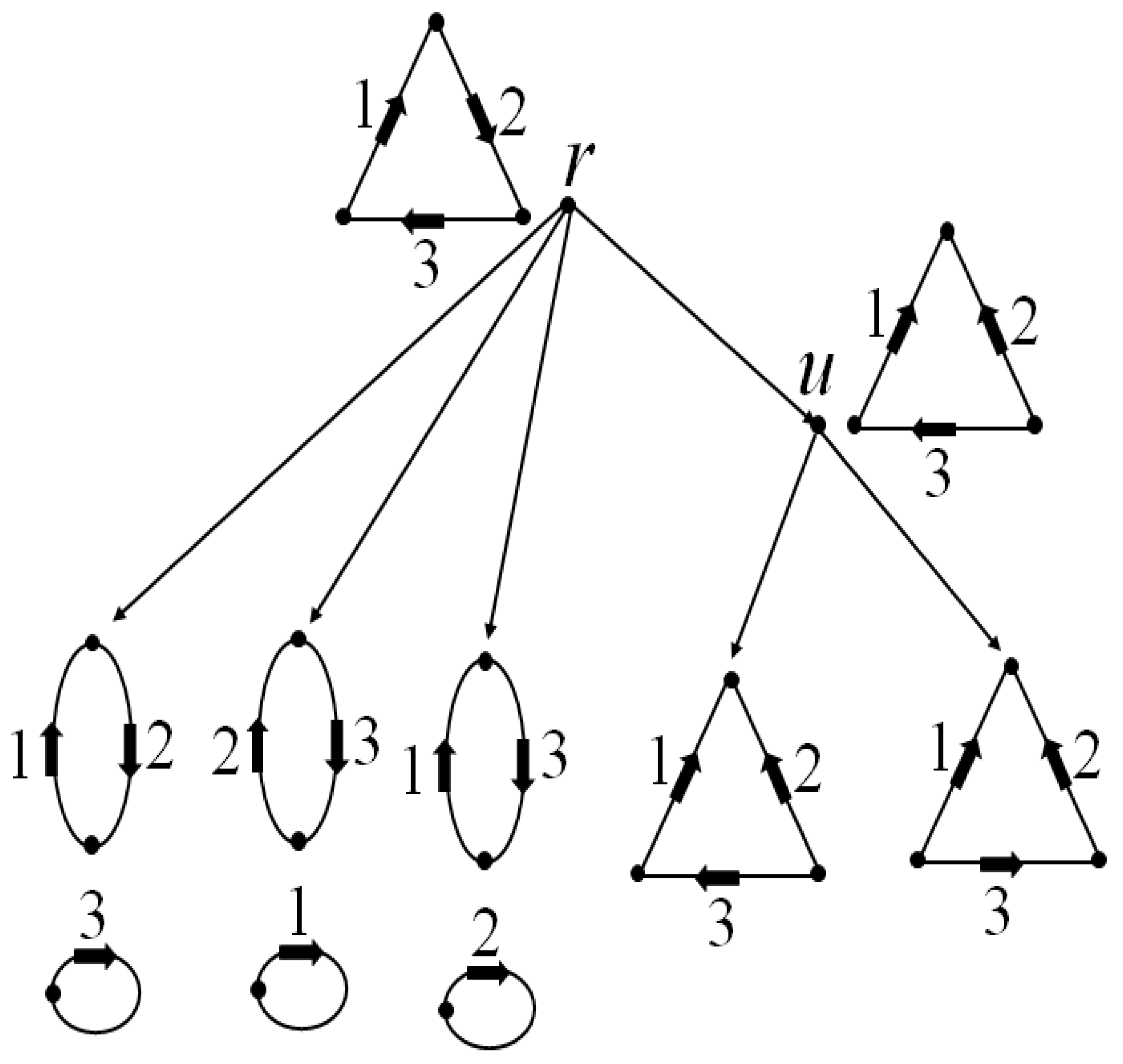
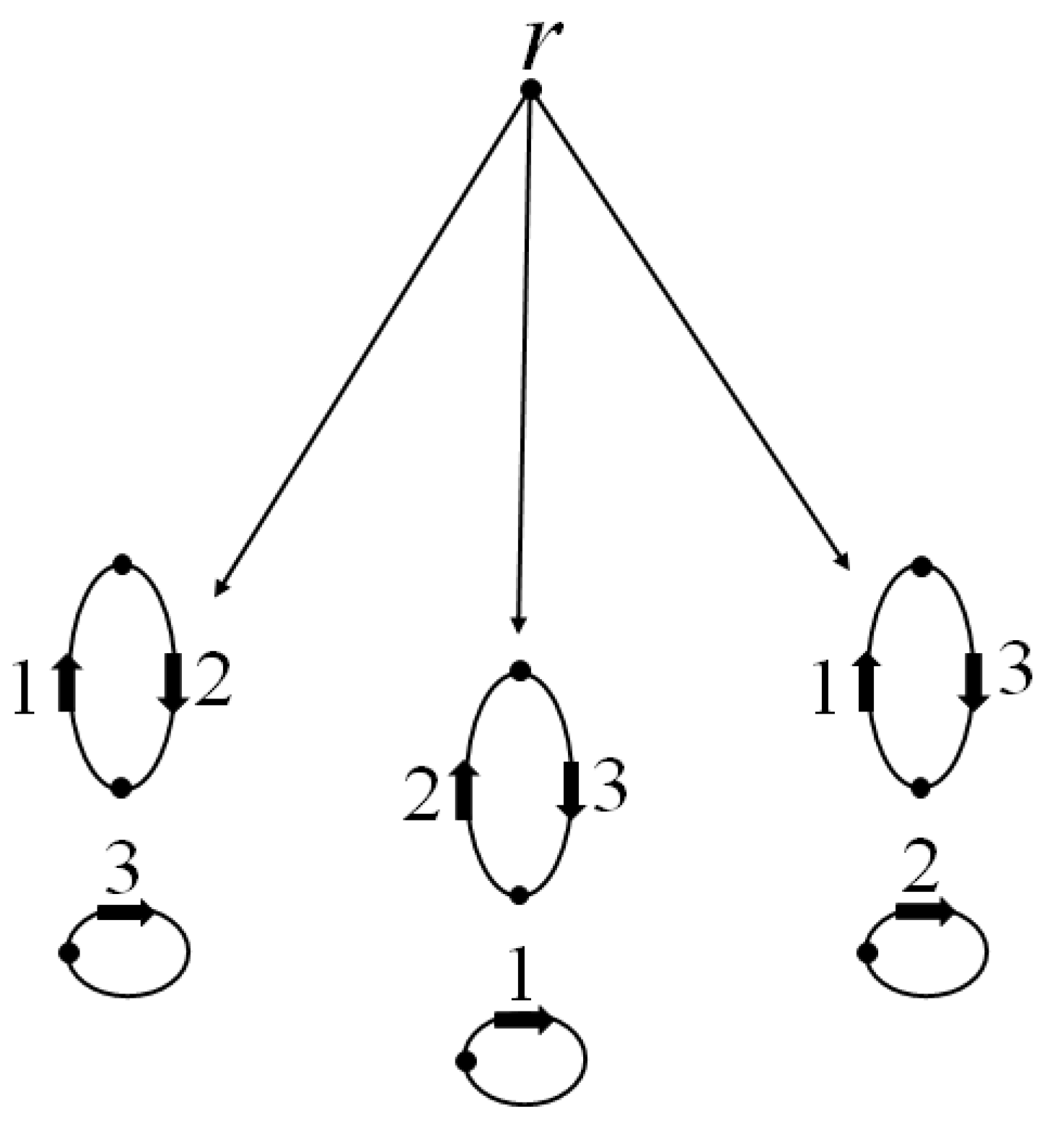
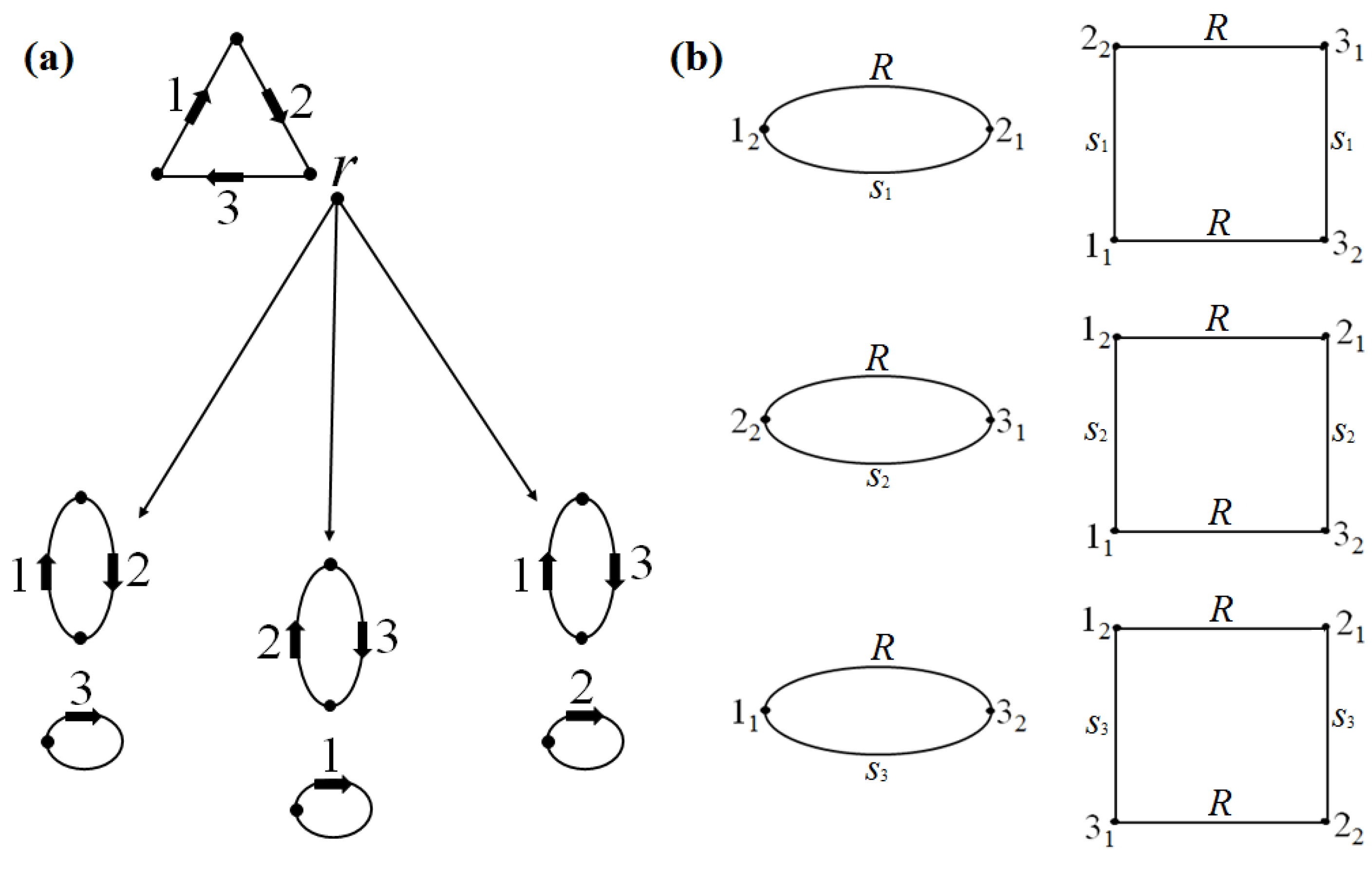
A structure is a directed graph consisting of paths (excluding isolated nodes) and cycles, including loops. Its edges are assigned with unique names; one may assume the names to be positive integers. An extremity is a tail or a head of an edge. A join of two nodes consists of identifying them, and a cut is the operation inverse to the join (see Figure 16). Sometimes, instead of join (two nodes) they say merge, identify, or glue.
There are four operations over a structure, which are called SCJ (Single-Cut-or-Join) operations: cut of its node of degree 2, join of two its nodes of degree 1, deletion of an isolated edge, and insertion of an isolated edge. Each operation is assigned a strictly positive rational number called the cost of the operation. The SCJ distance from a structure a to a structure b is the minimum total cost of operations required to transform a into b. It is easily seen that the SCJ distance equals the weighted sum of the number of pairs of extremities joined in a but not in b, joined in b but not in a, the number of edges that are present in a but not in b, and the number of edges that are present in b but not in a. The SCJ distance is a measure of the evolutionary distance between two structures and is used to construct evolutionary trees and infer evolutionary relationships. The lower the SCJ distance between two structures, the more closely related they are thought to be in terms of their evolutionary history. The same is true for the DCJ distance. The SCJ, as well as the DCJ (Double-Cut-and-Join), operations are well known, and many dozens of papers are devoted to their study, see, e.g., the survey [6] (Section 3).
Additionally, there is another set of operations over a structure, now consisting of six operations, which, in the context of the present paper, will be called DCJ operations, though, usually, this term refers to the first four of them. These are the following operations: cut of a node of degree 2 of the structure, join of two its nodes of degree 1, double and sesquialteral intermerging, deletion, and insertion of a connected fragment of edges. The first two operations are the same as above. The last two are the following, deleting a whole component of a structure (path or cycle) or adding a fragment as a separate component; another option is as follows, such a fragment is cut at its extremities, then it is deleted, and the remaining extremities (if they are two) are joined again; respectively, a node of degree 2 in a structure is cut (or it is a node of degree 1) and the fragment is joined by its extremities (or its extremity) to the obtained extremities (or to the existing extremity). These two operations are generalizations of the corresponding SCJ operations. The third and fourth operations are compositions of the first two. Double intermerging (denoted by DM) consists of cutting a pair of nodes of degree 2 and joining the extremities thus formed with each other. Sesquialteral intermerging (denoted by SM) consists of cutting a node of degree 2 and joining one of the extremities thus formed with a node of degree 1. Quite similarly to the above, each of these operations is assigned with a cost, and the DCJ distance between structures a and b is defined. These operations have long been studied; their detailed description with corresponding figures and historical references can be found in a large number of papers and surveys, e.g., in [6,24,25]. Usually, only four operations are called DCJ operations, Double Intermerging, Sesquialteral Intermerging, and two Ordinary Intermergings (Cut and Join). To a cyclic structure, only the Double Intermerging operation can be applied, because only this operation, being applied to such a structure, preserves its cyclicity and equal content property.
A structure is called cyclic if it consists of cycles only. A set of structures is said to be of equal content of names if all structures in it have the same set of names.
For any tree, an arrangement over it is an assignment of a structure to each interior node of the tree. Arrangements are considered to be specified at leaves; therefore, after specifying them at interior nodes, an arrangement will be set throughout the tree.
The problem of reconstruction is to find structures at interior nodes of the tree so that the resulting arrangement is a minimum of a given functional defined on all arrangements over the given tree. Here, as such a functional, we consider the sum of lengths of all edges of a tree, where the length of an edge is the distance between the structures at its endpoints. As a distance, we consider the SCJ or DCJ distance; where each edge is directed from the root to the leaves of the tree. The value of this functional is called the cost of the arrangement. An arrangement with the lowest cost is said to be minimum, and its cost is referred to as the minimum cost, which is also sometimes called the global minimum. An arrangement is said to be locally minimum if replacing a structure at any interior node of the tree with any other does not reduce the cost of the arrangement.
A star-like tree (or simply a star) is a tree consisting of a root and leaves to which the root is connected. A two-star tree is a tree with two interior nodes (denote them by r and u), such that the root r is connected with arbitrarily many leaves and u is connected with only two leaves (see Figure 17).
Setting of the SCJ and DCJ reconstruction problems. Given: a rooted tree, not necessarily binary, to each leaf of which there is assigned a loopless structure; and arbitrary strictly positive costs of all SCJ or all DCJ operations. Find: an arrangement (at interior nodes of the tree) such that the sum over all edges of the tree of SCJ or DCJ distances between structures at the endpoints of an edge is minimum. These essentially different reconstruction problems are referred to as, respectively, SCJ or DCJ reconstructions.
We distinguish a cyclic reconstruction problem, where all structures specified at the leaves are cyclic, and only cyclic structures can be attributed to internal nodes (i.e., only cyclic arrangements are considered). Such reconstruction problems will be called cyclic. In a cyclic DCJ reconstruction, the SM, join, and cut operations cannot be applied, and, accordingly, in the set of DCJ operations there remain the DM operation and insertion/deletion of a component of a structure.
Another particular case of the reconstruction problem is as follows; structures at the leaves are of equal content, and only arrangements with the same set of names as for the structures at the leaves are considered. In this case, we speak about the equal-content reconstruction problem. In the cyclic equal-content DCJ reconstruction, in addition, the insertion/deletion operations cannot be applied, and accordingly, in the set of DCJ operations there remains the DM operation only. In this case, the cost of this operation can be omitted without loss of generality.
In the reconstruction problems, we prove the following theorems, where n is the number of names in the structures assigned to the leaves and l is the number of leaves.
Theorem 4.
An exact algorithm is constructed which solves the SCJ reconstruction problem on any two-star tree for arbitrary costs of SCJ operations. The runtime of the algorithm is of the order of n2·(l + log(n)).
Recall that the SAT problem for a given conjunctive normal form (CNF) is the problem of determining whether there exist values 0 and 1 of the variables in this CNF for which the CNF equals 1, and if they do exist, giving an example of those values.
Theorem 5.
An exact algorithm is constructed which reduces the cyclic equal-content DCJ reconstruction problem on any star to a sequence of length log(n·l) of SAT problems in which every CNF contains of the order of n2·l2 variables and of the order of n3·l2 disjunction terms.
Numerous references concerning this problem can be found, e.g., in [24]. Let us present results directly related to Theorems 4 and 5. In [10], for equal costs of SCJ operations and equal-content structures, there was described an exact quadratic-time algorithm for structure reconstruction on an arbitrary tree, loops at leaves being admissible. In [26], for equal costs of SCJ operations and arbitrary content of structures, there was described an exact quadratic-time algorithm for structure reconstruction on an arbitrary tree (loops being admissible). In [11], for arbitrary costs of SCJ operations and arbitrary content of structures (but with the condition that structures do not contain loops), there was described an exact algorithm for structure reconstruction on a star. Thus, in Theorem 4 we pass from a star to a two-star tree.
In [24], there was considered a generalization of the SCJ reconstruction problem where each pair of extremities is assigned with a weight, and when this pair is joined, its weight is added to the objective function. Additionally, it was proved there that this problem is NP-hard, and an FTP-algorithm for solving it was described. Namely, there was an algorithm described with a runtime being exponential in one variable only; this variable reflects the number of conflicts at interior nodes of the tree when reconstructing by each pair of extremities separately (for exact formulations; see [24]). The algorithm is based on reduction to an integer linear programming (ILP) problem.
In Theorem 5, the cyclic equal-content DCJ reconstruction problem on a star is reduced to a sequence of SAT problems. Note that the reduction to a SAT solver instead of reduction to an ILP-packet is much more efficient (see [27]).

3.2. SCJ Reconstruction Algorithm

Recall that we consider structures with no loops at the leaves. We will identify a node of a tree and a structure assigned to it. Additionally, we consider only edges contained in at least one leaf structure, such edges will be called admissible. Both constraints do not lose the generality of solution.
If an edge of a leaf structure is not present at some leaf (which is also a structure), we add it there as a loop; then the SCJ reconstruction problem reduces to the case of equal-content structures at leaves and at all interior nodes. Let the cost of joining an isolated edge into a loop be equal to the cost of edge deletion, and the cost of cutting a loop be equal to the cost of adding an isolated edge. Thus, there remain two operations only; join and cut of extremities of an admissible edge, but four costs for them are defined.
Denote the names of the extremities of the ith edge by i1 (tail) and i2 (head). There arises a one-to-one correspondence between structures and matchings on the set (later: a graph) M of names of extremities of all admissible edges. Namely, structure a corresponds to a matching P on M such that the extremities ik and jl are connected by an edge in P if, and only if, ik and jl are joined in a.
Let us be given a two-star tree (Figure 17). Recall that an edge of a tree is considered together with the direction from the root to the leaves. An event for an unordered pair p = (ik,jl), ikjl, on an edge of the tree is passing from being joined at one end of the edge to being cut at another end of it, or vice versa. A p-scenario is a specification of being joined/cut for a fixed pair p at all interior nodes of the tree; at the leaves, this specification is already given. The cost of a p-scenario is the total cost of events with the pair p according to this specification. Note that the set 𝒮 of p-scenarios formed for all pairs p does not necessarily define an arrangement (at interior nodes) on the tree; even if 𝒮 defines an arrangement at the tail i1 of an edge, it need not define a structure in i2, since at i2 one extremity can be joined with two other extremities. Our efforts are aimed to rule out such a situation.
Let us describe the SCJ reconstruction algorithm. We say that an unordered pair p is admissible if its extremities are joined in at least one leaf of the tree. For each admissible pair p, independently of other pairs of edge extremities, we inductively compute (forward pass of the proposed algorithm from the leaves to the root) two quantities, pyes and pno. In each leaf v we set pyes(v) = 0 if p is joined, and pyes(v) = ∞ if it is not joined. Similarly, pno(v) = 0 if p is not joined, and ∞ if it is joined.
In the induction step, we compute:
pyes(v), the minimum cost of all p-scenarios starting at v provided that the pair p is joined at v, and
pno(v), a similar quantity provided that p is not joined at v.
For that, during the forward pass of the algorithm, for every next node v of the tree we consider all its child nodes. For each child v1 of v, we know p1yes and p1no; we compute pyes = min(p1yes, p1no + c1), where c1 is the cost of the corresponding cut, and take the sum over all children. For instance, at node r (see Figure 17), we have p y e s ( r ) = v i min ( p y e s ( v i ) , p n o ( v i ) + c 1 ) , where vi runs over all children of r. If the minimum is attained on the first argument, we record the pointer pyesyes, and otherwise, pyesno, where the first pointer means “join” of the extremities in p at v1, and the second, “no join” of these extremities. Similarly, we compute pno = min(p1yes + c2, p1no), where c2 is the cost of the corresponding join, and take the sum over all children. For instance, at node r (the same figures), we have p n o ( r ) = v i min ( p y e s ( v i ) + c 2 , p n o ( v i ) ) , where vi runs over all children of r. If the minimum is attained at the first argument, we record the pointer pnoyes, and otherwise pnono. Thus, a pair p at v is labeled by pyes, pno, and two pointers, one of them beginning with pyes and the other with pno. These pointers are used in the backward pass of the algorithm when passing from v to v1.
We consider the set M of all extremities at one leaf of the tree (or, equivalently, at all leaves of the tree) as a loopless graph with all admissible unordered edges p. If the edges of the graph M are assigned with weights, which are rational or even integer numbers, then we denote by w(x) the weight of any matching x on M; here, every x is a subgraph in M with nodes of degrees 0 or 1. In other words, a matching is a subset of edges in a given graph where no two edges share a common vertex. To each edge p in M, we can assign the weight pyespno and construct a minimum weighted matching P, which is obtained by minimizing w(x) over all matchings x in M. Thus, at the root r, the structure Pr is defined to be the minimum matching with weights pyespno obtained at the root node r of the tree as a result of the forward pass of the algorithm.
Using the minimum matching Pr, for each edge p in M, by backward pass of the algorithm we uniquely determine whether the pair p is joined at u. Namely, if pPr, then we use the pointer that begins with pyes; if pPr, we use the pointer that begins with pno. Namely, for pyesyes the pair p will be joined at u, and for pyesno it will not be joined at u. However, unlike the Pr, it is not clear whether in this way there will be defined a structure at u. In Lemma 1, it is shown that any extremity at u is joined with at most one extremity; thus, the structure Pr at r defines some structure Pu at u. Therefore, there arises an arrangement {Pr,Pu} on the tree, which is said to be final; this is the output of the algorithm. Of course, this backward pass can be defined for any tree, but in this case Lemma 1 need not necessarily hold. The flow chart of the algorithm is shown in Figure 18.
Denote by s(P) the set 𝒮 of p-scenarios for all unordered admissible pairs p, according to which a pair p is joined at r if, and only if, pP, and a pair p is joined or not joined at u according to the above-mentioned backward pass. Here, we used P at r instead of Pr. Denote by c(P) the total (over all such p) cost of p-scenarios in s(P).

3.3. Exactness and Runtime of the SCJ Reconstruction Algorithm

Denote by P0 the empty matching.
Lemma 1.
For any structure P at the root node r we have c(P) = c(P0) + w(P). The minimum of c(P) is attained at Pr which defines the minimum final arrangement on the tree.
Here, final means that the backward pass of the algorithm defines exactly structures, i.e., any extremity at u is joined with at most one extremity. Thus, the algorithm defines a structure at u.
Proof. 
Any minimum arrangement does not have every unordered pair p joined if p is not joined in at least one leaf of the tree. Therefore, when finding the minimum arrangement, it is possible—as we have done—to confine ourselves only with pairs p that are joined in at least one leaf of the tree, i.e., to confine ourselves with admissible pairs p only.
Recall that pP means that an edge p belongs to a matching PM, and pP means that an edge p in M does not belong to P. The definition of pyes and pno at r implies that for any matching P in M we have
c ( P 0 ) = p P 0 p n o = p P p n o + p P p n o ,   c ( P ) = p P p y e s + p P p n o .
Then, c ( P ) c ( P 0 ) = p P ( p y e s p n o ) = w ( P ) . Therefore, the minimum of c(P) is attained at Pr, since Pr is a minimum matching.
To prove the second claim, assume that at u there are two joined pairs p1 and p2 incident to each other. At each of the three neighbors of u, at least one of the pairs p1 and p2 is not joined by the condition. Since there are exactly three neighbors, at least one of the pairs p1 and p2 (say p1) is not joined at least at two neighbors of u. Then, by making p1 not joined at u, one strictly reduces the cost of the p-scenario, which contradicts the minimality of c(Pr). Thus, the backward pass defines an arrangement with cost c(Pr) over a two-star tree. Assume that there is an arrangement with a cost strictly less than this. It defines some matching P at r. We have c(P) < c(Pr), which contradicts the minimality of c(Pr).
Proof of Theorem 4.
The proposed algorithm consists of the three above-described steps: forward pass, constructing a matching Pr, and backward pass, which defines Pu. The exactness of the algorithm follows from Lemma 1.
The runtime of the algorithm is the sum of the computation time for the three above-mentioned steps. Since the number of admissible p is not greater than nl, the runtime of the first and third steps is of the order of nl. A minimum matching is constructed in a time of the order of n′·m + (n′)2·log(n′), where n′ is the number of nodes in the graph M and m is the number of edges in it, ([28] Chapter 11). Since n′ = 2n and mn·l, this time is of the order of n2·(l + log(n)).
Remark 3.
The described algorithm obviously can be generalized to the case when there are several nodes u (see Figure 17), i.e., any child of the root of the tree is a leaf or a node with exactly two children, which are leaves. For this case, the Proof of Theorem 4 can be literally repeated.

3.4. Example of Executing the SCJ Reconstruction Algorithm

A two-star tree and structures at its leaves are shown in Figure 19. Let the cost of all operations be 1.
At node u we have pyes(u) = 0, pno(u) = 2 for p = (12,22); and similarly pyes = 1, pno = 1 for p = (3i,11) and p = (3i,21), where i is arbitrary; pyes = 2, pno = 0 for other p. At node r we have pyes(r) = 3, pno(r) = 1 for p = (12,22); pyes = 3, pno = 2 for p = (32,11) and p = (32,21); pyes = 4, pno = 1 for p = (31,11) and p = (31,21); pyes = 3, pno = 1 for the seven p that are joined at an r-leaf but not at a u-leaf; and pyes = 4, pno = 0 for other p.
Weights of all pairs are positive; therefore, the minimum matching is empty. Hence, there are no joins at r; following the arrows, we obtain a structure at u. The resulting arrangement is shown in Figure 20; its cost is 14.
Now assume that the cost of a cut of any pair is 1, and the cost of a join is 4. At node u we have pyes(u) = 0, pno(u) = 2 for p = (12,22); and similarly pyes = 1, pno = 4 for p = (3i,11) and p = (3i,21), where i is any; pyes = 8, pno = 0 for other p. At node r we have pyes(r) = 3, pno(r) = 4 for p = (12,22); pyes = 3, pno = 8 for p = (32,11) and p = (32,21); pyes = 4, pno = 4 for p = (31,11) and p = (31,21); pyes = 3, pno = 4 for the seven p that are joined at an r-leaf but not at a u-leaf; and pyes = 4, pno = 0 for other p; a non-zero term arises only on the edge (r,u) for the pair (12,22) when computing pno®.
For weights of the edges in M we obtain the following: –1 for p = (12,22); –5 for p = (32,11) and p = (32,21); 0 for p = (31,11) and p = (31,21); –1 for the seven p that are joined at an r-leaf but not at a u-leaf; and 4 for other p. A minimum matching has weight –7 and consists of the pairs (32,11), (12,21), and (22,31). The resulting arrangement is shown in Figure 21, its cost being 49.

3.5. Heuristic Algorithm for the Cyclic Case of the SCJ Reconstruction Problem on an Arbitrary Tree

The authors are unaware of whether an exact polynomial-time SCJ reconstruction algorithm for a structure over a two-star tree in the cyclic case is possible, even without regard to the costs. A heuristic algorithm for this case can easily be obtained by modifying the algorithm described in Section 3.2. Namely, for Pr we take a minimum complete weighted matching. After that, as described in [11], we could descend to a locally minimum arrangement by alternating replacements of complete matchings at u and at r, beginning from u. At a current node v, a matching is replaced with a minimum complete one with respect to the weights pc = pyespno of unordered pairs p (edges in M), where pyes is the total cost of events with the pair p on edges incident to v provided that it is joined at v, and pno is the similar cost provided that p is not joined at v.
Let all costs be uniform in the example presented in Figure 19; a minimum complete matching Pr is shown in Figure 20. One can easily check that the descent to a local minimum can be made in one step; the resulting arrangement is shown in Figure 22, its cost being 20. In this case, the local minimum is also global.

3.6. DCJ Reconstruction Algorithm

In the cyclic equal-content setting (with only the DM operation), the DCJ reconstruction problem becomes NP-hard even for a tree consisting of a root and three leaves [29]. In [12], a much more general problem of DCJ reconstruction has been exactly reduced to an integer linear programming (ILP) problem.
The cyclic equal-content setting DCJ reconstruction problem considered here is exactly reduced to a sequence of SAT problems. The latter way is preferable, since presently there exist programs, called SAT solvers, which in several minutes verify the satisfiability of a formula with tens of thousands of variables and hundreds of thousands of clauses, and if it is satisfiable, output a satisfying assignment of variables; see, e.g., [27] and the Internet site http://fmv.jku.at/lingeling (accessed on 24 February 2023), where references to the corresponding programs and numerous publications can be found. In the cyclic equal-content setting costs of any arrangements are positive integers. By an admissible edge we call any edge in given structures assigned to leaves of a given tree in the DCJ reconstruction problem. One name at the leaves of the tree exactly corresponds to one admissible edge.
To describe the reduction in the cyclic equal-content DCJ reconstruction problem on a star with tree root r to a sequence of SAT problems, we consider an auxiliary problem:
(*) Does there exist an arrangement (in fact, a structure at r) with a cost no greater than a given positive integer k?
We will decide the (*) problem by finding a SATk problem such that any of its affirmative solution describes a structure R at r in the (*) problem, and the thus-obtained arrangement on a star will be a solution to the auxiliary (*) problem.
It is clear that solving this SATk problem is equivalent to solving problem (*). Because of this, the smallest k* for which the corresponding SATk* problem has an affirmative solution is the lowest arrangement cost in the DCJ reconstruction problem; the corresponding arrangement is minimum. Below a reduction in the (*) problem to a SATk problem is described for every k.
Being able to solve the (*) problem for various k, we can trivially solve the original DCJ reconstruction problem. Let k1 and k2 be such that k1k* ≤ k2. For example, we may set k1 = 0 (in Section 3.8 we present a way to obtain a nontrivial lower estimate for k*) and k2 = nl, where n is the number of names in leaves and l is the number of leaves in a given tree. Given these bounds, k1 and k2, for k we take the integral part [(k1 + k2)/2], and then solve the SATk problem. If the solution is affirmative, we pass to the left-hand part of the segment [k1, k2]; otherwise, to the right-hand one. We again denote this next segment by [k1, k2], and so on. In [log2(k2k1)] + 1 steps, we arrive at a segment k1 = k2 and the desired k* = k1.
Now we describe the conjunctive normal form CNFk, form for any given k. However, first, we describe an important general construction. For two structures, a and b, there was defined a graph a + b, called the breakpoint graph. For equal-content structures, a and b, the breakpoint graph can equivalently be defined simpler, as follows. Consider the set M of extremities of all edges in a (or, equivalently, in b), and in the two matchings on M corresponding to the structures a and b. Then, a + b is defined to be the set of edges in M consisting of the edges belonging to one of these matchings. The minimum number of DM operations required to transform one cyclic equal-content structure a into another b is nx, where n is the number of names in a (or, the same thing, in b), and x is the number of cycles in a + b. This can easily be proved directly. Every edge in a + b corresponds to a pair of joined extremities in a or in b, and, at the same time, corresponds to an edge of one of the two matchings in M corresponding to a and b. In the graph a + b, edges are labeled by successively alternating symbols a or b according to whether this edge belongs, as a joined pair, to a or to b. If a and b are cyclic structures, then a + b is a cyclic graph.
Because of this, the cost y of an arrangement along a star is equal to y = nlx, where x is the total number of cycles (over all leaves s) in all breakpoint graphs R + s, where R is a structure at the root r, and s is the given structure at a leaf s, as well as n is the number of names in leaves and l is the number of leaves in the given tree. Therefore, the existence of an arrangement with cost yk, ref. to (*), is equivalent to the existence of a structure R in r with the total number x of cycles satisfying nlkx. Thus, to reduce the auxiliary problem (*) to a SATk problem, we have to construct a conjunctive normal form CNFk which is satisfiable if, and only, if there exists a matching R on M at r, such that nlkx. Now we construct this CNFk that describes such R on M and estimates the total number of cycles in all R + s from below.
For every unordered pair p = (ik,jl), ikjl, of different extremities in M, we introduce a variable, also denoted by p = (ik,jl), such that at r we have the following, p = 1 if p is joined and p = 0 otherwise. A set of these variables describes the subgraph in M; it can be a matching on M and the desired structure R at r. For each leaf s, for each p joined at s, and for each positive integer m, 1 ≤ mnlk, we introduce a variable psm such that psm = 1 if p belongs to the mth cycle in the set of all cycles in all R + s, where to each m there corresponds a least one cycle different from those corresponding to other m1m; and psm = 0 otherwise. In the first case, m will be called the cycle number of the pair p. If psm = 1, the extremities in p are neighboring in the corresponding cycle.
Let us express the fact that each extremity ijM is joined with exactly one extremity, i.e., values of the variables p on which CNFk takes the value 1 define a partition of M into cycles. For instance, in M there are 4 nodes, denoted by 1, 2, 3, and 4, and for node 1 we write
( ( 1 , 2 ) ¬ ( 1 , 3 ) ¬ ( 1 , 4 ) ) ( ( 1 , 3 ) ¬ ( 1 , 2 ) ¬ ( 1 , 4 ) ) ( ( 1 , 4 ) ¬ ( 1 , 2 ) ¬ ( 1 , 3 ) ) .
In general, we obtain a part of a CNF of the form ∨i ((1,i) ∧ ∧i ¬(1,i′)), where i runs over all nodes in M except for 1, and i′ runs over all nodes in M except for 1 and i. We conjunctively combine these formulae for all other nodes in M except for 1.
The next three parts of CNFk depend on the parameter k. We express the fact that at every leaf s, every joined pair p is assigned with a unique number m. For instance, at leaf s, node 1 is joined with 2 and nlk = 3; i.e., 1 ≤ m ≤ 3. Then, we write a part of the CNF:
( ( 1 , 2 ) s 1 ¬ ( 1 , 2 ) s 2 ¬ ( 1 , 2 ) s 3 ) ( ( 1 , 2 ) s 2 ¬ ( 1 , 2 ) s 1 ¬ ( 1 , 2 ) s 3 ) ( ( 1 , 2 ) s 3 ¬ ( 1 , 2 ) s 1 ¬ ( 1 , 2 ) s 2 ) .
In general, we have ∨m ((i,j)sm ∧ ∧m ¬(i,j)sm), where i and j are joined extremities in s, m running over all cycle numbers and m′ running over all numbers except m. By conjunctively combining such formulae for all other joined p = (i,j) and all leaves s, we obtain ∧psm (i,j)sm ∧ ∧m ¬(i,j)sm. Here, and in what follows, we use structures defined at the leaves. Note that some other qs in the same leaf s (or even in another leaf; see below) may be given the same number m.
Now we express the fact that for every cycle number m (1 ≤ mnlk), at some leaf there exists a joined pair p having this number. For example, there are two leaves; the pairs p joined at leaf 1 are (1,2) and (3,4), and those joined at leaf 2 are (1,3) and (2,4). Then, for every cycle number m we write
( 1 , 2 ) 1 m ( 3 , 4 ) 1 m ( 1 , 3 ) 2 m ( 2 , 4 ) 2 m .
In general, this will be the disjunction of the variables psm over all joined p and all s, for each m separately, p s p s m . By conjunctively combining such formulae for all cycle numbers m, we obtain m p s p s m .
Now let us ensure equality of cycle numbers of all pairs p in each cycle in R + s, for any given leaf s. It suffices to ensure the equality of numbers for neighboring pairs, i.e., for those separated by some joined pair x in R. In other words, we have to ensure the implication that if two joined pair p and q at one leaf s are connected by a joined pair from R, then p and q have the same cycle number m. This is written separately for every cycle number m. For instance, for any joined pairs p = (1,2) and q = (3,4) at the same leaf s, we write (in the parentheses, there are all possible joined pairs in R)
( ( 1 , 3 ) ( 1 , 4 ) ( 2 , 3 ) ( 2 , 4 ) ) ( p s m q s m ) .
Here, psm can be equal to 0; recall that a joined pair xR is an edge in R + s. By conjunctively adding such formulae for all cycle numbers m, all leaves s, and joined pairs p = (p1,p2), q = (q1,q2) in s, we obtain
mspq ( ( p 1 , q 1 ) ( p 1 , q 2 ) ( p 2 , q 1 ) ( p 2 , q 2 ) ) ( p s m q s m ) .
It may seem that we also need to ensure that joined pairs in different cycles have different cycle numbers. However, this is not necessary: if different cycles have the same numbers, the number of cycles will be greater than nlk, which also satisfies the conditions of problem (*). The flow chart of the algorithm is shown in Figure 23.
Proof of Theorem 5.
The description of CNFk expresses the condition nlkx, and the trivial bounds for k* (from 0 to nl) imply the exactness of the reduction. Let us check the estimate for the size of CNFk; in respect of the number of variables, it is obvious. To obtain an estimate for the number of disjunctions, note that Equation (1) is equivalent to a conjunction of four disjunctions:
( ( 1 , 2 ) ( 1 , 3 ) ( 1 , 4 ) ) ( ¬ ( 1 , 2 ) ¬ ( 1 , 3 ) ) ( ¬ ( 1 , 2 ) ¬ ( 1 , 4 ) ) ( ¬ ( 1 , 3 ) ¬ ( 1 , 4 ) ) .
Equation (2) is equivalent to an analogous conjunction. Equation (3) is equivalent to a conjunction of four disjunctions:
( ¬ ( 1 , 3 ) ¬ p s 1 q s 1 ) ( ¬ ( 1 , 3 ) p s 1 ¬ q s 1 )
( ¬ ( 1 , 4 ) ¬ p s 1 q s 1 ) ( ¬ ( 1 , 4 ) p s 1 ¬ q s 1 )
( ¬ ( 2 , 3 ) ¬ p s 1 q s 1 ) ( ¬ ( 2 , 3 ) p s 1 ¬ q s 1 )
( ¬ ( 2 , 4 ) ¬ p s 1 q s 1 ) ( ¬ ( 2 , 4 ) p s 1 ¬ q s 1 ) .
Here, at each leaf there are of the order of n2 pairs (p,q), which in total, over all leaves, gives ln2; this is multiplied by the number nl of cycle numbers.

3.7. Example of the DCJ Reconstruction

It is often reasonable to confine ourselves with a reduced version of the problem: a root structure is sought for among the structures in which any joined pair p of extremities occurs at least at one of the leaves. Our simulation (results are not presented here) shows that a root structure appearing in the DCJ reconstruction usually possesses this property. Then, the number of variables and disjunctions in the corresponding CNFk considerably reduces.
Let us perform the DCJ reconstruction with a reduced version for the input data shown in Figure 24.
For the upper and lower bounds for the parameter k, we take the trivial values k1 = 0 and k2 = nl = 9, where n = 3 is the number of names in leaves and l = 3 is the number of leaves. According to the algorithm in Section 3.6, we construct CNF2, which has nlk = 7, and obtain that it has no affirmative solution; therefore, a structure R is not well defined. Then, we construct CNF3, which has nlk = 6, and obtain that it does have an affirmative solution. The satisfying collection of variables is as follows (we present those equal to 1 only): (12,21), (22,31), (32,11); (12,21)l1, (22,11)l2, (31,32)l2, (22,31)m3, (32,21)m4, (11,12)m4, (12,31)r5, (32,11)r6, (21,22)r6, where the indices l, m, and r indicate, respectively, the left, middle, and right leaves. The first three variables determine a corresponding structure R with six cycles (in total) in all graphs R + s. The resulting arrangement is shown in Figure 25a, and these breakpoint graphs R + s, each of them consisting of two cycles, are shown in Figure 25b.

3.8. Lower Bound on the Parameter k in the Conjunctive Normal Form CNFk and Final Form of a Common Graph

One can improve the lower bound on k* by constructing a common graph G of all leaf structures. This is a graph with node set M, and an edge connects two extremities if they are joined in some leaf structure; the edge is labeled with the name of the corresponding leaf. The common graph of structures a and b is their breakpoint graph. Thus, two nodes can be connected by several (up to l) edges, and the degree of any node of the graph is l, since all the structures are cyclic. A common graph G is said to be of a final form if every one of its connected components is two nodes connected by l edges. This graph G is of a final form if, and only if, it is obtained from identical leaf structures. In a common graph G of a final form there are n connected components where n is the number of names in leaves of the tree. A DM operation over G consists of replacing two edges having the same name with other two edges having the same name and the same four extremities.
A DM operation is invertible, and its inverse is also a DM operation. Therefore, the total number of DM operations in transformations of a root structure r to leaf structures s equals the total number of DM operations in transformations of leaf structures to a root one. Additionally, the latter equals the number of DM operations in the shortest transformation (commonly called reduction) of G to a final form. A cycle in G is said to be alternating if each edge in it is labeled by one of two names and these labels alternate. In a graph of a final form there are nl·(l − 1)/2 alternating cycles (all of length 2). Note the following, any alternating cycle in G is contained in precisely one si + sj where si and sj are any two leaves of the tree. Therefore, the number of alternating cycles in an arbitrary G is not greater than in a final one, and a DM can increase this number by at most l–1. Hence, we obtain a lower estimate of n l 2 d l 1 for the SAT bound, where d is the number of alternating cycles in G. This is a lower bound for k*.
An upper bound for k* can be obtained by exhaustively examining the arrangements in which r is a structure coinciding with a structure at some leaf and by computing the minimum cost among all these arrangements.

4. Discussion

We have described an algorithm for constructing an intermediate tree, which, in particular, makes it possible to determine coordinated evolution of proteins with respect to the genes that encode them, and of these genes themselves with respect to the species that contain them. This has also been performed for an important case where the species tree is represented by a network. We have described algorithms for reconstructing the evolution of structures along the tree, which, in particular, allow the reconstruction of genomic structures along a given tree.
Let us outline possible directions for further research. In the problem of constructing an intermediate tree G, we have proposed a way to construct a collection B of clades for which our algorithm outputs the best reconciliation of G with a preassigned tree P and network S. Further research can be aimed at finding other ways to construct collection B. Additionally, of interest is the case where P is a non-binary tree, along with the problem of optimal binarization of P. A binarization method is described and can easily be adapted for our algorithm, but the problem of choosing an optimal binarization still remains. The question of whether it is possible to remove the constraints on costs of the events in the statement of Theorem 3 so that the described algorithm is still exact also remains open.
The questions of an exact efficient algorithm for SCJ reconstruction on an arbitrary tree for arbitrary costs of SCJ operations and of for DCJ reconstruction even on a two-star tree in the cyclic case remain open.

Author Contributions

Conceptualization, V.L. and K.G.; proof, K.G. and V.L.; writing—original draft preparation, K.G.; writing—review and editing, V.L.; supervision, V.L.; project administration, V.L. All authors have read and agreed to the published version of the manuscript.

Funding

This research was partially funded by RFBR grant 20-01-00670.

Data Availability Statement

Not Applicable.

Conflicts of Interest

The authors declare no conflict of interest.

Appendix A. The Procedure to Construct the Main Parameter of the Algorithm

Given collection B′, exhaustively examining sets from B′ in ascending order of their cardinality (in the case of equal cardinalities, in an arbitrary order). For each successive set A, we perform the first feasible step out of the following five (Steps 1–5).
(1)
If there exists a partition of A into two sets A1 and A2 in B′, then procced with the next set A.
(2)
If there exist two sets, A1 and A2, in the current B′ such that the sets A1A and A2A form a partition of A, consider both of the cases A = AiA with i = 1 and i = 2, and so on over all steps until we obtain one-element sets A. At each step, we add to B′ the sets forming the partition of A; the same in all the following steps.
(3)
If there exists a set A1 in the current B′ such that A1A (take A1 for which |A1| is the largest), consider both of the sets A = A1 and A = A\A1, and so on over all steps until one-element sets for A are obtained.
(4)
If there exists a set A1 in the current B′, such that A1A and A\(A1A) is a partition (take A1 for which |A1A| is the largest), then consider both sets, and so on over all steps until one-element sets are obtained.
(5)
Take any partition of A into two sets A1 and A2 of the same cardinality (with accuracy to 1) and so on over all steps until one-element sets are obtained.
Let us estimate the procedure time for the main parameter B. We consider at most |B′| sets A from the original B′, and for each of them we construct a binary tree with at most |M| nodes. At each node, we consider five cases; the time required to check the conditions of the cases is of the order of at most (|B′|·|M|)2·|M|. Thus, the total time required to construct the collection B is of the order of |B′|3·|M|4. Additionally, a fast version of constructing collection B is possible where, in the conditions of Steps 1–4, we use not the current B′ but rather the original B′. Then, the runtime of the procedure is of the order of |B′|3·|M|2.

References

  1. Li, T.; Yang, B.; Liu, H.; Ju, J.; Tang, J.; Subramanian, S.; Zhang, Z. GMDL: Toward precise head pose estimation via Gaussian mixed distribution learning for students’ attention understanding. Infrared Phys. Technol. 2022, 122, 104099. [Google Scholar] [CrossRef]
  2. Liu, H.; Fang, S.; Zhang, Z.; Li, D.; Lin, K.; Wang, J. MFDNet: Collaborative Poses Perception and Matrix Fisher Distribution for Head Pose Estimation. IEEE Trans. Multimed. 2021, 24, 2449–2460. [Google Scholar] [CrossRef]
  3. Quinlan, J.R. Induction of decision trees. Mach. Learn. 1986, 1, 81–106. [Google Scholar] [CrossRef]
  4. Witten, I.H.; Frank, E. Data Mining: Practical Machine Learning Tools and Techniques with Java Implementations; Morgan Kaufmann: San Francisco, CA, USA. Available online: http://www.cs.waikato.ac.nz/~ml/weka/book.html (accessed on 24 February 2023).
  5. Moayedi, H.; Bui, D.T.; Kalantar, B.; Foong, L.K. Machine-Learning-Based Classification Approaches toward Recognizing Slope Stability Failure. Appl. Sci. 2019, 9, 4638. [Google Scholar] [CrossRef]
  6. Bulteau, L.; Weller, M. Parameterized Algorithms in Bioinformatics: An Overview. Algorithms 2019, 12, 256. [Google Scholar] [CrossRef]
  7. Huson, D.H.; Rupp, R.; Scornavacca, C. Phylogenetic Networks—Concepts, Algorithms and Applications; Cambridge University Press: Cambridge, UK, 2010. [Google Scholar]
  8. Kuitche, E.; Lafond, M.; Ouangraoua, A. Reconstructing protein and gene phylogenies using reconciliation and soft-clustering. J. Bioinform. Comput. Biol. 2017, 15, 1740007. [Google Scholar] [CrossRef]
  9. LeMay, M.; Libeskind-Hadas, R.; Wu, Y.-C. A Polynomial-Time Algorithm for Minimizing the Deep Coalescence Cost for Level-1 Species Nets. IEEE/ACM Trans. Comput. Biol. Bioinform. 2022, 19, 2642–2653. [Google Scholar] [CrossRef]
  10. Feijao, P.; Meidanis, J. SCJ: A Breakpoint-Like Distance that Simplifies Several Rearrangement Problems. IEEE/ACM Trans. Comput. Biol. Bioinform. 2011, 8, 1318–1429. [Google Scholar] [CrossRef]
  11. Gorbunov, K.Y.; Lyubetsky, V.A. Multiplicatively exact algorithms for transformation and reconstruction of directed path-cycle graphs with repeated edges. Mathematics 2021, 9, 2576. [Google Scholar] [CrossRef]
  12. Lyubetsky, V.A.; Gershgorin, R.A.; Gorbunov, K.Y. Chromosome structures: Reduction of certain problems with unequal gene content and gene paralogs to integer linear programming. BMC Bioinform. 2017, 18, 537. [Google Scholar] [CrossRef]
  13. Page, R.D.M. Maps between trees and cladistic analysis of historical associations among genes, organisms and areas. Syst. Biol. 1994, 43, 58–77. [Google Scholar]
  14. Guigo, R.; Muchnik, I.; Smith, T. Reconstruction of ancient molecular phylogeny. Mol. Phylogenet. Evol. 1996, 6, 189–213. [Google Scholar] [CrossRef]
  15. Li, D.; Liu, H.; Zhang, Z.; Lin, K.; Xiong, N. CARM: Confidence-aware recommender model via review representation learning and historical rating behavior. Neurocomputing 2021, 455, 283–296. [Google Scholar] [CrossRef]
  16. Liu, H.; Nie, H.; Zhang, Z.; Li, Y.-F. Anisotropic angle distribution learning for head pose estimation. Neurocomputing 2020, 433, 310–322. [Google Scholar] [CrossRef]
  17. Liu, T.; Liu, H.; Li, Y.-F.; Zengzhao, C.; Zhang, Z.; Liu, S. Flexible FTIR Spectral Imaging Enhancement for Industrial Robot Infrared Vision Sensing. IEEE Trans. Ind. Inform. 2019, 16, 544–554. [Google Scholar] [CrossRef]
  18. Liu, H.; Zheng, C.; Li, D.; Shen, X.; Lin, K.; Wang, J.; Zhang, Z.; Zhang, Z.; Xiong, N. EDMF: Efficient Deep Matrix Factorization with Review Feature Learning for Industrial Recommender System. IEEE Trans. Ind. Inform. 2021, 18, 4361–4371. [Google Scholar] [CrossRef]
  19. Van Iersel, L.; Jones, M.; Weller, M. Embedding Phylogenetic Trees in Networks of Low Treewidth. In Proceedings of the 30th Annual European Symposium on Algorithms (ESA 2022), Berlin/Potsdam, Germany, 5–9 September 2022; pp. 69:1–69:14. [Google Scholar]
  20. Zhang, L. On a Mirkin-Muchnik-Smith conjecture for comparing molecular phylogenies. J. Comput. Biol. 1997, 4, 177–187. [Google Scholar] [CrossRef] [PubMed]
  21. Ma, B.; Li, L.; Zhang, L. From gene trees to species trees. SIAM J. Comput. 2000, 30, 729–752. [Google Scholar] [CrossRef]
  22. Rusin, L.Y.; Lyubetskaya, E.V.; Gorbunov, K.Y.; Lyubetsky, V.A. Reconciliation of Gene and Species Trees. BioMed Res. Int. 2014, 2014, 642089. [Google Scholar] [CrossRef]
  23. Van Iersel, L.; Janssen, R.; Jones, M.; Murakami, Y.; Zeh, N. Polynomial-Time Algorithms for Phylogenetic Inference Problems Involving Duplication and Reticulation. IEEE/ACM Trans. Comput. Biol. Bioinform. 2020, 17, 14–26. [Google Scholar] [CrossRef]
  24. Luhmann, N.; Lafond, M.; Thevenin, A.; Ouangraoua, A.; Wittler, R.; Chauve, C. The SCJ Small Parsimony Problem for Weighted Gene Adjacencies. IEEE/ACM Trans. Comput. Biol. Bioinform. 2019, 16, 1364–1373. [Google Scholar] [CrossRef] [PubMed]
  25. Gorbunov, K.Y.; Lyubetsky, V.A. Linear time additively exact algorithm for transformation of chain-cycle graphs for arbitrary costs of deletions and insertions. Mathematics 2020, 8, 2001. [Google Scholar] [CrossRef]
  26. Gorbunov, K.Y.; Gershgorin, R.A.; Lyubetsky, V.A. Rearrangement and inference of chromosome structures. Mol. Biol. 2015, 49, 327–338. [Google Scholar] [CrossRef]
  27. Sohanghpurwala, A.A.; Hassan, M.W.; Athanas, P. Hardware accelerated SAT solvers—A survey. J. Parallel Distrib. Comput. 2017, 106, 170–184. [Google Scholar] [CrossRef]
  28. Korte, B.; Vigen, J. Combinatorial Optimization. Theory and Algorithms, 6th ed.; Springer: Bonn, Germany, 2018. [Google Scholar]
  29. Tannier, E.; Zheng, C.; Sankoff, D. Multichromosomal median and halving problems under different genomic distances. BMC Bioinform. 2009, 10, 120. [Google Scholar] [CrossRef] [PubMed]
Figure 1. (a) All the considered trees are arranged “top to bottom”; in them, s is a super-root, r a root, and (s,r) a root edge. (b) The mapping s; T1T2 is arbitrarily defined on leaves as a correspondence of labels in which indices are disregarded (i.e., f1 and f2 are mapped to f). The mapping s canonically continues onto interior nodes in T1 as s′: T1T2. For instance, s′(vi) = ui for 1 ≤ i ≤ 4 or i = 6, s′(v5) = u7, and s′(v7) = s′(r) = s′(s) = t. The nodes v7, r, and s are mapped to the root edge. Images of nodes of T1 are shown “inside” T2, so that is why we refer to edges in T2 as pipes.
Mathematics 11 02024 g001
Figure 2. (a) Original tree T1, and (b) its image tree in T2; its nodes are shown in bold, and its edges are shown as polygonal curves. The images of v1 and v2 are located at the same node u5, and the images of v3 and v4 are in the same pipe t. For example, for the edge e′ = (v4,e), its path in T2 is u5u4u2.
Mathematics 11 02024 g002
Figure 3. Mappings s1 and s2 on leaves and their continuations s1′ and s2′ onto interior nodes. We want to minimize c(s1′) + c(s2′) with respect to the gene tree G and thus find a tree G* on which c(s1′) + c(s2′) attains its minimum value.
Mathematics 11 02024 g003
Figure 4. (a) Tree T1 given in Figure 1a above. (b) Image tree isomorphic to T1; marked in red inside T2 (recall that its nodes are shown in bold and its edges are shown as polygonal curves). Here, two duplications, v7 and r, are in the root pipe. Losses: in the edge (v6,f2) at node u3; in the edge (v7,v1) at u5 and u0; in the edge (v5,v2) at u0; in the edge (v5,v3) at u6; and in the edge (r,v6) at u5. All losses are explicit. Interior nodes in T2 are labeled by symbol u with an index. Note that the nodes r, v3, and v4 in Figure 2b are duplications.
Mathematics 11 02024 g004
Figure 5. (a) Edge e enters pipe t: edge e persists at t+ and either becomes lost in t (bold line) or leaves t (dashed line). (b) Edge e leaves the pipe t: edge e arises at t (bold line) or arises above and persists in one of the child pipes of t, passing through the whole t1 or through its part (dashed line).
Mathematics 11 02024 g005
Figure 6. Example of a network: nodes u3, u4, u6, u7, u9, u10, and r are tree-type; nodes u1, u2, u5, and u8 are hybrid; and a, b, c, and d are leaves. There are four groups of nodes.
Mathematics 11 02024 g006
Figure 7. Example of two different minimum embeddings GS with G = ((a1,a2),(a3,a4)) and a network shown in the figure. (a) The edges e1 and e2 neither enter nor leave t. The edge e11 leaves t1. (b) The edge e1 leaves the pipe t because s′ maps e1+ to t and maps e1− strictly below t, and pe1 passes through t1. Similarly, e2 leaves t through t2.
Mathematics 11 02024 g007
Figure 8. The flow chart of the algorithm for Theorem 1. The cost of a partition of A is computed based on the induction assumption that partitions of A1 and A2 and their costs are known.
Mathematics 11 02024 g008
Figure 9. Embedding s′ of the tree P into the tree S. This embedding is constructed according to the definition of an embedding in Section 2.1.
Mathematics 11 02024 g009
Figure 10. Embeddings PG* → S with the tree G* constructed by our algorithm for the main parameter B specified above. These embeddings are constructed according to the definition of an embedding in Section 2.1. (Left): the tree G* with the tree P embedded in it; (right): the tree S with the tree G* embedded in it.
Mathematics 11 02024 g010
Figure 11. Embeddings PGS with the tree G constructed by the algorithm from [8]. These embeddings are constructed according to the definition of an embedding in Section 2.1. (Left): tree G with tree P embedded in it; (right): tree S with tree G embedded in it.
Mathematics 11 02024 g011
Figure 12. Embeddings PG* → S with tree G* constructed by our algorithm for the other main parameter B. These embeddings are constructed according to the definition of an embedding in Section 2.1. (Left): tree G* with tree P embedded in it; (Right): tree S with tree G* embedded in it.
Mathematics 11 02024 g012
Figure 13. (a) Fragment of a network with a given embedding s′ when there is ILS event at t+. (b) The same fragment with the new embedding s″ when there is a loss at z and a duplication at t.
Mathematics 11 02024 g013
Figure 14. The flow chart of the algorithm for Theorem 3.
Mathematics 11 02024 g014
Figure 15. Tree G and its embedding s′ (shown in red) in the network S constructed by our algorithm. In the pipe u7 there is a duplication. The network S was shown in Figure 6.
Mathematics 11 02024 g015
Figure 16. Join (from left to right) and cut (from right to left) of extremities x and y of edges i and j in a structure. The join of the extremities x and y (as two separate nodes in the structure) consists of identifying them as a node z, and the cut means that a node z in a structure is replaced with separate extremities x and y of edges i and j.
Mathematics 11 02024 g016
Figure 17. Two-star tree. Every edge of the tree is directed from the root to leaves.
Mathematics 11 02024 g017
Figure 18. The flow chart of the algorithm for Theorem 4.
Mathematics 11 02024 g018
Figure 19. Example of executing the SCJ reconstruction algorithm: input data at the leaves (two components in each of the three left-hand leaves); all costs are uniform.
Mathematics 11 02024 g019
Figure 20. Result of executing the SCJ reconstruction algorithm (output arrangement): input data at the leaves are shown in Figure 19; all costs are uniform.
Mathematics 11 02024 g020
Figure 21. Result (output arrangement) of executing the SCJ reconstruction algorithm: input data at the leaves are shown in Figure 19, the cost of the cut is 1, and the cost of a join is 4.
Mathematics 11 02024 g021
Figure 22. Result (output arrangement) of executing the heuristic cyclic SCJ reconstruction algorithm; input data at the leaves are shown in Figure 19; all costs are uniform.
Mathematics 11 02024 g022
Figure 23. The flow chart of the algorithm for Theorem 5.
Mathematics 11 02024 g023
Figure 24. Input data at leaves (two cycles at each leaf) for the DCJ reconstruction with a reduced version: reduction to SAT problems.
Mathematics 11 02024 g024
Figure 25. (a) Resulting arrangement in the DCJ reconstruction for the data given in Figure 20, obtained by a reduction to SAT problems. (b) Three corresponding breakpoint graphs R+s, each of them containing two cycles of lengths 2 and 4.
Mathematics 11 02024 g025
Disclaimer/Publisher’s Note: The statements, opinions and data contained in all publications are solely those of the individual author(s) and contributor(s) and not of MDPI and/or the editor(s). MDPI and/or the editor(s) disclaim responsibility for any injury to people or property resulting from any ideas, methods, instructions or products referred to in the content.