Article

Advancing COVID-19 Understanding: Simulating Omicron Variant Spread Using Fractional-Order Models and Haar Wavelet Collocation

1
Department of Mathematics, Faculty of Science, King Khalid University, Abha 62529, Saudi Arabia
2
Department of Mathematics, Faculty of Science, King Mongkut’s University of Technology Thonburi (KMUTT), 126 Pracha-Uthit Road, Bang Mod Thrung Khru, Bangkok 10140, Thailand
*
Author to whom correspondence should be addressed.
Mathematics 2023, 11(8), 1925; https://doi.org/10.3390/math11081925
Submission received: 22 March 2023 / Revised: 14 April 2023 / Accepted: 15 April 2023 / Published: 19 April 2023

Abstract

:
This study presents a novel approach for simulating the spread of the Omicron variant of the SARS-CoV-2 virus using fractional-order COVID-19 models and the Haar wavelet collocation method. The proposed model considers various factors that affect virus transmission, while the Haar wavelet collocation method provides an efficient and accurate solution for the fractional derivatives used in the model. This study analyzes the impact of the Omicron variant and provides valuable insights into its transmission dynamics, which can inform public health policies and strategies that are aimed at controlling its spread. Additionally, this study’s findings represent a significant step forward in understanding the COVID-19 pandemic and its evolving variants. The results of the simulation showcase the effectiveness of the proposed method and demonstrate its potential to advance the field of COVID-19 research. The COVID epidemic model is reformulated by using fractional derivatives in the Caputo sense. The existence and uniqueness of the proposed model are illustrated in the model, taking into account some results of fixed point theory. The stability analysis for the system is established by incorporating the Hyers–Ulam method. For numerical treatment and simulations, we apply the Haar wavelet collocation method. The parameter estimation for the recorded COVID-19 cases in Pakistan from 23 June 2022 to 23 August 2022 is presented.

1. Introduction

The global pandemic caused by SARS-CoV-2, a spike protein virus, has resulted in widespread infections of coronavirus. The severe acute respiratory syndrome (SARS) epidemic in China in 2003 and the Middle East respiratory syndrome (MERS) epidemic in Saudi Arabia in 2012 [1] were both coronavirus epidemics. Coronaviruses are a large family of viruses. The World Health Organization (WHO) first noted a SARS coronavirus 2 (COVID-19) outbreak in Wuhan, China, in December 2019. In March 2020, the WHO declared the outbreak to be a global pandemic. Over 6.6 million COVID-19 deaths [2] have been reported as of 8 January 2023, with over 659 million confirmed cases worldwide. Despite the fact that the disease is primarily transmitted through respiratory droplets produced by breathing, coughing, sneezing, and talking [3,4,5], more research indicates that it may also be transmitted through the air [6,7,8,9]. Additionally, COVID-19 can be acquired by coming into contact with contaminated objects. The virus can cause symptoms such as coughing, muscle pain, vertigo, high temperature, loss of smell, throat irritation, weakness, and nasal congestion and has an incubation period of 2–14 days.
The COVID-19 Omicron variant, which was first identified in South Africa in November 2021, has since raised serious concerns among public health authorities throughout the world, including in Pakistan. The COVID-19 virus, SARS-CoV-2, is thought to be more contagious and potentially more resistant to current vaccinations than earlier SARS-CoV-2 variants. The possibility of the virus spreading further in communities as a result has raised concerns, especially in regions with high population densities and low vaccination rates. The Omicron variant has been found in Pakistan’s major cities such as Karachi, Lahore, and Islamabad as well as other regions of the nation. In response to the threat posed by the variant, the government has increased testing and contact tracing efforts, increased vaccination efforts, and implemented stricter public health measures such as social seclusion and mask use. Despite these initiatives, the situation is still worrying because COVID-19 cases are still on the rise across much of the nation. This emphasizes the requirement for ongoing watchfulness and a thorough, multifaceted strategy to stop the virus’s spread. Along with public health initiatives, this also entails work intended to improve vaccination rates and access, as well as ongoing studies into the biology and epidemiology of the Omicron variant to better understand its potential effects on society. In the end, it will take a concerted effort from all facets of society, including the government, healthcare professionals, and the general public, to stop the spread of COVID-19 and its variants in Pakistan. By working together, it may be possible to reduce the impact of the Omicron variant and protect the health and well-being of communities in Pakistan.
Modeling the spread of the COVID-19 pandemic has been essential in guiding public health policies and interventions as it has been a significant global health crisis. Multiscale modeling techniques have become an effective method for understanding the intricate dynamics of virus pandemics and have been heavily utilized in the case of COVID-19 [10,11]. Epidemiological models have been extensively used to study the dynamics of COVID-19 transmission at the macroscopic level. These models span a spectrum ranging from straightforward compartmental models, such as the susceptible-infected-recovered (SIR) model, to more intricate models that take into account spatial and temporal heterogeneity, demographic factors, and interventions, such as vaccination and social isolation [12,13]. Additionally, the behavior of individual agents and their interactions during the COVID-19 outbreak have been simulated using agent-based models. Network models have been used to study the dissemination of COVID-19 within social networks and communities at the mesoscopic level. These models take into account the variation in contact patterns as well as the effects of social isolation policies on the dynamics of transmission. Large-scale datasets have also been analyzed to find patterns and trends in the spread of COVID-19 [14,15] using data-driven approaches, such as machine learning and artificial intelligence techniques. Models have been created to study the molecular interactions between the virus and host cells at the microscopic level. These models include the structural modeling of virus proteins and their interactions with host cell receptors (see, for example, [16,17]), as well as molecular dynamics simulations. These methods have been applied to comprehend the molecular mechanisms of virus replication and infection and to find potential therapeutic targets. Along with these conventional modeling techniques, there is growing interest in the use of multiscale models, which combine various modeling scales to capture the intricate relationships between virus spread, individual behavior, and public health policies. These models seek to offer a more thorough understanding of the COVID-19 dynamics and assist in the creation of efficient interventions and policies. Multiscale modeling has generally been shown to be an effective method for analyzing the COVID-19 epidemic and informing public health policies and interventions. Multiscale modeling techniques offer a promising way to deepen our understanding of this intricate global health crisis, even though there is still much to learn about the dynamics of COVID-19.
Fractional order differential equations (FODs) have been used to gain a deeper understanding of diseases, and mathematical models have been formulated and studied for various diseases [18,19,20,21,22,23]. The process of differentiation and integration in fractional calculus is generalized to non-integer orders, making it a valuable tool for research in various fields [24]. Caputo–Fabrizio (CF) operators [25], which use non-singular kernels, are one type of fractional derivative that has been developed to overcome the limitations of the ordinary operator. However, the CF operator has a locality problem, leading to the proposal of Mittag-Leffler kernels as a novel type of fractional derivative by Atangana and Baleanu [26]. Overall, the use of fractional calculus and mathematical models can provide insights into the dynamics of infectious diseases and inform public health policy. Omame et al. [27] explore the potential impact of COVID-19 on the dynamics of dengue and HIV transmission in their paper titled “Assessing the impact of SARS-CoV-2 infection on the dynamics of dengue and HIV via fractional derivatives”. Using fractional calculus, the study creates mathematical models and suggests that the pandemic could significantly affect the transmission and control of these diseases. The authors emphasize the importance of considering multiple infectious diseases during pandemics. In their paper “Backward bifurcation and optimal control in a co-infection model for SARS-CoV-2 and ZIKV” [28], the authors present a mathematical model for the co-infection of SARS-CoV-2 and ZIKV. The study examines the role of backward bifurcation in the dynamics of the co-infection and evaluates the potential benefits of optimal control strategies. The study highlights the importance of considering multiple infectious diseases and optimal control strategies in public health policy.
Furthermore, fractional operators with non-singular and singular kernels have been proposed in several works [29,30,31], and research related to these topics and their applications can be found in a number of recent publications [32,33,34,35,36]. As of late, a number of studies have appeared in mathematical modeling that investigate addressing social issues, such as criminal issues, using FCs. A time lag exists between the individual’s offense and the judgment, which is why Bansal et al. [37] introduced the time-delay coefficient to extend the proposed fractional-order crime transmission model to the delayed model. With regard to analyzing crime congestion, in their study, Pritam et al. [38] examined a mathematical model of crime transmission using a fractional-order derivative that includes memory effects, allowing for the previous input’s impact to be taken into account when forecasting the growth rate of crime. Using the iterative fractional-order Adams–Bashforth approach, ref. [39] found the approximate solution and numerically simulated it for various control strategies in different fractional orders.
In recent years, there has been a growing interest in the use of Haar wavelet numerical methods for solving problems related to the COVID-19 pandemic. These methods have been used to model the spread of the virus over time, taking into account the various factors that influence its transmission. The results of these studies have provided valuable insights into the dynamics of the pandemic and its evolution and have informed public health policies and strategies aimed at controlling its impact. Overall, Haar wavelet numerical methods have proven to be a valuable tool for solving problems with fractional derivatives and have been widely adopted in various fields due to their efficiency and accuracy. With ongoing research and development, they are expected to play an increasingly important role in solving complex problems in the future.
Similarly, wavelet analyses have been extensively applied in numerical analyses, statistical applications, image digital processing, quantum field theory, and many other fields. A wide range of applications has been made for Haar wavelets, including in communication and physics research as well as more mathematically-based research on differential equations and nonlinear problems [40]. There is an emphasis on Haar wavelets among all wavelet families. In mathematics, they are the simplest wavelet family because they consist of pairs of piecewise constant functions. In addition, Haar wavelets can also be integrated analytically in random times. Recently, researchers applied this technique for solving different fractional-order mathematical models [41,42]. In addition to being a fast method, the method is also more stable.

2. Preliminaries

The definition of the fractional derivative has developed greatly in recent years [43,44], ranging from the non-singular kernel derivatives and Riemann–Liouville (RL) fractional derivative without a singular kernel to the two-parameter derivative with non-singular and non-local kernels [45]. The two most commonly used definitions are described below:
Definition 1.
The fractional derivative of y of order δ is defined by Riemann–Liouville as follows [42]:
D * δ F ( t ) = 1 Γ ( s δ ) d d t s 0 t F ( ν ) ( t ν ) δ s + 1 d ν , 0 s 1 < δ < s , s N , ( d / d t ) s F ( t ) , δ = s , s N .
Definition 2.
The Caputo fractional derivative of the function F of order δ is defined as follows [42]:
D * δ F ( t ) = 1 Γ ( s δ ) 0 t ( d / d ν ) s F ( ν ) ( t ν ) δ s + 1 d ν , 0 s 1 < δ < s , s N , ( d / d t ) s F ( t ) , δ = s , s N .
Also used in this study is the RL form of the fractional integral operator D * δ of order δ , which is defined as follows:
D * δ F ( t ) = 1 Γ ( δ ) 0 t F ( ν ) ( t ν ) δ 1 d ν

Haar Wavelets

If ψ ( t ) and ψ ˜ 0 ( t ) represent the mother Haar wavelet function (on the real line) and Haar scaling function, respectively, then they are given by [46,47]:
ψ ( t ) = 1 , if t 0 , 1 2 , 1 , if t 1 2 , 1 , 0 , elsewhere ,
ψ ˜ 0 ( t ) = 1 , if t [ 0 , 1 ) .
As a result, if the various Haar wavelets that are produced on the interval [ 0 , 1 ) using multiresolution analysis are ψ ˜ m ( t ) , then:
ψ ˜ m ( t ) = 2 j / 2 ψ 2 j t p , m = 1 , 2 , ;
where m = 2 j + p : p = 0 , 1 , , 2 j 1 ; j = 0 , 1 , . Furthermore, we can translate the Haar functions on u 1 t < u as
ψ ˜ u , m ( t ) = ψ ˜ m ( t + 1 u ) , m = 0 , 1 , 2 , , u = 1 , 2 , , ϱ , ϱ N .
The resulting sequence ψ ˜ m ( t ) m = 0 forms a complete orthonormal system [47] in L 2 [ 0 , 1 ) . Similarly, the sequence ψ ˜ u , m ( t ) m = 0 , u = 1 , 2 , , ϱ , forms a complete orthonormal system in L 2 [ 0 , ϱ ) . Therefore, any function F ( t ) L 2 [ 0 , ϱ ) can be expanded in terms of Haar orthonormal basis functions as
F ( t ) = u = 1 ϱ m = 0 G u , m ψ ˜ u , m ( t ) .
Additionally, after truncating the series F ( t ) , we obtain the equivalent approximation y p ( t ) of F ( t ) as
F ( t ) y p ( t ) = u = 1 ϱ m = 0 p 1 G u , m ψ ˜ u , m ( t ) = B ϱ p × 1 T ψ ˜ ϱ p × 1 ( t ) ,
where the coefficients G u , m can be expressed by the inner product
F ( t ) , ψ ˜ u , m ( t ) = u 1 u F ( t ) ψ ˜ u , m ( t ) d t , m = 1 , 2 , , ( p 1 ) , u = 1 , 2 , , ϱ , B ϱ p × 1 = G 1 , 0 , , G 1 , p 1 , G 2 , 0 , , G 2 , p 1 , , G ϱ , 0 , , G ϱ , p 1 T , ψ ˜ ϱ p × 1 = ψ ˜ 1 , 0 , , ψ ˜ 1 , p 1 , ψ ˜ 2 , 0 , , ψ ˜ 2 , p 1 , , ψ ˜ ϱ , 0 , , ψ ˜ ϱ , p 1 T ,
and superscript T indicates the transpose of a matrix.

3. Mathematical Model

Understanding and forecasting the spread of infectious illnesses are greatly aided by mathematical modeling. Researchers can model how illnesses behave and spread within communities using mathematical equations and algorithms. As a result, they can forecast how the disease will develop in the future and can try different intervention techniques. In addition to helping to identify risk factors and guide public health policy, mathematical models can offer important insights into the fundamental mechanisms of disease transmission. It is crucial to keep in mind that the correctness of these models depends on the caliber of the data input and model assumptions, and they should always be utilized in conjunction with other information sources. Regarding the work of [6,7], the model used consists of the following ODEs:
d S ( t ) d t = B θ S ( t ) I ( t ) ( 1 + τ I ( t ) ) ( ε 1 + ρ + η ) S ( t ) + K V ( t ) , d V ( t ) d t = π S ( t ) ψ V ( t ) ( K + ρ ) V ( t ) , d E ( t ) d t = θ S ( t ) I ( t ) ( 1 + τ I ( t ) ) + ψ V ( t ) ( ε 2 + ρ + φ ) E ( t ) , d I ( t ) d t = φ E ( t ) ( λ + ϵ + ρ + ε 3 ) I ( t ) , d Q ( t ) d t = ε 1 S ( t ) + ε 2 E ( t ) + ε 3 I ( t ) ( ρ + σ ) Q ( t ) , d R ( t ) d t = η S ( t ) + σ Q ( t ) + λ I ( t ) ρ R ( t ) , S ( t ) 0 , V ( t ) 0 , E ( t ) 0 , I ( t ) 0 , Q ( t ) 0 , R ( t ) 0 .
A representation of COVID-19 transmission is provided by the system of ordinary differential equations in mathematical model refe1; the model is divided into six compartments, each representing a different group of people in the population that is affected by the disease. These compartments are as follows: susceptible people S ( t ) , vaccinated people V ( t ) , exposed people E ( t ) , infectious people I ( t ) , quarantined people Q ( t ) , and recovered people R ( t ) . Susceptible people have not been infected but can contract the virus, whereas vaccinated people have received a vaccine and are immune to the virus. Exposed people have been infected but have not yet developed symptoms, whereas infectious people are infected and can spread the virus. Individuals quarantined have been identified as infected and are being isolated to prevent further transmission. Finally, recovered individuals have recovered from the disease and are now immune.
Numerous parameters that affect the dynamics of the disease are included in the model for predicting the spread of COVID-19. The following parameters make up this list: birth rate (B), transmission rate ( θ ), infectivity coefficient ( τ ), quarantine rates for exposed and susceptible individuals ( ε 2 ) and ( ε 1 ) and for natural deaths ( ρ ), vaccination efficacy rate ( η ), vaccination rate ( K ), vaccination loss rate ( ψ ), rate of susceptibility to vaccination ( π ), progression rate ( φ ), recovery rate ( λ ), disease-induced death rate ( ϵ ), quarantine rate for infectious individuals ( ε 3 ), and quarantine loss rate ( σ ). The model’s differential equations predict how these parameters and variables will change over time to affect how many people are in each compartment. It is possible to forecast the spread of COVID-19 and assess the effects of different interventions, such as vaccination and quarantine, by simulating the model.

3.1. Formulation of Fractional Model

The ability to model with fractional-order derivatives, which can more precisely capture the dynamics of some diseases that exhibit non-integer order behavior, is one benefit of using the Caputo derivative over the classical derivative in the context of disease modeling. Because the fractional-order derivatives can capture both memory effects and the power-law decay characteristic of many disease models, this can result in more accurate predictions and better control strategies. The Caputo derivative is also a more economical option for disease modeling because it frequently requires fewer computational resources and data. Additionally, the majority of natural phenomena, including epidemiological dynamics, exhibit the time memory effect. Model (11) is expressed in integral form as:
d S ( t ) d t = t 0 t ς ( t ϖ ) B θ S ( t ) I ( t ) ( 1 + τ I ( t ) ) ( ε 1 + ρ + η ) S ( t ) + K V ( t ) d ϖ , d V ( t ) d t = t 0 t ς ( t ϖ ) π S ( t ) ψ V ( t ) ( K + ρ ) V ( t ) d ϖ , d E ( t ) d t = t 0 t ς ( t ϖ ) θ S ( t ) I ( t ) ( 1 + τ I ( t ) ) + ψ V ( t ) ( ε 2 + ρ + φ ) E ( t ) d ϖ , d I ( t ) d t = t 0 t ς ( t ϖ ) φ E ( t ) ( λ + ϵ + ρ + ε 3 ) I ( t ) d ϖ , d Q ( t ) d t = t 0 t ς ( t ϖ ) ε 1 S ( t ) + ε 2 E ( t ) + ε 3 I ( t ) ( ρ + σ ) Q ( t ) d ϖ , d R ( t ) d t = t 0 t ς ( t ) η S ( t ) + σ Q ( t ) + λ I ( t ) ρ R ( t ) d ϖ .
Incorporating the Caputo derivative, we get
C D t δ 1 d S ( t ) d t = C D t δ 1 I ( δ 1 ) B θ S ( t ) I ( t ) ( 1 + τ I ( t ) ) ( ε 1 + ρ + η ) S ( t ) + K V ( t ) , C D t δ 1 d V ( t ) d t = C D t δ 1 I ( δ 1 ) π S ( t ) ψ V ( t ) ( K + ρ ) V ( t ) , C D t δ 1 d E ( t ) d t = C D t δ 1 I ( δ 1 ) θ S ( t ) I ( t ) ( 1 + τ I ( t ) ) + ψ V ( t ) ( ε 2 + ρ + φ ) E ( t ) , C D t δ 1 d I ( t ) d t = C D t δ 1 I ( δ 1 ) φ E ( t ) ( λ + ϵ + ρ + ε 3 ) I ( t ) , C D t δ 1 d Q ( t ) d t = C D t δ 1 I ( δ 1 ) ε 1 S ( t ) + ε 2 E ( t ) + ε 3 I ( t ) ( ρ + σ ) Q ( t ) , C D t δ 1 d R ( t ) d t = C D t δ 1 I ( δ 1 ) η S ( t ) + σ Q ( t ) + λ I ( t ) ρ R ( t ) .
After calculations, we reach
C D t δ S ( t ) = B θ S ( t ) I ( t ) ( 1 + τ I ( t ) ) ( ε 1 + ρ + η ) S ( t ) + K V ( t ) , C D t δ V ( t ) = π S ( t ) ψ V ( t ) ( K + ρ ) V ( t ) , C D t δ E ( t ) = θ S ( t ) I ( t ) ( 1 + τ I ( t ) ) + ψ V ( t ) ( ε 2 + ρ + φ ) E ( t ) , C D t δ I ( t ) = φ E ( t ) ( λ + ϵ + ρ + ε 3 ) I ( t ) , C D t δ Q ( t ) = ε 1 S ( t ) + ε 2 E ( t ) + ε 3 I ( t ) ( ρ + σ ) Q ( t ) , C D t δ R ( t ) = η S ( t ) + σ Q ( t ) + λ I ( t ) ρ R ( t ) .

3.2. Basic Reproductive Number R 0

The basic reproductive number R 0 , which expresses the typical number of secondary infections caused by a single infected person in a population that is fully susceptible, is an essential component of epidemiological modeling. The advantages of R 0 in epidemiological modeling are extensive: it offers a precise measurement of a disease’s transmissibility, where a disease is more contagious if its R 0 is high, whereas a low R 0 suggests that it is less contagious; predicting the potential spread of an outbreak, which helps epidemiologists forecast the size and length of an outbreak and create the most efficient control strategies by calculating R 0 ; it can be employed to assess the efficacy of interventions, and epidemiologists can assess the success of an intervention in reducing transmission by comparing the R 0 before and after the implementation of a vaccine or quarantine measures; it is useful for locating the crucial control points, and the amount of infected people in a population, for example, is one of the crucial factors in the transmission of an infection that R 0 can be used to pinpoint; and the herd immunity threshold can be predicted using the number, and the percentage of the population that must be immune to a disease for there to be herd immunity is known as the herd immunity threshold. The herd immunity threshold and subsequently the overall efficacy of vaccination programs are predicted with the aid of R 0 . Overall, R 0 is a useful tool for understanding the spread of infectious diseases and for designing effective public health interventions.
The DFE of Model (14) is denoted by E 0 = ( S 0 , V 0 , 0 , 0 , Q 0 , R 0 ) , where
S 0 = B η + ρ + ε 1 , V 0 = π S 0 K + ρ , Q 0 = ε 1 S 0 ρ + τ , R 0 = η S 0 + τ Q 0 ρ .
Our proposed model is split into two matrices [48].
U ˜ = 0 θ S 0 0 0 , V ˜ = φ + ρ + ε 2 0 φ ρ + ϵ + λ + ε 3 ,
V ˜ 1 = 1 ( φ + ρ + ε 2 ) ( ρ + ϵ + λ + ε 3 ) ρ + ϵ + λ + ε 3 0 φ φ + ρ + ε 2 ,
U ˜ V ˜ 1 = θ S 0 φ ( φ + ρ + ε 2 ) ( ρ + ϵ + λ + ε 3 ) θ S 0 ρ + ϵ + λ + ε 3 0 0 .
Hence,
R 0 = φ θ B ( η + ρ + ε 1 ) ( φ + ρ + ε 2 ) ( ρ + ϵ + λ + ε 3 ) .

4. Existence and Uniqueness

The solution for the system (14) using the Caputo operator will be described below, along with its existence and uniqueness. Assume that the continuous real-valued function A ( Y ) , which has the sup-norm property, is a Banach space on J = [ 0 , b ] and that Y = [ 0 , κ ] and P = A ( Y ) × A ( Y ) × A ( Y ) × A ( Y ) × A ( Y ) with norm S , V , E , Q , I , R = S + V + E + Q + I + R , where S = sup t Y | S ( t ) | , V ( t ) = sup t Y | V ( t ) | , E ( t ) = sup t Y | E ( t ) | , Q = sup t Y | Q ( t ) | , I = sup t Y | I ( t ) | , R = sup t Y | R ( t ) | . The following equation is obtain by using the Caputo fractional integral operator on both sides of (14):
S ( t ) S ( 0 ) = C D 0 , t δ S ( t ) B θ S I ( t ) ( 1 + τ I ) ( ε 1 + ρ + η ) S ( t ) + K V ( t ) , V ( t ) V ( 0 ) = C D 0 , t δ V ( t ) π S ( t ) ψ V ( t ) ( K + ρ ) V ( t ) , E ( t ) E ( 0 ) = C D 0 , t δ E ( t ) θ S ( t ) I ( t ) ( 1 + τ I ( t ) ) + ψ V ( t ) ( ε 2 + ρ + φ ) E ( t ) , I ( t ) I ( 0 ) = C D 0 , t δ I ( t ) φ E ( t ) ( λ + ϵ + ρ + ε 3 ) I ( t ) , Q ( t ) Q ( 0 ) = C D 0 , t δ Q ( t ) ε 1 S ( t ) + ε 2 E ( t ) + ε 3 I ( t ) ( ρ + σ ) Q ( t ) , R ( t ) R ( 0 ) = C D 0 , t δ R ( t ) η S ( t ) + σ Q ( t ) + λ I ( t ) ρ R ( t ) .
After calculation,
S ( t ) S ( 0 ) = H ( δ ) 0 t ( t ϖ ) δ B 1 ( δ , ϖ , S ( ϖ ) ) d ϖ , V ( t ) V ( 0 ) = H ( δ ) 0 t ( t ϖ ) δ B 2 ( δ , ϖ , V ( t ) ( ϖ ) ) d ϖ , E ( t ) E ( 0 ) = H ( δ ) 0 t ( t ϖ ) δ B 2 ( δ , ϖ , E ( t ) ( ϖ ) ) d ϖ , I ( t ) I ( 0 ) = H ( δ ) 0 t ( t ϖ ) δ B 4 δ , ϖ , I ( t ) ( ϖ ) d ϖ , Q ( t ) Q ( 0 ) = H ( δ ) 0 t ( t ϖ ) δ B 3 δ , ϖ , Q ( t ) ( ϖ ) d ϖ , R ( t ) R ( 0 ) = H ( δ ) 0 t ( t ϖ ) δ B 5 ( δ , ϖ , R ( t ) ( ϖ ) ) d ϖ ,
where
S ( t ) S ( 0 ) = C D 0 , t δ S ( t ) B θ S ( t ) I ( t ) ( 1 + τ I ( t ) ) ( ε 1 + ρ + η ) S ( t ) + K V ( t ) , V ( t ) V ( 0 ) = C D 0 , t δ V ( t ) π S ( t ) ψ V ( t ) ( K + ρ ) V ( t ) , E ( t ) E ( 0 ) = C D 0 , t δ E ( t ) θ S ( t ) I ( t ) ( 1 + τ I ( t ) ) + ψ V ( t ) ( ε 2 + ρ + φ ) E ( t ) , I ( t ) I ( 0 ) = C D 0 , t δ I ( t ) φ E ( t ) ( λ + ϵ + ρ + ε 3 ) I ( t ) , Q ( t ) Q ( 0 ) = C D 0 , t δ Q ( t ) ε 1 S ( t ) + ε 2 E ( t ) + ε 3 I ( t ) ( ρ + σ ) Q ( t ) , R ( t ) R ( 0 ) = C D 0 , t δ R ( t ) η S ( t ) + σ Q ( t ) + λ I ( t ) ρ R ( t ) .
B 1 ( δ , t , S ( t ) ) = B θ S I ( t ) ( 1 + τ I ( t ) ) ( ε 1 + ρ + η ) S ( t ) + K V ( t ) , B 2 ( δ , t , V ( t ) ) = π S ( t ) ψ V ( t ) ( K + ρ ) V ( t ) , B 2 ( δ , t , E ( t ) ) = θ S I ( t ) ( 1 + τ I ( t ) ) + ψ V ( t ) ( ε 2 + ρ + φ ) E ( t ) , B 3 δ , t , I ( t ) = φ E ( t ) ( λ + ϵ + ρ + ε 3 ) I ( t ) , B 4 δ , t , Q ( t ) = ε 1 S ( t ) + ε 2 E ( t ) + ε 3 I ( t ) ( ρ + σ ) Q ( t ) , B 5 ( δ , t , R ( t ) ) = η S ( t ) + σ Q ( t ) + λ I ( t ) ρ R ( t ) .
If S ( t ) , V ( t ) , E ( t ) , Q ( t ) , I ( t ) , and R ( t ) have an upper bound, then the symbols B 1 , B 2 , B 3 , B 4 , B 5 , and B 6 are necessary for the Lipschitz condition. It should be noted that S ( t ) and S * ( t ) are paired functions, and we reach
B 1 ( δ , t , S ( t ) ) B 1 δ , t , S * ( t ) = θ I ( t ) ( 1 + I ( t ) ) + η + ρ + ε 1 S ( t ) S * ( t ) .
Taking into account Λ 1 = θ I ( t ) ( 1 + τ I ( t ) ) + η + ρ + ε 1 , one reaches
B 1 ( δ , t , S ( t ) ) B 1 δ , t , S * ( t ) Λ 1 S ( t ) S * ( t ) .
Similarly,
B 2 ( δ , t , V ( t ) ) B 2 δ , t , V * ( t ) Λ 2 V ( t ) V * ( t ) , B 3 ( δ , t , E ( t ) ) B 3 δ , t , E * ( t ) Λ 3 E ( t ) E * ( t ) , B 4 δ , t , Q ( t ) B 4 δ , t , Q * ( t ) Λ 4 Q ( t ) Q * ( t ) , B 5 δ , t , I ( t ) B 5 δ , t , I * ( t ) Λ 5 I ( t ) I * ( t ) , B 6 ( δ , t , R ( t ) ) B 6 δ , t , R * ( t ) Λ 6 R ( t ) R * ( t ) .
where
Λ 3 = φ + ρ + ε 2 Λ 4 = ρ + ϵ + λ + ε 3 Λ 5 = ρ + τ Λ 6 = ρ .
This indicates that for each of the five functions, the Lipschitz condition is true. Recursively applying the expressions in (16), we obtain
S n ( t ) = H ( δ ) 0 t ( t ϖ ) δ B 1 δ , ϖ , S n 1 ( ϖ ) d ϖ , V ( t ) n ( t ) = H ( δ ) 0 t ( t ϖ ) δ B 2 δ , ϖ , V ( t ) n 1 ( ϖ ) d ϖ , E ( t ) n ( t ) = H ( δ ) 0 t ( t ϖ ) δ B 3 δ , ϖ , E ( t ) n 1 ( ϖ ) d ϖ , Q ( t ) n ( t ) = H ( δ ) 0 t ( t ϖ ) δ B 4 δ , ϖ , Q ( t ) n 1 ( ϖ ) d ϖ , I ( t ) n ( t ) = H ( δ ) 0 t ( t ϖ ) δ B 5 δ , ϖ , I ( t ) n 1 ( ϖ ) d ϖ , R ( t ) n ( t ) = H ( δ ) 0 t ( t ϖ ) δ B 6 δ , ϖ , R ( t ) n 1 ( ϖ ) d ϖ ,
We can obtain the successive terms difference by considering S 0 ( t ) = S 0 , V 0 ( t ) = V 0 , E 0 ( t ) = E 0 , Q 0 ( t ) = Q 0 , I 0 ( t ) = I 0 and R 0 ( t ) = R 0 in conjunction with other relevant information.
Ξ S , n ( t ) = S n ( t ) S n 1 ( t ) = H ( δ ) 0 t ( t ϖ ) δ B 1 δ , ϖ , S n 1 ( ϖ ) B 1 δ , ϖ , S n 2 ( ϖ ) d ϖ , Ξ V , n ( t ) = V n ( t ) V n 1 ( t ) = H ( δ ) 0 t ( t ϖ ) δ B 2 δ , ϖ , V n 1 ( ϖ ) B 2 δ , ϖ , V n 2 ( ϖ ) d ϖ , Ξ E ( t ) , n ( t ) = E ( t ) n ( t ) E ( t ) n 1 ( t ) = H ( δ ) 0 l ( t ϖ ) δ B 3 δ , ϖ , E ( t ) n 1 ( ϖ ) B 3 δ , ϖ , E ( t ) n 2 ( ϖ ) d ϖ , Ξ I ( t ) , n ( t ) = I ( t ) 2 n ( t ) I ( t ) n 1 ( t ) = H ( δ ) 0 t ( t ϖ ) δ B 4 δ , ϖ , I ( t ) n 1 ( ϖ ) B 4 δ , ϖ , I ( t ) n 2 ( ϖ ) d ϖ , Ξ Q ( t ) , n ( t ) = Q ( t ) 1 n ( t ) Q ( t ) n 1 ( t ) = H ( δ ) 0 t ( t ϖ ) δ B 5 δ , ϖ , Q ( t ) n 1 ( ϖ ) B 5 δ , ϖ , Q ( t ) n 2 ( ϖ ) d ϖ , Ξ R ( t ) , n ( t ) = R ( t ) n ( t ) R ( t ) n 1 ( t ) = H ( δ ) 0 t ( t ϖ ) δ B 6 δ , ϖ , R ( t ) n 1 ( ϖ ) B 6 δ , ϖ , R ( t ) n 2 ( ϖ ) d ϖ .
It is vital to observe that
S n ( t ) = m = 0 n Ξ S , m ( t ) , V n ( t ) = m = 0 n Ξ V , m ( t ) , V n ( t ) = m = 0 n Ξ E , m ( t ) , Q n ( t ) = m = 0 n Ξ Q , m ( t ) , I n ( t ) = m = 0 n Ξ I , m ( t ) , R n ( t ) = m = 0 n Ξ R , m ( t ) .
Additionally, by using Equations (20) and (21) and considering that
Ξ S , n 1 ( t ) = S n 1 ( t ) S n 2 ( t ) , Ξ V , n 1 ( t ) = V n 1 ( t ) V n 2 ( t ) , Ξ E , n 1 ( t ) = E n 1 ( t ) E n 2 ( t ) , Ξ Q , n 1 ( t ) = Q n 1 ( t ) Q n 2 ( t ) , Ξ I , n 1 ( t ) = I n 1 ( t ) I n 2 ( t ) , Ξ R , n 1 ( t ) = R ( t ) n 1 ( t ) R n 2 ( t ) ,
we reach
Ξ S , n ( t ) H ( δ ) Λ 1 0 t ( t ϖ ) δ Ξ S , n 1 ( ϖ ) d ϖ , Ξ V , n ( t ) H ( δ ) Λ 2 0 t ( t ϖ ) δ Ξ V , n 1 ( ϖ ) d ϖ , Ξ E , n ( t ) H ( δ ) Λ 3 0 t ( t ϖ ) δ Ξ E , n 1 ( ϖ ) d ϖ , Ξ I , n ( t ) H ( δ ) Λ 4 0 t ( t ϖ ) δ Ξ I , n 1 ( ϖ ) d ϖ , Ξ Q , n ( t ) H ( δ ) Λ 5 0 t ( t ϖ ) δ Ξ Q , n 1 ( ϖ ) d ϖ , Ξ R , n ( t ) H ( δ ) Λ 6 0 t ( t ϖ ) δ Ξ R , n 1 ( ϖ ) d ϖ .
Theorem 1.
If the following condition holds,
H ( δ ) δ κ δ Λ m < 1 , m = 1 , 2 , , 6 .
Then, (14) has a unique solution for t [ 0 , κ ] .
Proof. 
It has been demonstrated that the functions S ( t ) , V ( t ) , E ( t ) , Q ( t ) , I ( t ) , and R ( t ) are bounded. Furthermore, it can be observed from Equations (20) and (21) that the symbols B 1 , B 2 , B 3 , B 4 , B 5 , and B 6 are applicable to the Lipschitz condition. Thus, by using Equation (24) along with a recursive hypothesis, we can derive:
Ξ S , n ( t ) S 0 ( t ) H ( δ ) δ κ δ Λ 1 n , Ξ V , n ( t ) V 0 ( t ) H ( δ ) δ κ δ Λ 2 n , Ξ E , n ( t ) E 0 ( t ) H ( δ ) δ κ δ Λ 3 n , Ξ I , n ( t ) I 0 ( t ) H ( δ ) δ κ δ Λ 4 n , Ξ Q , n ( t ) Q 0 ( t ) H ( δ ) δ κ δ Λ 5 n , Ξ R , n ( t ) R 0 ( t ) H ( δ ) δ κ δ Λ 6 n .
As a result, it is evident that the sequences fulfill and exist
Ξ S , n ( t ) 0 , Ξ V , n ( t ) 0 , Ξ E , n ( t ) 0 , Ξ I , n ( t ) 0 , Ξ Q , n ( t ) 0 , Ξ R , n ( t ) 0 as n .
Additionally, using Equation (26) and the triangle inequality, for any s, we have
S n + s ( t ) S n ( t ) j = n + 1 n + s X 1 j = X 1 n + 1 X 1 n + s + 1 1 X 1 , V n + s ( t ) V n ( t ) j = n + 1 n + s X 2 j = X 2 n + 1 X 2 n + s + 1 1 X 2 , E n + s ( t ) E n ( t ) j = n + 1 n + s X 2 j = X 3 n + 1 X 3 n + s + 1 1 X 3 , I n + s ( t ) I n ( t ) j = n + 1 n + s X 4 j = X 4 n + 1 X 4 n + s + 1 1 X 4 , Q n + s ( t ) Q n ( t ) j = n + 1 n + s X 5 j = X 5 n + 1 X 5 n + s + 1 1 X 5 , R n + s ( t ) R n ( t ) m = n + 1 n + s X 6 j = X 6 n + 1 X 6 n + s + 1 1 X 6 ,
with X m = H ( δ ) δ κ δ Λ m < 1 by hypothesis. Therefore, with S n , V n , E n , I n , Q n , it is possible to think of R ( t ) n as a Cauchy sequence in the A ( Y ) Banach space. This has demonstrated that they are uniformly convergent [49]. □

5. Parameter Estimation

Parameter estimation in epidemic models involves identifying the model parameters that best fit the observed data. One widely used approach for parameter estimation is least-squared curve-fitting, which entails minimizing the difference between the observed data and the model predictions by adjusting the model parameters. This method assumes that the residuals of the model are normally distributed and have a constant variance. Least-squared curve-fitting tools estimate the parameters of the epidemic model by minimizing the sum of squared residuals. This method is computationally efficient and provides reliable estimates when the assumptions of normality and constant variance are met. However, it is critical to verify that the model assumptions are satisfied and that the goodness-of-fit is assessed using appropriate statistical tests. In this study, we employed least-squared curve-fitting methods to analyze the COVID-19 cases reported in Pakistan between 23 June 2022 and 23 August 2022 [50]. The estimated parameters of the system were based on Pakistan’s confirmed cases and fatalities. The ordinary least square solution (OLS) was used to minimize the error terms in the daily reports, and the goodness-of-fit was evaluated using the relative error.
min ι = 1 n I ι I ^ l 2 ι = 1 n I ι 2 .
The simulated cumulative number of infected individuals, denoted by I ι , is computed by adding the total number of individuals transitioning from the infected compartment to the recovered compartment each day. Meanwhile, the reported total number of infected individuals is represented by I ^ ι . Table 1 presents the estimated parameter values, while a comparison between the model predictions and the reported cases is illustrated in Figure 1.

6. Sensitivity Analysis

A sensitivity analysis identifies the parameters that are most effective in curbing COVID-19 spread. Even though forward sensitivity analysis becomes tedious for complex biological models, it is an essential component of phenomena modeling. Ecologists and epidemiologists have taken an active interest in R 0 sensitivity analysis.
Definition 3.
The normalized forward sensitivity index of the R 0 that depends differentiability on a parameter ϰ is defined as
Υ ϰ = ϰ R 0 R 0 ϰ .
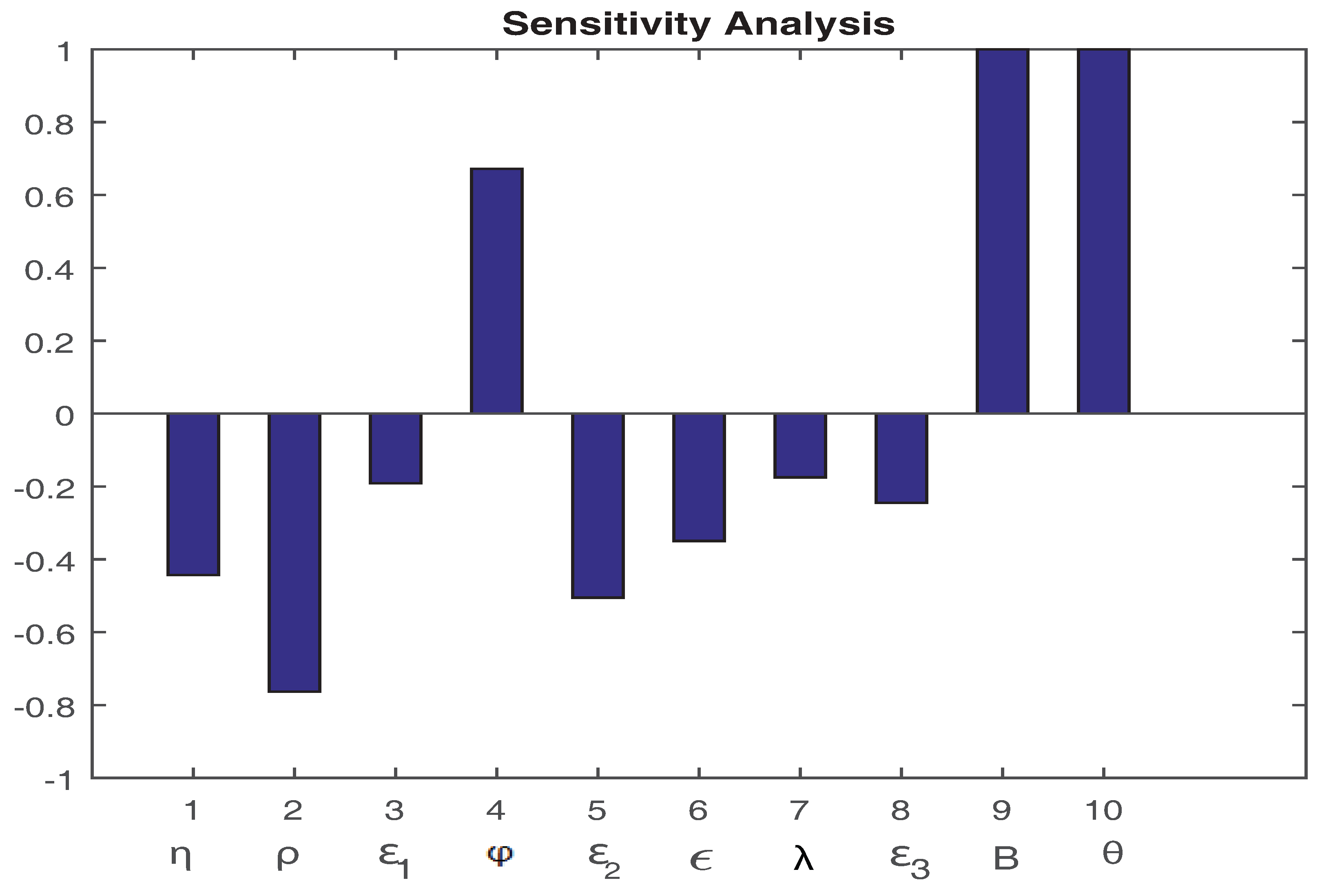
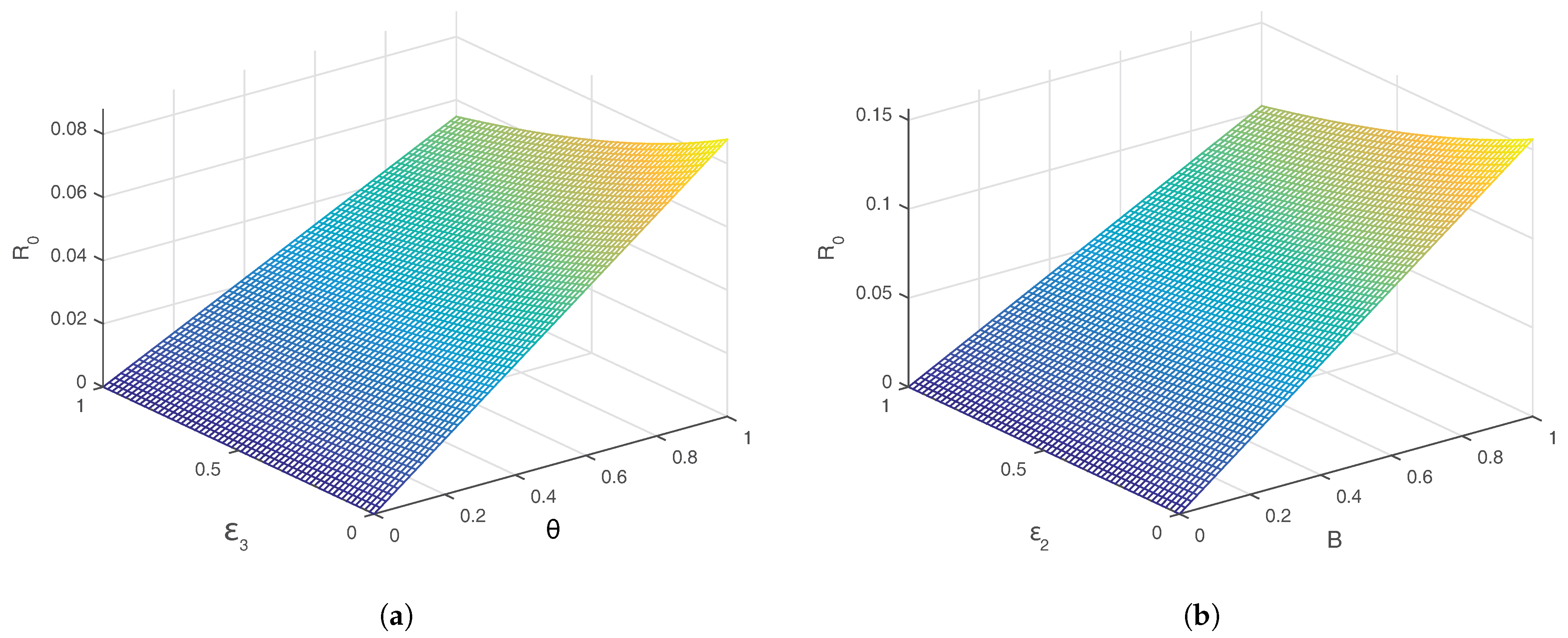
A vital tool for assessing how uncertain input parameters affect a system’s output is sensitivity analysis. Sensitivity indices can be computed using a variety of techniques, including direct differentiation, Latin hypercube sampling, and system linearization. In this study, the analytical expressions for the indices were provided using the direct differentiation method, allowing for a more thorough understanding of the behavior of the system. This study investigated the effects of various factors and gained a critical understanding of the comparative variability of the fundamental reproduction number, R 0 , and other parameters by applying this method to a COVID-19 model. These sensitivity indices provide policymakers and law enforcement agencies with useful data to create strategies that effectively combat COVID-19, and they are therefore essential in battling the pandemic. The graphical results are displayed in Figure 2 and Figure 3.

7. Numerical Scheme and Graphical Results

The Haar wavelet collocation method is a powerful numerical technique used for solving various types of differential equations. One of the main advantages of this method is its high accuracy, as it is capable of producing highly precise solutions for a wide range of problems. Additionally, the Haar wavelet collocation method is highly efficient, having a relatively low computational cost compared with other numerical methods. This is due to the compact support of the Haar wavelet, which allows for the use of fewer basis functions to represent the solution, resulting in faster calculations. Overall, the Haar wavelet collocation method is a reliable and efficient tool for numerical analysis, making it a popular choice among researchers and practitioners in various fields of science and engineering.
Consider the square integrable function space L 2 [ 0 , 1 ) , where S ˙ ( t ) , V ˙ ( t ) , E ˙ ( t ) , I ˙ ( t ) , Q ˙ ( t ) , and R ˙ ( t ) can be expressed as a Haar series, given by:
S ˙ ( t ) = m = 1 N α m ψ ˜ m ( t ) V ( t ) ˙ = m = 1 N γ m ψ ˜ m ( t ) E ( t ) ˙ = m = 1 N θ m ψ ˜ m ( t ) I ( t ) ˙ = m = 1 N λ m ψ ˜ m ( t ) , Q ( t ) ˙ = m = 1 N ϖ m ψ ˜ m ( t ) R ( t ) ˙ = m = 1 N σ m ψ ˜ m ( t ) .
Here, S ( 0 ) = S 0 represents the initial susceptible compartment, V ( 0 ) = V 0 represents the initial vaccinated compartment, E ( 0 ) = E 0 represents the initial exposed compartment, I ( 0 ) = I 0 represents the initial infected compartment, Q ( 0 ) = Q 0 represents the initial infected compartment, and R ( 0 ) = R 0 represents the initial recovered compartment. Integration of these equations leads to the following relation:
S ( t ) = S 0 + m = 1 N α m ϑ m , 1 ( t ) , V ( t ) = V 0 + m = 1 N γ m ϑ m , 1 ( t ) , E ( t ) = E 0 + m = 1 N θ m ϑ m , 1 ( t ) , I ( t ) = I 0 + m = 1 N λ m ϑ m , 1 ( t ) , Q ( t ) = Q 0 + m = 1 N ϖ m ϑ m , 1 ( t ) , R ( t ) = R 0 + m = 1 N σ m ϑ m , 1 ( t ) .
By using the Caputo derivative, we have
1 Γ ( n δ ) 0 t S ( n ) ( ϖ ) ( t ϖ ) n δ 1 d ϖ = B θ S ( t ) I ( t ) ( 1 + τ I ( t ) ) ( ε 1 + ρ + η ) S ( t ) + K V ( t ) , 1 Γ ( n δ ) 0 t V ( n ) ( ϖ ) ( t ϖ ) n δ 1 d ϖ = π S ( t ) ψ V ( t ) ( K + ρ ) V ( t ) , 1 Γ ( n δ ) 0 t E ( n ) ( ϖ ) ( t ϖ ) n δ 1 d ϖ = θ S ( t ) I ( t ) ( 1 + τ I ( t ) ) + ψ V ( t ) ( ε 2 + ρ + ) E ( t ) , 1 Γ ( n δ ) 0 t I ( n ) ( ϖ ) ( t ϖ ) n δ 1 d ϖ = φ E ( t ) ( λ + ϵ + ρ + ε 3 ) I ( t ) , 1 Γ ( n δ ) 0 t Q ( n ) ( ϖ ) ( t ϖ ) n δ 1 d ϖ = ε 1 S ( t ) + ε 2 E ( t ) + ε 3 I ( t ) + ( ρ + σ ) Q ( t ) , 1 Γ ( n δ ) 0 t R ( n ) ( ϖ ) ( t ϖ ) n δ 1 d ϖ = η S ( t ) + σ Q ( t ) + λ I ( t ) ρ R ( t ) .
As we have assumed that 0 < δ < 1 , therefore n = 1 , and we have
1 Γ ( 1 δ ) 0 t S ˙ ( t ) ( ϖ ) ( t ϖ ) δ d ϖ = B θ S ( t ) I ( t ) ( 1 + τ I ( t ) ) ( ε 1 + ρ + η ) S ( t ) + K V ( t ) , 1 Γ ( 1 δ ) 0 t V ( t ) ˙ ( ϖ ) ( t ϖ ) δ d ϖ = π S ( t ) ψ V ( t ) ( ρ + K ) V ( t ) , 1 Γ ( 1 δ ) 0 t E ( t ) ˙ ( ϖ ) ( t ϖ ) δ d ϖ = θ S ( t ) I ( t ) ( 1 + τ I ( t ) ) + ψ V ( t ) ( ε 2 + ρ + ) E ( t ) , 1 Γ ( 1 δ ) 0 t I ( t ) ˙ ( ϖ ) ( t ϖ ) δ d ϖ = φ E ( t ) ( λ + ϵ + ρ + ε 3 ) I ( t ) , 1 Γ ( 1 δ ) 0 t Q ( t ) ˙ ( ϖ ) ( t ϖ ) δ d ϖ = ε 1 S ( t ) + ε 2 E ( t ) + ε 3 I ( t ) ( ρ + σ ) Q ( t ) , 1 Γ ( 1 δ ) 0 t R ( t ) ˙ ( ϖ ) ( t ϖ ) δ d ϖ = η S ( t ) + σ Q ( t ) + λ I ( t ) ρ R ( t ) .
Haar approximations are used, and we have
1 Γ ( 1 δ ) 0 t m = 1 N α m ψ ˜ m ( ϖ ) ( t ϖ ) δ d ϖ = B θ I 0 + m = 1 N λ m ϑ m , 1 ( t ) S 0 + m = 1 N α m ϑ m , 1 ( t ) 1 + τ I 0 + m = 1 N λ m ϑ m , 1 ( t ) ( ε 1 + ρ + η ) S 0 + m = 1 N α m ϑ m , 1 ( t ) + K S 0 + m = 1 N γ m ϑ m , 1 ( t ) 1 Γ ( 1 δ ) 0 t m = 1 N γ m ψ ˜ m ( ϖ ) ( t ϖ ) δ d ϖ = π S 0 + m = 1 N α m ϑ m , 1 ( t ) ψ V 0 + m = 1 N γ m ϑ m , 1 ( t ) ( ρ + K ) V 0 + m = 1 N γ m ϑ m , 1 ( t ) 1 Γ ( 1 δ ) 0 t m = 1 N θ m ψ ˜ m ( ϖ ) ( t ϖ ) δ d ϖ = θ I 0 + m = 1 N λ m ϑ m , 1 ( t ) S 0 + m = 1 N α m ϑ m , 1 ( t ) + ψ V 0 + m = 1 N γ m ϑ m , 1 ( t ) 1 + τ I 0 + m = 1 N λ m ϑ m , 1 ( t ) ( ε 2 + ρ + φ ) E 0 + m = 1 N θ m ϑ m , 1 ( t ) 1 Γ ( 1 δ ) 0 t m = 1 N λ m ψ ˜ m ( ϖ ) ( t ϖ ) δ d ϖ = φ E 0 + m = 1 N θ m ϑ m , 1 ( t ) ( λ + ϵ + ρ + d 1 ) I 0 + m = 1 N λ m ϑ m , 1 ( t ) 1 Γ ( 1 δ ) 0 t m = 1 N ϖ m ψ ˜ m ( ϖ ) ( t ) δ d ϖ = ε 3 I ( t ) 0 + m = 1 N λ m ϑ m , 1 ( t ) + ε 2 E 0 + m = 1 N θ m ϑ m , 1 ( t ) + ε 1 S 0 + m = 1 N α m ϑ m , 1 ( t ) ( ρ + σ ) Q 0 + m = 1 N ϖ m ϑ m , 1 ( t ) 1 Γ ( 1 δ ) 0 t m = 1 N σ m ψ ˜ m ( ϖ ) ( t ϖ ) δ d ϖ = η S 0 + m = 1 N α m ϑ m , 1 ( t ) + σ Q 0 + m = 1 N σ m ϑ m , 1 ( t ) + λ I 0 + m = 1 N λ m ϑ m , 1 ( t ) + ρ R 0 + m = 1 N ζ m ϑ m , 1 ( t ) .
Upon simplification, we have
1 Γ ( 1 δ ) m = 1 N α m ψ ˜ m ( ϖ ) ( t ϖ ) δ d ϖ B + θ 1 + τ I 0 × I 0 S 0 + I 0 m = 1 N α m ϑ m , 1 ( t ) + S 0 m = 1 N θ m ϑ m , 1 ( t ) + m = 1 N α m ϑ m , 1 ( t ) m = 1 N θ m ϑ m , 1 ( t ) + θ I 0 S 0 τ m = 1 N θ m ϑ m , 1 ( t ) + I 0 τ m = 1 N α m ϑ m , 1 ( t ) m = 1 N θ m ϑ m , 1 ( t ) + S 0 τ m = 1 N θ m ϑ m , 1 ( t ) 2 + τ m = 1 N α m ϑ m , 1 ( t ) m = 1 N θ m ϑ m , 1 ( t ) 2 + ( ε 1 + ρ + η ) S 0 + ( ε 1 + ρ + η ) m = 1 N α m ϑ m , 1 ( t ) = 0 ,
1 Γ ( 1 δ ) 0 t m = 1 N γ m ψ ˜ m ( ϖ ) ( t ϖ ) δ d ϖ π S 0 + m = 1 N α m ϑ m , 1 ( t ) + ψ V 0 + m = 1 N γ m ϑ m , 1 ( t ) + ( ρ + K ) V 0 + m = 1 N γ m ϑ m , 1 ( t ) = 0 ,
1 Γ ( 1 δ ) m = 1 N θ m ψ ˜ m ( ϖ ) ( t ϖ ) δ d ϖ + θ 1 + τ I 0 × I 0 S 0 + I 0 m = 1 N α m ϑ m , 1 ( t ) + S 0 m = 1 N θ m ϑ m , 1 ( t ) + m = 1 N α m ϑ m , 1 ( t ) m = 1 N θ m ϑ m , 1 ( t ) + θ I 0 S 0 τ m = 1 N θ m ϑ m , 1 ( t ) + I 0 τ m = 1 N α m ϑ m , 1 ( t ) m = 1 N θ m ϑ m , 1 ( t ) + S 0 τ m = 1 N θ m ϑ m , 1 ( t ) 2 + τ m = 1 N α m ϑ m , 1 ( t ) m = 1 N θ m ϑ m , 1 ( t ) 2 + ( ε 2 + ρ + φ ) E 0 + ( ε 2 + ρ + φ ) m = 1 N θ m ϑ m , 1 ( t ) = 0 ,
1 Γ ( 1 δ ) 0 t m = 1 N λ m ψ ˜ m ( ϖ ) ( t ϖ ) δ d ϖ φ E 0 φ m = 1 N θ m ϑ m , 1 ( t ) + ( λ + ϵ + ρ + ε 3 ) I 0 + ( λ + ϵ + ρ + ε 3 ) m = 1 N λ m ϑ m , 1 ( t ) = 0 ,
1 Γ ( 1 δ ) 0 t m = 1 N ϖ m ψ ˜ m ( ϖ ) ( t ) δ d ϖ ε 3 I ( t ) 0 ε 3 m = 1 N λ m ϑ m , 1 ( t ) + ε 2 E 0 + ε 2 m = 1 N θ m ϑ m , 1 ( t ) + ε 1 S 0 + ε 1 m = 1 N α m ϑ m , 1 ( t ) + ( ρ + σ ) Q 0 + ( ρ + σ ) m = 1 N ϖ m ϑ m , 1 ( t ) = 0 ,
1 Γ ( 1 δ ) 0 t m = 1 N ζ m ψ ˜ m ( ϖ ) ( t ϖ ) δ d ϖ η S 0 S 0 m = 1 N α m ϑ m , 1 ( t ) σ Q 0 σ m = 1 N σ m ϑ m , 1 ( t ) λ I 0 λ m = 1 N λ m ϑ m , 1 ( t ) + ρ R 0 + ρ m = 1 N ζ m ϑ m , 1 ( t ) = 0 .
Using the method of Haar integration [52], the integral in the aforementioned system is approximately calculated as
ϰ κ f ( t ) d t κ ϰ N p = 1 N f t p = p = 1 N f ϰ + ( κ ϰ ) ( p 0.5 ) N
t N Γ ( 1 δ ) s = 1 N m = 1 N α m ψ ˜ m ϖ s t ϖ s δ B + θ 1 + τ I 0 × I 0 S 0 + I 0 m = 1 N α m ϑ m , 1 ( t ) + S 0 m = 1 N θ m ϑ m , 1 ( t ) + m = 1 N α m ϑ m , 1 ( t ) m = 1 N θ m ϑ m , 1 ( t ) + θ I 0 S 0 τ m = 1 N θ m ϑ m , 1 ( t ) + I 0 τ m = 1 N α m ϑ m , 1 ( t ) m = 1 N θ m ϑ m , 1 ( t ) + S 0 τ m = 1 N θ m ϑ m , 1 ( t ) 2 + τ m = 1 N α m ϑ m , 1 ( t ) m = 1 N θ m ϑ m , 1 ( t ) 2 + ( ε 1 + ρ + η ) S 0 + ( ε 1 + ρ + η ) m = 1 N α m ϑ m , 1 ( t ) = 0
1 N Γ ( 1 δ ) s = 1 N m = 1 N γ m ψ ˜ m ( ϖ ) ( t ϖ ) δ d ϖ π S 0 + m = 1 N α m ϑ m , 1 ( t ) + ψ V 0 + m = 1 N γ m ϑ m , 1 ( t ) + ( ρ + K ) V 0 + m = 1 N γ m ϑ m , 1 ( t ) = 0 ,
t N Γ ( 1 δ ) s = 1 N m = 1 N θ m ψ ˜ m ϖ s t ϖ s δ θ 1 + τ I 0 × I 0 S 0 + I 0 m = 1 N α m ϑ m , 1 ( t ) + S 0 m = 1 N θ m ϑ m , 1 ( t ) + m = 1 N α m ϑ m , 1 ( t ) m = 1 N θ m ϑ m , 1 ( t ) + θ I 0 S 0 τ m = 1 N θ m ϑ m , 1 ( t ) + I 0 τ m = 1 N α m ϑ m , 1 ( t ) m = 1 N θ m ϑ m , 1 ( t ) + S 0 τ m = 1 N θ m ϑ m , 1 ( t ) 2 + τ m = 1 N α m ϑ m , 1 ( t ) m = 1 N θ m ϑ m , 1 ( t ) 2 + ( ε 2 + ρ + φ ) E 0 + ( ε 2 + ρ + φ ) m = 1 N θ m ϑ m , 1 ( t ) = 0 ,
t N Γ ( 1 δ ) s = 1 N m = 1 N λ m ψ ˜ m ϖ s t ϖ s δ φ E 0 φ m = 1 N θ m ϑ m , 1 ( t ) + ( λ + ϵ + ρ + ε 3 ) I 0 + ( λ + ϵ + ρ + ε 3 ) m = 1 N λ m ϑ m , 1 ( t ) = 0 ,
t N Γ ( 1 δ ) s = 1 N m = 1 N ϖ m ψ ˜ m ϖ s t ϖ s δ ε 3 I 0 ε 3 m = 1 N λ m ϑ m , 1 ( t ) + ε 2 E ( t ) 0 + ε 2 m = 1 N θ m ϑ m , 1 ( t ) + ε 1 S 0 + ε 1 m = 1 N α m ϑ m , 1 ( t ) + ( ρ + σ ) Q 0 + ( ρ + σ ) m = 1 N ϖ m ϑ m , 1 ( t ) = 0 ,
t N Γ ( 1 δ ) s = 1 N m = 1 N ζ m ψ ˜ m ϖ s t ϖ s δ η S 0 S 0 m = 1 N α m ϑ m , 1 ( t ) σ Q 0 σ m = 1 N σ m ϑ m , 1 ( t ) λ I 0 λ m = 1 N λ m ϑ m , 1 ( t ) + ρ R 0 + ρ m = 1 N ζ m ϑ m , 1 ( t ) = 0 .
Let
Φ 1 , j = t N Γ ( 1 δ ) s = 1 N m = 1 N α m ψ ˜ m ϖ s t ϖ s δ B + θ 1 + τ I 0 × I 0 S 0 + I 0 m = 1 N α m ϑ m , 1 ( t ) + S 0 m = 1 N θ m ϑ m , 1 ( t ) + m = 1 N α m ϑ m , 1 ( t ) m = 1 N θ m ϑ m , 1 ( t ) + θ I 0 S 0 τ m = 1 N θ m ϑ m , 1 ( t ) + I 0 τ m = 1 N α m ϑ m , 1 ( t ) m = 1 N θ m ϑ m , 1 ( t ) + S 0 τ m = 1 N θ m ϑ m , 1 ( t ) 2 + τ m = 1 N α m ϑ m , 1 ( t ) m = 1 N θ m ϑ m , 1 ( t ) 2 + ( ε 1 + ρ + η ) S 0 + ( ε 1 + ρ + η ) m = 1 N α m ϑ m , 1 ( t ) .
Let
Φ 2 , j = 1 N Γ ( 1 δ ) s = 1 N m = 1 N γ m ψ ˜ m ( ϖ ) ( t ϖ ) δ d ϖ π S 0 + m = 1 N α m ϑ m , 1 ( t ) + ψ V 0 + m = 1 N γ m ϑ m , 1 ( t ) + ( ρ + K ) V 0 + m = 1 N γ m ϑ m , 1 ( t ) .
Let
Φ 3 , j = t N Γ ( 1 δ ) s = 1 N m = 1 N θ m ψ ˜ m ϖ s t ϖ s δ θ 1 + τ I 0 × I 0 S 0 + I 0 m = 1 N α m ϑ m , 1 ( t ) + S 0 m = 1 N θ m ϑ m , 1 ( t ) + m = 1 N α m ϑ m , 1 ( t ) m = 1 N θ m ϑ m , 1 ( t ) + θ I 0 S 0 τ m = 1 N θ m ϑ m , 1 ( t ) + I 0 τ m = 1 N α m ϑ m , 1 ( t ) m = 1 N θ m ϑ m , 1 ( t ) + S 0 τ m = 1 N θ m ϑ m , 1 ( t ) 2 + τ m = 1 N α m ϑ m , 1 ( t ) m = 1 N θ m ϑ m , 1 ( t ) 2 + ( ε 2 + ρ + φ ) E 0 + ( ε 2 + ρ + φ ) m = 1 N θ m ϑ m , 1 ( t ) .
Let
Φ 4 , j = t N Γ ( 1 δ ) s = 1 N m = 1 N λ m ψ ˜ m ϖ s t ϖ s δ φ E 0 φ m = 1 N θ m ϑ m , 1 ( t ) + ( λ + ϵ + ρ + ε 3 ) I 0 + ( λ + ϵ + ρ + ε 3 ) m = 1 N λ m ϑ m , 1 ( t ) .
Let
Φ 5 , j = t N Γ ( 1 δ ) s = 1 N m = 1 N ϖ m ψ ˜ m ϖ s t ϖ s δ ε 3 I 0 ε 3 m = 1 N λ m ϑ m , 1 ( t ) + ε 2 E ( t ) 0 + ε 2 m = 1 N θ m ϑ m , 1 ( t ) + ε 1 S 0 + ε 1 m = 1 N α m ϑ m , 1 ( t ) + ( ρ + σ ) Q 0 + ( ρ + σ ) m = 1 N ϖ m ϑ m , 1 ( t ) .
Let
Φ 6 , j = t N Γ ( 1 δ ) s = 1 N m = 1 N ζ m ψ ˜ m ϖ s t ϖ s δ η S 0 S 0 m = 1 N α m ϑ m , 1 ( t ) σ Q 0 σ m = 1 N σ m ϑ m , 1 ( t ) λ I 0 λ m = 1 N λ m ϑ m , 1 ( t ) + ρ R 0 + ρ m = 1 N ζ m ϑ m , 1 ( t ) .
The nodal points are placed to create the system of nonlinear algebraic equations shown below:
Φ 1 , j = t m N Γ ( 1 δ ) s = 1 N m = 1 N α m ψ ˜ m ϖ s t m ϖ s δ B + θ 1 + τ I 0 × I 0 S 0 + I 0 m = 1 N α m ϑ m , 1 ( t m ) + S 0 m = 1 N λ m ϑ m , 1 ( t m ) + m = 1 N α m ϑ m , 1 ( t m ) m = 1 N λ m ϑ m , 1 ( t m ) + θ I 0 S 0 τ m = 1 N λ m ϑ m , 1 ( t m ) + I 0 τ m = 1 N α m ϑ m , 1 ( t m ) m = 1 N λ m ϑ m , 1 ( t m ) + S 0 τ m = 1 N λ m ϑ m , 1 ( t m ) 2 + τ m = 1 N α m ϑ m , 1 ( t m ) m = 1 N λ m ϑ m , 1 ( t m ) 2 + ( ε 1 + ρ + η ) S 0 + ( ε 1 + ρ + η ) m = 1 N α m ϑ m , 1 ( t m ) ,
Φ 2 , j = 1 N Γ ( 1 δ ) s = 1 N m = 1 N γ m ψ ˜ m ( ϖ ) ( t m ϖ ) δ d ϖ π S 0 + m = 1 N α m ϑ m , 1 ( t m ) + ψ V 0 + m = 1 N γ m ϑ m , 1 ( t m ) + ( ρ + K ) V 0 + m = 1 N γ m ϑ m , 1 ( t m ) .
Φ 3 , j = t m N Γ ( 1 δ ) s = 1 N m = 1 N θ m ψ ˜ m ϖ s t m ϖ s δ B + θ 1 + τ I 0 × I 0 S 0 + I 0 m = 1 N α m ϑ m , 1 ( t m ) + S 0 m = 1 N λ m ϑ m , 1 ( t m ) + m = 1 N α m ϑ m , 1 ( t m ) m = 1 N λ m ϑ m , 1 ( t m ) + θ I 0 S 0 τ m = 1 N λ m ϑ m , 1 ( t m ) + I 0 τ m = 1 N α m ϑ m , 1 ( t m ) m = 1 N λ m ϑ m , 1 ( t m ) + S 0 τ m = 1 N λ m ϑ m , 1 ( t m ) 2 + τ m = 1 N α m ϑ m , 1 ( t m ) m = 1 N λ m ϑ m , 1 ( t m ) 2 + ψ V 0 + m = 1 N γ m ϑ m , 1 ( t m ) + ( ε 2 + ρ + φ ) m = 1 N θ m ϑ m , 1 ( t m ) ,
Φ 4 , j = t m N Γ ( 1 δ ) s = 1 N m = 1 N λ m ψ ˜ m ϖ s t m ϖ s δ φ E 0 φ m = 1 N θ m ϑ m , 1 ( t m ) + ( λ + ϵ + ρ + ε 3 ) I 0 + ( λ + ϵ + ρ + ε 3 ) m = 1 N λ m ϑ m , 1 ( t m ) .
Φ 5 , j = t m N Γ ( 1 δ ) s = 1 N m = 1 N ϖ m ψ ˜ m ϖ s t m ϖ s δ ε 3 I 0 ε 3 m = 1 N λ m ϑ m , 1 ( t m ) + ε 2 E 0 + ε 2 m = 1 N θ m ϑ m , 1 ( t m ) + ε 1 S 0 + ε 1 m = 1 N α m ϑ m , 1 ( t m ) + ( ρ + σ ) Q 0 + ( ρ + σ ) m = 1 N ϖ m ϑ m , 1 ( t m ) .
Let
Φ 6 , j = t m N Γ ( 1 δ ) s = 1 N m = 1 N ζ m ψ ˜ m ϖ s t m ϖ s δ η S 0 S 0 m = 1 N α m ϑ m , 1 ( t m ) σ Q 0 σ m = 1 N σ m ϑ m , 1 ( t m ) λ I 0 λ m = 1 N λ m ϑ m , 1 ( t m ) + ρ R 0 + ρ m = 1 N ζ m ϑ m , 1 ( t m ) .
Using Broyden’s approach, this system is resolved. The Jacobian is given by
J = J j p 6 N × 6 N
where
Φ 1 , j α m = t m N Γ ( 1 δ ) s = 1 N m = 1 N ψ ˜ m ϖ s t m ϖ s δ + θ 1 + τ I 0 × + I 0 m = 1 N ϑ m , 1 ( t m ) + m = 1 N ϑ m , 1 ( t m ) m = 1 N θ m ϑ m , 1 ( t m ) + θ + I 0 τ m = 1 N ϑ m , 1 ( t m ) m = 1 N λ m ϑ m , 1 ( t m ) + τ m = 1 N ϑ m , 1 ( t m ) m = 1 N λ m ϑ m , 1 ( t m ) 2 + ( ε 1 + ρ + η ) m = 1 N ϑ m , 1 ( t m ) Φ 1 , j γ m = m = 1 N ϑ m , 1 ( t m ) , Φ 1 , j θ m = 0 , Φ 1 , j ϖ m = 0 , Φ 1 , j σ m = 0 , Φ 1 , j λ m = θ 1 + τ I 0 × S 0 m = 1 N ϑ m , 1 ( t m ) + m = 1 N α m ϑ m , 1 ( t m ) m = 1 N ϑ m , 1 ( t m ) + θ I 0 S 0 τ m = 1 N ϑ m , 1 ( t m ) + I 0 τ m = 1 N α m ϑ m , 1 ( t m ) m = 1 N ϑ m , 1 ( t m ) + 2 λ m S 0 τ m = 1 N ϑ m , 1 ( t m ) 2 + τ m = 1 N α m ϑ m , 1 ( t m ) m = 1 N ϑ m , 1 ( t m ) 2 ,
Φ 2 , j α m = π m = 1 N α m ϑ m , 1 ( t m ) , Φ 2 , j θ m = 0 , Φ 2 , j λ m = 0 , Φ 1 , j ϖ m = 0 , Φ 1 , j σ m = 0 , Φ 2 , j γ m = 1 N Γ ( 1 δ ) s = 1 N m = 1 N γ m ψ ˜ m ( ϖ ) ( t m ϖ ) δ d ϖ + ψ V 0 + m = 1 N ϑ m , 1 ( t m ) + ( ρ + K ) V 0 + m = 1 N ϑ m , 1 ( t m ) .
Φ 3 , j α m = θ 1 + τ I 0 × + I 0 m = 1 N ϑ m , 1 ( t m ) + m = 1 N ϑ m , 1 ( t m ) m = 1 N θ m ϑ m , 1 ( t m ) + θ + I 0 τ m = 1 N ϑ m , 1 ( t m ) m = 1 N λ m ϑ m , 1 ( t m ) + τ m = 1 N ϑ m , 1 ( t m ) m = 1 N λ m ϑ m , 1 ( t m ) 2 Φ 3 , j γ m = m = 1 N ϑ m , 1 ( t m ) , Φ 3 , j θ m = t m N Γ ( 1 δ ) s = 1 N m = 1 N ψ ˜ m ϖ s t m ϖ s δ + ( ε 2 + ρ + φ ) m = 1 N ϑ m , 1 ( t m ) , Φ 3 , j ϖ m = 0 , Φ 3 , j σ m = 0 , Φ 3 , j λ m = θ 1 + τ I 0 × S 0 m = 1 N ϑ m , 1 ( t m ) + m = 1 N α m ϑ m , 1 ( t m ) m = 1 N ϑ m , 1 ( t m ) + θ I 0 S 0 τ m = 1 N ϑ m , 1 ( t m ) + I 0 τ m = 1 N α m ϑ m , 1 ( t m ) m = 1 N ϑ m , 1 ( t m ) + 2 λ m S 0 τ m = 1 N ϑ m , 1 ( t m ) 2 + τ m = 1 N α m ϑ m , 1 ( t m ) m = 1 N ϑ m , 1 ( t m ) 2 ,
Φ 4 , j α m = 0 , Φ 4 , j γ m = 0 , Φ 4 , j ϖ m = 0 , Φ 4 , j σ m = 0 , Φ 4 , j θ m = φ m = 1 N θ m ϑ m , 1 ( t m ) , Φ 4 , j λ m = t m N Γ ( 1 δ ) s = 1 N m = 1 N ψ ˜ m ϖ s t m ϖ s δ ( λ + ϵ + ρ + ε 3 ) m = 1 N ϑ m , 1 ( t m ) .
Φ 5 , j α m = ε 1 m = 1 N ϑ m , 1 ( t m ) , Φ 5 , j γ m = 0 , Φ 5 , j ϖ m = t m N Γ ( 1 δ ) s = 1 N m = 1 N ϖ m ψ ˜ m ϖ s t m ϖ s δ , + ( ρ + σ ) m = 1 N ϖ m ϑ m , 1 ( t m ) Φ 5 , j σ m = 0 , Φ 5 , j θ m = ε 2 m = 1 N θ m ϑ m , 1 ( t m ) , Φ 5 , j λ m = ε 3 m = 1 N ϑ m , 1 ( t m ) .
Φ 6 , j α m = S 0 m = 1 N ϑ m , 1 ( t m ) , Φ 6 , j γ m = 0 , Φ 6 , j ϖ m = t m N Γ ( 1 δ ) s = 1 N m = 1 N ψ ˜ m ϖ s t m ϖ s δ , + ( ρ + σ ) m = 1 N ϑ m , 1 ( t m ) Φ 6 , j θ m = 0 , Φ 6 , j λ m = λ m = 1 N λ m ϑ m , 1 ( t m ) . Φ 6 , j σ m = t m N Γ ( 1 δ ) s = 1 N m = 1 N ψ ˜ m ϖ s t m ϖ s δ σ m = 1 N σ m ϑ m , 1 ( t m ) + ρ m = 1 N ϑ m , 1 ( t m ) .
This system’s solution yields the values of α m ’s, γ m ’s, λ m ’s, ϖ m ’s, and σ m ’s unknown coefficients. By entering α m ’s, γ m ’s, λ m ’s, ϖ m ’s, and σ m ’s unknown coefficients into Equation (29), it is possible to calculate the necessary solutions S ( t ) , V ( t ) , E ( t ) , I ( t ) , Q ( t ) , and R ( t ) at nodal locations. The experimental rate of convergence, denoted by the formula r ϱ ( N ) [53], can be calculated as follows:
r ϱ ( N ) = 1 log 2 log Maximum absolute error at N 2 Maximum absolute error at N .

Graphical Results

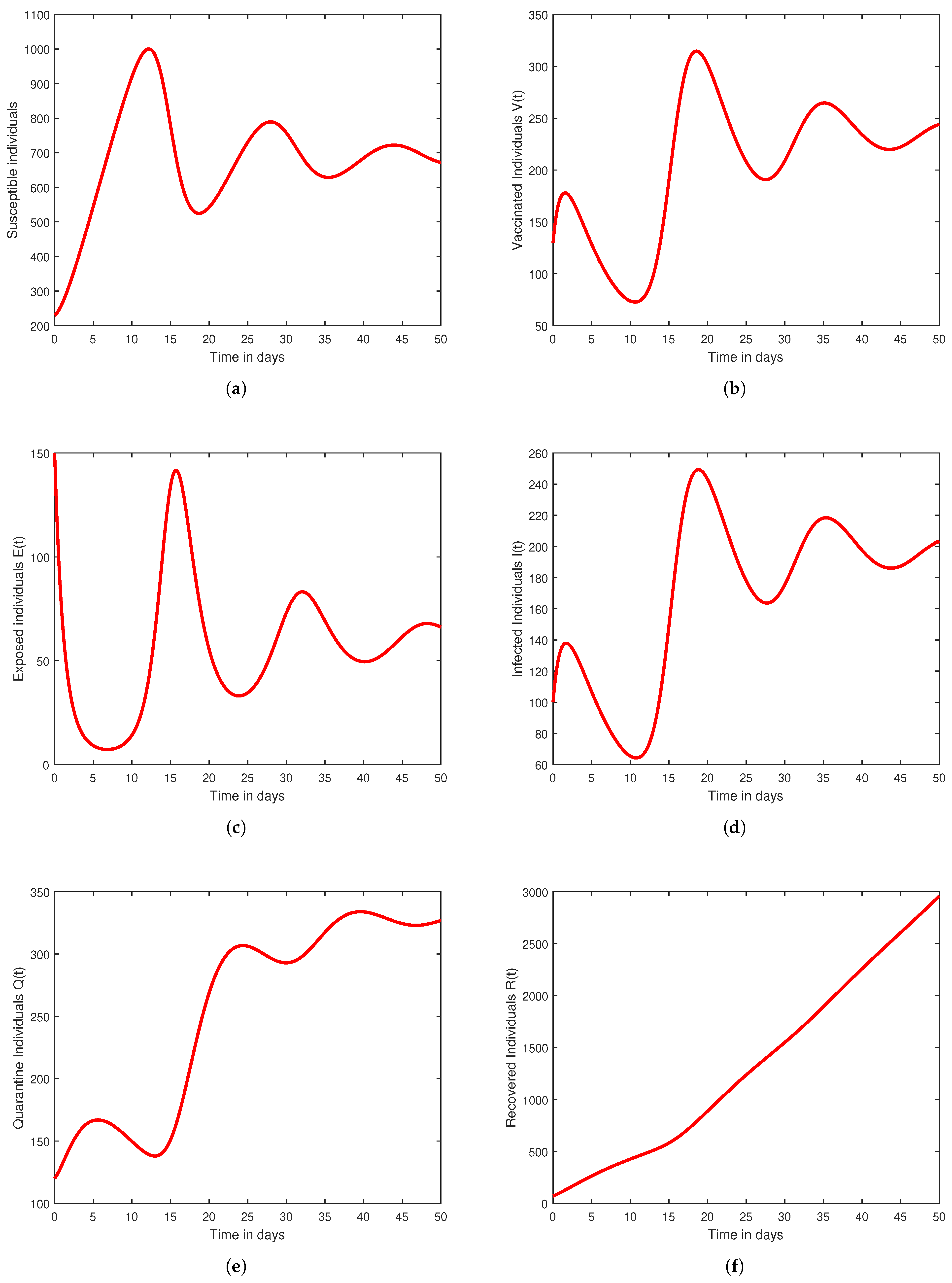
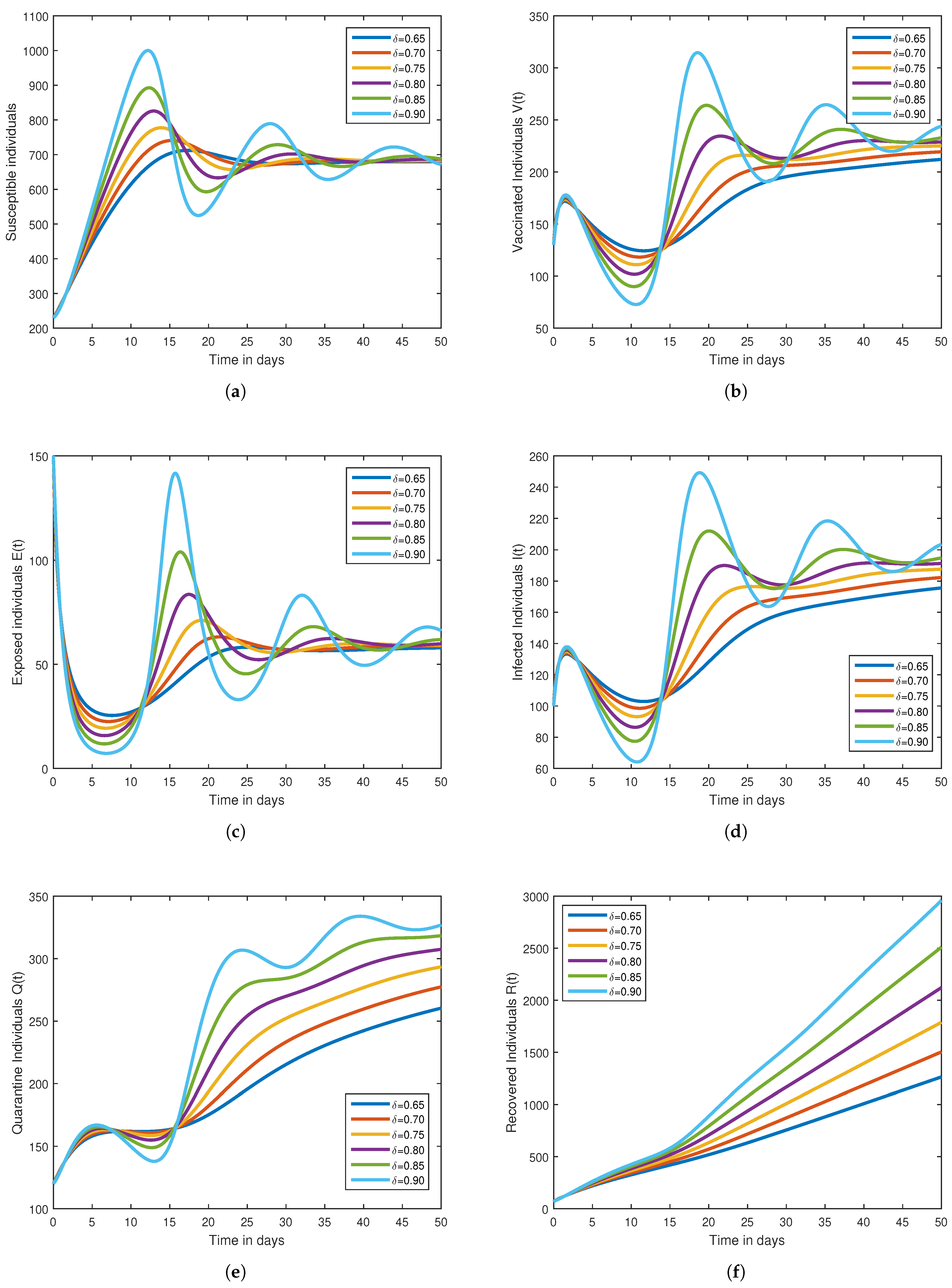
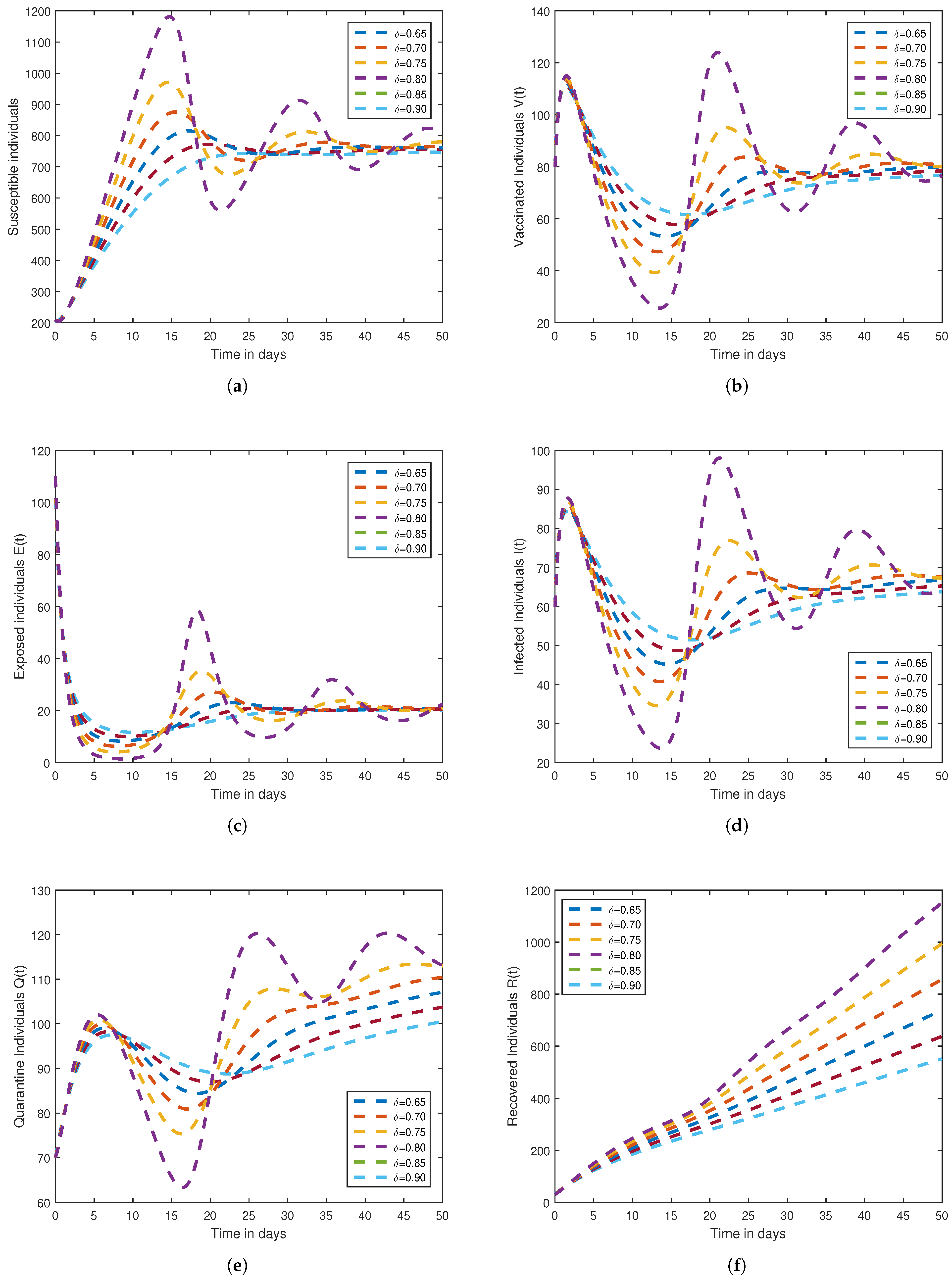
This section presents graphical results for the fractional-order model (14). The fractional model was numerically solved based on the method outlined in [47,54] and using the information from Table 1. The resulting figures, namely Figure 4, Figure 5, Figure 6 and Figure 7, illustrate the dynamics of the susceptible S ( t ) , vaccinated V ( t ) , exposed E ( t ) , infected I ( t ) , quarantined Q ( t ) , and recovered R ( t ) individuals. Figure 5a shows that susceptible individuals are characterized by fractional-order derivatives ranging between 0.55 and 0.95 , and as time progresses, the number of susceptible individuals decreases due to exposure to the virus. This behavior is expected and observed in other epidemiological models. The population of vaccinated individuals is shown in Figure 5b, and it grows both steadily and quickly as the fractional-order derivative approaches its classical counterpart. Similarly, the population of exposed individuals is shown in Figure 5c, and it greatly decreases in the first 15 days while both steadily and quickly increasing as the fractional-order derivative approaches its classical counterpart. This increase is brought on by more susceptible people becoming infected during the first few weeks of the outbreak and joining the exposed class. An increased risk of transmission during the early stages of the epidemic may be indicated by the rise in exposed individuals. Figure 5c displays the number of infected people, which rises as the fractional order gets closer to one. The fractional order, which becomes more sensitive as it gets closer to one, is what is causing this increase. Within a few weeks of exposure, the majority of people in the quarantined and infectious stages of the infection leave the exposed class. Figure 5d illustrates the dynamics of the quarantined individuals, who exhibit a similar behavior as the exposed population. The population of exposed individuals increases as the fractional-order derivative approaches the integer order. Figure 5e shows how the fractional order affects the number of recovered individuals, which grows steadily as the fractional-order derivative approaches the classical value. This is due to the infected individuals recovering, which aids in disease containment. Raising the fractional order can cause the population of the recovered class to grow considerably more quickly. These results suggest that the exposed population is similarly affected by the fractional order regardless of the strain of infection.

8. Conclusions

The S V E I Q R COVID-19 epidemic model under fractional derivatives in the Caputo sense has been studied in this article. Some findings from fixed point theory are taken into consideration when determining the existence and uniqueness of the proposed model. This study simulates the spread of the COVID-19 Omicron variant in Pakistan using fractional-order models and the Haar wavelet collocation method. The study makes use of actual data from Pakistan, which improves the model’s precision and applicability. To determine the factors that most influence the spread of the virus, a sensitivity analysis was also carried out. This study sheds light on the dynamics of the pandemic and emphasizes the significance of taking fractional order into account when modeling infectious diseases. In terms of future directions, this study can be extended to incorporate additional elements such as vaccination rates, travel restrictions, and socio-economic conditions. To evaluate the efficacy of various intervention strategies and compare the effects of various COVID-19 variants, the model can also be applied to other regions or nations. Additionally, this study can be expanded to assess the effects of various compliance levels with public health measures, such as mask use and social distancing. To determine the most effective and precise method, this study can be expanded to compare the performance of various numerical solution techniques for fractional-order models.

Author Contributions

Conceptualization, R.Z.; Software, Z.R.; Formal analysis, R.Z.; Investigation, Z.R.; Writing—original draft, R.Z.; Supervision, Z.R.; Project administration, Z.R. All authors have read and agreed to the published version of the manuscript.

Funding

The authors extend their appreciation to the Ministry of Education in KSA for funding this research work through project number KKU-IFP2-H-9.

Data Availability Statement

Data sharing is not applicable to this article, as no data sets were generated during the current study.

Acknowledgments

The acknowledgement to the Ministry of Education of the Kingdom of Saudi Arabia for the funding of this research work by project number KKU-IFP2-H-9.

Conflicts of Interest

The authors declare no conflict of interest.

References

  1. Omrani, A.S.; Al-Tawfiq, J.A.; Memish, Z.A. Middle East respiratory syndrome coronavirus (MERS-CoV): Animal to human interaction. Pathog. Glob. Health 2015, 109, 354–362. [Google Scholar] [CrossRef]
  2. World Health Organization. Weekly Epidemiological Update on COVID-19—11 January 2023. Available online: https://www.who.int/publications/m/item/weekly-epidemiological-update-on-covid-19---11-january-2023 (accessed on 11 January 2023).
  3. Tay, M.Z.; Poh, C.M.; Rénia, L.; MacAry, P.A.; Ng, L.F. The trinity of COVID-19: Immunity, inflammation and intervention. Nat. Rev. Immunol. 2020, 20, 363–374. [Google Scholar] [CrossRef] [PubMed]
  4. Backer, J.A.; Klinkenberg, D.; Wallinga, J. Incubation period of 2019 novel coronavirus (2019-nCoV) infections among travellers from Wuhan, China, 20–28 January 2020. Eurosurveillance 2020, 25, 2000062. [Google Scholar] [CrossRef] [PubMed]
  5. Kronbichler, A.; Kresse, D.; Yoon, S.; Lee, K.H.; Effenberger, M.; Shin, J.I. Asymptomatic patients as a source of COVID-19 infections: A systematic review and meta-analysis. Int. J. Infect. Dis. 2020, 98, 180–186. [Google Scholar] [CrossRef]
  6. Khan, A.; Zarin, R.; Hussain, G.; Ahmad, N.A.; Mohd, M.H.; Yusuf, A. Stability analysis and optimal control of covid-19 with convex incidence rate in Khyber Pakhtunkhawa (Pakistan). Results Phys. 2021, 20, 103703. [Google Scholar] [CrossRef]
  7. Khan, A.; Zarin, R.; Akgul, A.; Saeed, A.; Gul, T. Fractional optimal control of COVID-19 pandemic model with generalized Mittag-Leffler function. Adv. Differ. Equ. 2021, 2021, 387. [Google Scholar] [CrossRef]
  8. Alqarni, M.S.; Alghamdi, M.; Muhammad, T.; Alshomrani, A.S.; Khan, M.A. Mathematical modeling for novel coronavirus (COVID-19) and control. Numer. Methods Partial. Differ. Equ. 2022, 38, 760–776. [Google Scholar] [CrossRef] [PubMed]
  9. Khan, A.; Zarin, R.; Khan, S.; Saeed, A.; Gul, T.; Humphries, U.W. Fractional dynamics and stability analysis of COVID-19 pandemic model under the harmonic mean type incidence rate. Comput. Methods Biomech. Biomed. Eng. 2022, 25, 619–640. [Google Scholar] [CrossRef]
  10. Kucharski, A.J.; Russell, T.W.; Diamond, C.; Liu, Y.; Edmunds, J.; Funk, S.; Eggo, R.M. Early dynamics of transmission and control of COVID-19: A mathematical modelling study. Lancet Infect. Dis. 2020, 20, 553–558. [Google Scholar] [CrossRef]
  11. Ferguson, N.M.; Laydon, D.; Nedjati-Gilani, G.; Imai, N.; Ainslie, K.; Baguelin, M.; Bhatia, S.; Boonyasiri, A.; Cucunuba, Z.; Cuomo-Dannenburg, G.; et al. Impact of Non-Pharmaceutical Interventions (NPIs) to Reduce COVID-19 Mortality and Healthcare Demand. Imperial College COVID-19 Response Team. 2020. Available online: https://www.imperial.ac.uk/media/imperial-college/medicine/sph/ide/gida-fellowships/Imperial-College-COVID19-NPI-modelling-16-03-2020.pdf (accessed on 16 March 2020).
  12. Marathe, A.; Lewis, B.; Chen, J. COVID-19: Understanding the spread of infectious diseases. Nat. Rev. Phys. 2020, 2, 447–456. [Google Scholar]
  13. Hethcote, H.W.; Shuai, Z.; Van den Driessche, P. COVID-19 transmission dynamics in the United States: A mathematical model with a realistic age structure. Math. Biosci. Eng. 2021, 18, 2672–2690. [Google Scholar] [CrossRef]
  14. Yopadhyay, A.; Nabar, N.R.; Salathé, M. A review of data-driven epidemiological models of infectious diseases. In Global Dynamics of Infectious Diseases: Impact of Social Heterogeneity; Springer: Berlin, Germany, 2021; pp. 19–41. [Google Scholar]
  15. Liu, P.; Huang, X.; Zarin, R.; Cui, T.; Din, A. Modeling and numerical analysis of a fractional order model for dual variants of SARS-CoV-2. Alex. Eng. J. 2023, 65, 427–442. [Google Scholar] [CrossRef]
  16. Daniloski, Z.; Guo, X.; Sanjana, N.E. The D614G mutation in SARS-CoV-2 spike increases transduction of multiple human cell types. Nat. Commun. 2021, 12, 1–9. [Google Scholar] [CrossRef]
  17. Saberi, M.; Moshksayan, K.; Barati, M.; Soleymani, F.; Eftekhari, P. Modeling and analysis of COVID-19 infection dynamics with fractional-order derivatives. Chaos Solitons Fractals 2021, 146, 110844. [Google Scholar]
  18. Goyal, M.; Baskonus, H.M.; Prakash, A. An efficient technique for a time fractional model of lassa hemorrhagic fever spreading in pregnant women. Eur. Phys. J. Plus 2019, 134, 482. [Google Scholar] [CrossRef]
  19. Gao, W.; Veeresha, P.; Prakasha, D.G.; Baskonus, H.M.; Yel, G. New approach for the model describing the deathly disease in pregnant women using Mittag-Leffler function. Chaos Solitons Fractals 2020, 134, 109696. [Google Scholar] [CrossRef]
  20. Alqahtani, R.T.; Ahmad, S.; Akgül, A. Dynamical analysis of bio-ethanol production model under generalized nonlocal operator in Caputo sense. Mathematics 2021, 9, 2370. [Google Scholar] [CrossRef]
  21. Agarwal, P.; Singh, R. Modelling of transmission dynamics of Nipah virus (Niv): A fractional order approach. Phys. A Stat. Mech. Its Appl. 2020, 547, 124243. [Google Scholar] [CrossRef]
  22. Zarin, R.; Khan, A.; Yusuf, A.; Abdel-Khalek, S.; Mustafa Inc. Analysis of fractional COVID-19 epidemic model under Caputo operator. Math. Methods Appl. Sci. 2021, 6, 115–122. [Google Scholar] [CrossRef]
  23. Zarin, R.; Khan, A.; Kumar, P. Fractional-order dynamics of Chagas-HIV epidemic model with different fractional operators. AIMS Math. 2022, 7, 18897–18924. [Google Scholar] [CrossRef]
  24. Baleanu, D.; Fernez, A.; Akgül, A. On a fractional operator combining proportional and classical differintegrals. Mathematics 2020, 8, 360. [Google Scholar] [CrossRef]
  25. Caputo, M.; Fabrizio, M. A new definition of fractional derivative without singular kernel. Prog. Fract. Differ. Appl. 2015, 1, 73–85. [Google Scholar]
  26. Atangana, A.; Baleanu, D. New fractional derivatives with nonlocal and non-singular kernel: Theory and application to heat transfer model. arXiv 2016, arXiv:1602.03408. [Google Scholar] [CrossRef]
  27. Andrew, O.; Abbas, M.; Abdel-Aty, A.-H. Assessing the impact of SARS-CoV-2 infection on the dynamics of dengue and HIV via fractional derivatives. Chaos Solitons Fractals 2022, 162, 112427. [Google Scholar]
  28. Omame, A.; Abbas, M.; Onyenegecha, C.P. Backward bifurcation and optimal control in a co-infection model for SARS-CoV-2 and ZIKV. Results Phys. 2022, 37, 105481. [Google Scholar] [CrossRef]
  29. Agarwal, P.; Choi, J.; Paris, R.B. Extended Riemann-Liouville fractional derivative operator and its applications. J. Nonlinear Sci. Appl. (JNSA) 2015, 8, 451–466. [Google Scholar] [CrossRef]
  30. Zarin, R.; Khan, A.; Inc, M.; Humphries, U.W.; Karite, T. Dynamics of five grade leishmania epidemic model using fractional operator with Mittag–Leffler kernel. Chaos Solitons Fractals 2021, 147, 110985. [Google Scholar] [CrossRef]
  31. Agarwal, P.; Choi, J. Fractional calculus operators and their image formulas. J. Korean Math. Soc. 2016, 53, 1183–1210. [Google Scholar] [CrossRef]
  32. Atangana, A. Non validity of index law in fractional calculus: A fractional differential operator with Markovian and non-Markovian properties. Phys. A Stat. Mech. Its Appl. 2018, 505, 688–706. [Google Scholar] [CrossRef]
  33. Zarin, R. Modeling and numerical analysis of fractional order hepatitis B virus model with harmonic mean type incidence rate. Comput. Methods Biomech. Biomed. Eng. 2022, 1–16. [Google Scholar] [CrossRef] [PubMed]
  34. Zarin, R.; Ahmed, I.; Kumam, P.; Zeb, A.; Din, A. Fractional modeling and optimal control analysis of rabies virus under the convex incidence rate. Results Phys. 2021, 28, 104665. [Google Scholar] [CrossRef]
  35. Ahmad, S.; Ullah, A.; Akgül, A.; Baleanu, D. Analysis of the fractional tumour-immune-vitamins model with Mittag–Leffler kernel. Results Phys. 2020, 19, 103559. [Google Scholar] [CrossRef]
  36. Atangana, A. A novel Covid-19 model with fractional differential operators with singular and non-singular kernels: Analysis and numerical scheme based on Newton polynomial. Alexandria Eng. J. 2021, 60, 3781–3806. [Google Scholar] [CrossRef]
  37. Bansal, K.; Arora, S.; Pritam, K.S.; Mathur, T.; Agarwal, S. Dynamics of Crime Transmission Using Fractional-Order Differential Equations. Fractals 2022, 30, 2250012. [Google Scholar] [CrossRef]
  38. Pritam, K.S.; Mathur, T.; Agarwal, S. Underlying dynamics of crime transmission with memory. Chaos Solitons Fractals 2021, 146, 110838. [Google Scholar] [CrossRef]
  39. Rahman, M.U.; Ahmad, S.; Arfan, M.; Akgül, A.; Jarad, F. Fractional Order Mathematical Model of Serial Killing with Different Choices of Control Strategy. Fractal Fract. 2022, 6, 162. [Google Scholar] [CrossRef]
  40. Zhi, S.; Deng, L.-Y.; Qing, J.C. Numerical Solution of Differential Equations by Using Haar Wavelets. In Proceedings of the International Conference on Wavelet Analysis and Pattern Recognition, Beijing, China, 2–4 November 2007; pp. 1039–1044. [Google Scholar]
  41. Shah, K.; Khan, Z.A.; Ali, A.; Amin, R.; Khan, H.; Khan, A. Haar wavelet collocation approach for the solution of fractional order COVID-19 model using Caputo derivative. Alex. Eng. J. 2020, 59, 3221–3231. [Google Scholar] [CrossRef]
  42. Prakash, B.; Setia, A.; Alapatt, D. Numerical solution of nonlinear fractional SEIR epidemic model by using Haar wavelets. J. Comput. Sci. 2017, 22, 109–118. [Google Scholar] [CrossRef]
  43. Kumar, D.; Singh, J.; Baleanu, D. A new analysis of the Fornberg-Whitham equation pertaining to a fractional derivative with Mittag-Leffler-type kernel. Eur. Phys. J. Plus 2018, 133, 70. [Google Scholar] [CrossRef]
  44. Kumar, D.; Singh, J.; Purohit, S.D.; Swroop, R. A hybrid analytical algorithm for nonlinear fractional wave-like equations. Math. Model. Nat. Phenom. 2019, 14, 304. [Google Scholar] [CrossRef]
  45. Caputo, M.; Mainardi, F. A new dissipation model based on memory mechanism. Pure Appl. Geophys. 1971, 91, 134–147. [Google Scholar] [CrossRef]
  46. Chen, Y.; Yi, M.; Yu, C. Error analysis for numerical solution of fractional differential equation by Haar wavelets method. J. Comput. Sci. 2012, 3, 367–373. [Google Scholar] [CrossRef]
  47. Lepik, Ü.; Hein, H. Haar wavelets. In Haar Wavelets; Springer: Cham, Switzerland, 2014; pp. 7–20. [Google Scholar]
  48. Van den Driessche, P.; Watmough, J. Reproduction number and sub-threshold endemic equilbria for compartmental models of disease transmission. Math. Biosci. 2002, 180, 29–38. [Google Scholar] [CrossRef]
  49. Taylor, A.E.; Lay, D.C. Introduction to Functional Analysis; Wiley: New York, NY, USA, 1958; Volume 1. [Google Scholar]
  50. Available online: https://www.who.int/countries/pak/ (accessed on 23 August 2022).
  51. Mandal, M.; Jana, S.; Nandi, S.K.; Khatua, A.; Adak, S.; Kar, T.K. A model based study on the dynamics of COVID-19: Prediction and control. Chaos Solitons Fractals 2020, 136, 109889. [Google Scholar] [CrossRef]
  52. Li, Y.; Zhao, W. Haar wavelet operational matrix of fractional order integration and its applications in solving the fractional order differential equations. Appl. Math. Comp. 2010, 216, 2276–2285. [Google Scholar] [CrossRef]
  53. Majak, J.; Shvartsman, B.; Karjust, K.; Mikola, M.; Haavajõe, A.; Pohlak, M. On the accuracy of the Haar wavelet discretization method. Compos. Part B Eng. 2015, 80, 321–327. [Google Scholar] [CrossRef]
  54. Zarin, R.; Khaliq, H.; Khan, A.; Ahmed, I.; Humphries, U.W. A Numerical Study Based on Haar Wavelet Collocation Methods of Fractional-Order Antidotal Computer Virus Model. Symmetry 2023, 15, 621. [Google Scholar] [CrossRef]
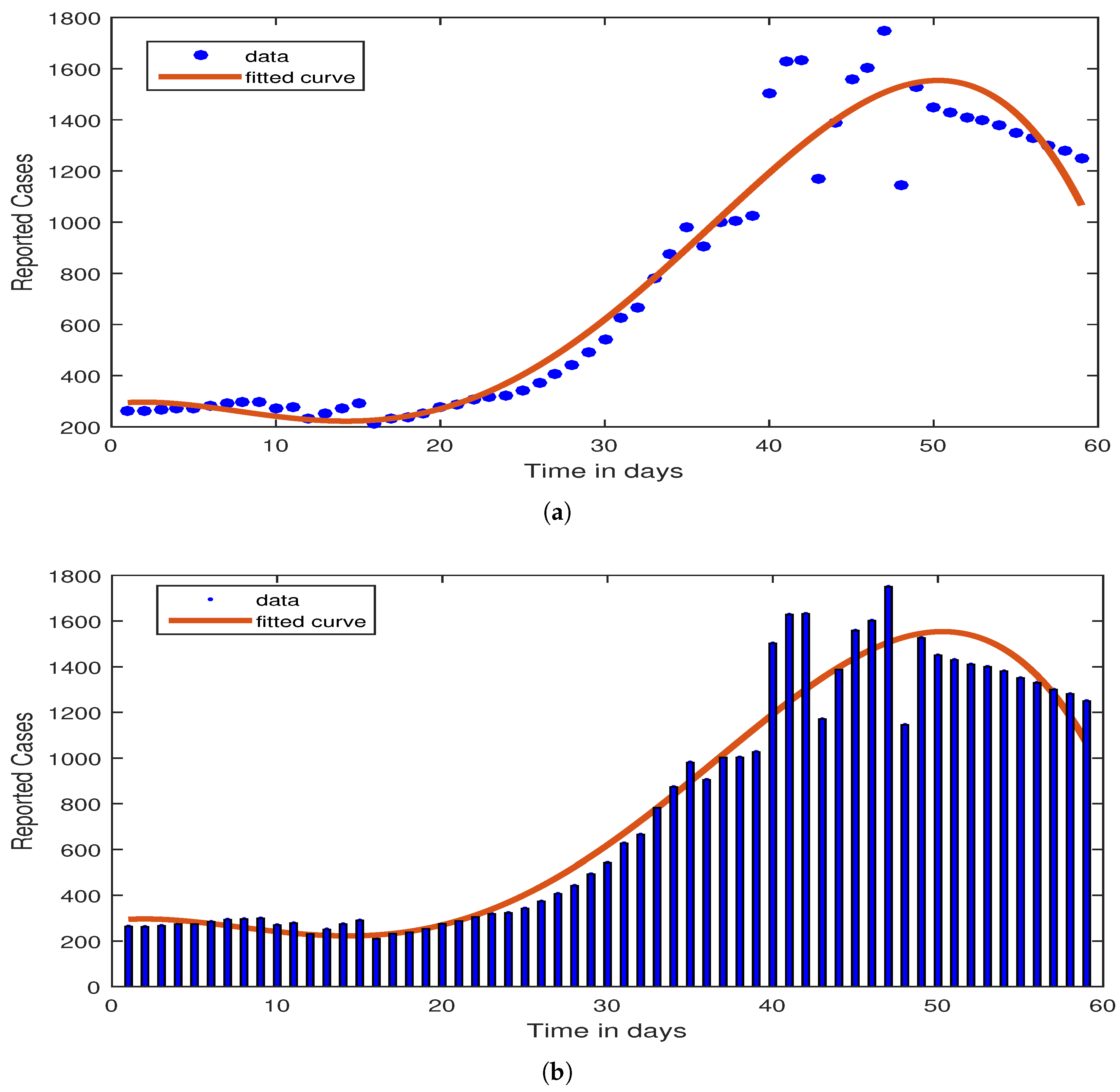
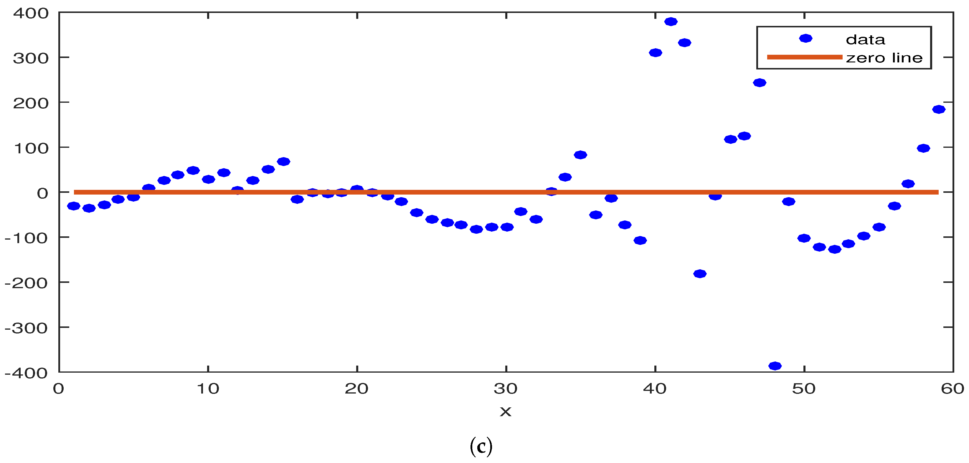
Figure 1. The figure illustrates the profiles of the best-fitted curve and its corresponding residuals for the daily cumulative cases of COVID-19 in Pakistan from 23 Jun 2022 to 23 August 2022. Furthermore, the figures (a,b) represent the model fit with reported infected cases and (c) represents the residuals.
Mathematics 11 01925 g001aMathematics 11 01925 g001b
Figure 2. Global sensitivity.
Mathematics 11 01925 g002
Figure 3. Sensitivity of various parameters vs. R 0 are displayed in (ae).
Mathematics 11 01925 g003aMathematics 11 01925 g003b
Figure 4. The caputo version of the fractional model’s behavior for each state variable is depicted in the figure at δ = 0.95 . Furthermore, the figures (af) represents susceptible people S ( t ) , vaccinated people V ( t ) , exposed people E ( t ) , infectious people I ( t ) , quarantined people Q ( t ) , and recovered people R ( t ) .
Mathematics 11 01925 g004
Figure 5. The caputo version of the fractional model’s behavior for each state variable is depicted using the parameter values in the figure. Furthermore, the figures (af) represents susceptible people S ( t ) , vaccinated people V ( t ) , exposed people E ( t ) , infectious people I ( t ) , quarantined people Q ( t ) , and recovered people R ( t ) .
Mathematics 11 01925 g005
Figure 6. The behavior of each state variable for the Caputo fractional model utilizing a different set of initial conditions is depicted in the figure. Furthermore, the figures (af) represents susceptible people S ( t ) , vaccinated people V ( t ) , exposed people E ( t ) , infectious people I ( t ) , quarantined people Q ( t ) , and recovered people R ( t ) .
Mathematics 11 01925 g006
Figure 7. The behavior of each state variable is depicted in the figure for θ = 0.01815 . Furthermore, the figures (af) represents susceptible people S ( t ) , vaccinated people V ( t ) , exposed people E ( t ) , infectious people I ( t ) , quarantined people Q ( t ) , and recovered people R ( t ) .
Mathematics 11 01925 g007
Table 1. The table contains descriptions and estimated values for the parameters.
Symbol of ParametersValues of ParametersReferences
B 50.4057 [51]
θ 0.0019 Estimated
τ 0.0205 Estimated
ϵ 0.1571 Estimated
ε 1 0.01772 Estimated
ε 2 0.0805 Estimated
ε 3 0.0876 Estimated
ρ 0.0205 [51]
η 0.1460 Estimated
α 0.3506 Estimated
K 0.1530 Estimated
σ 0.0059 Estimated
π 0.0029 Estimated
ψ 0.0532 Estimated
λ 0.0105 Estimated
Disclaimer/Publisher’s Note: The statements, opinions and data contained in all publications are solely those of the individual author(s) and contributor(s) and not of MDPI and/or the editor(s). MDPI and/or the editor(s) disclaim responsibility for any injury to people or property resulting from any ideas, methods, instructions or products referred to in the content.