1. Introduction
Among all long-distance transportation approaches, liner container shipping plays an essential role in overseas trades due to its relatively huge capacity and low price, which also makes it the main source of global transportation [
1]. Because of its benefits such as reducing costs and improving service performance, logistics out-sourcing grows rapidly, thanks to which the 3PL has been widely promoted [
2]. Companies rely on 3PL more than ever in today’s globalized market to reduce the logistics operation cost and focus more on their own core business.
Companies usually ask for maritime services offered by third-party logistics providers, while container booking is the beginning of the whole service [
3] and a core activity in the liner shipping chain [
4]. Generally speaking, liner container shipping providers can offer regular transportation services. However, due to the complex market factors, the transportation requirements for each period are volatile, which can easily incur additional costs. Thus, it is common that 3PL providers offer lower rates for early bird container booking. As such, 3PL can encourage companies with transportation needs to book containers earlier.
As a result, standing on the side of companies with transportation needs, in order to reduce logistics costs, it is necessary for companies with high transportation needs to book containers in advance. However, booking in advance means that companies do not have the actual demand information. Therefore, pre-booking actions would be performed based on the estimated customer demand. Due to the uncertain demand information, the number of booked containers could quite possibly not match the volume of goods that need to be shipped, which as a result, causes additional costs such as higher prices for making urgent bookings or customer dissatisfaction over unfulfilled orders. Thus, making the pre-booking decision is quite important for manufacturing enterprises, especially in recent years when the supply of containers is rather unbalanced due to the COVID epidemic. Therefore, the research question is how to determine the quantity of different types of containers that need to be booked for customers in advance from various shipping routes, facing uncertain customer demands, in order to minimize the total cost of container booking and the penalty of unfulfilled orders.
This paper aimed to provide a robust perspective for the companies on how to book containers in advance. A two-stage robust optimization model is proposed, where the first stage determines the quantity of different types of containers to book in advance without the actual demand information, and the second stage plans the detailed transportation for customers and cargo loading with revealed customer order information. The objective function serves to minimize the total cost of container booking cost and customer unfulfilled order penalty. Furthermore, we define the customer order uncertainty as a budgeted uncertainty set. The column-and-constraint generation (C&CG) method is applied to solve the model, which is enhanced by several improvement strategies based on the structure of the problem. The Benders-dual method is also applied as a comparison for algorithm performance tests. A set of numerical tests are also conducted to compare the robust model and its deterministic counterpart.
Furthermore, the contribution of this paper is summarized below:
To the best of our current knowledge, our work is the first in the literature talking about the container booking problem faced by the manufacturing companies, together with freight consolidation and containerization from the point of view of robust optimization. Furthermore, it is the first study to adopt two-stage robust modeling for this problem.
An improved C&CG algorithm based on the problem structure is proposed, which can exactly solve the problem with high efficiency.
The real case of a tire manufacturing company was taken as an example to prove the validity of the two-stage robust optimization model. The results under a different budget level show that it is not economically worthwhile to consider the solution under a high budget level for companies. The worst-case results of the deterministic model and two-stage robust optimization model are also compared, which shows that the two-stage robust optimization model can effectively reduce the worst-case total cost.
The rest of the paper is organized as follows.
Section 2 provides an overview of previous relevant research. In
Section 3, we present the two-stage robust optimization model and describes the proposed C&CG method in detail.
Section 4 presents the results of the numerical experiments.
Section 5 discusses and analyzes the results of the experiments. Furthermore, we conclude the work and propose future research directions in
Section 6.
2. Literature Review
Freight consolidation is a systematic attempt for supply chains to make the best use of their transportation capacity and reduce the total operation cost [
5]. By applying various consolidation policies, 3PL can maximize the utilization of transportation tools [
6] and minimize the total cost. The freight consolidation and containerization problem (FCCP) is an essential part of 3PL and has been studied by many researchers.
Given a limited number of containers, Li et al. [
7] studied a cargo-loading problem faced by air freight forwarders, where the cargoes were assigned to containers. The authors present an integer programming model, and a new large-scale neighborhood search heuristic was proposed to solve the problem. Qin et al. [
8] introduced a freight consolidation and containerization problem which aimed to minimize the total transportation cost by assigning shipments to different shipping routes and loading items into containers with varying sizes. In their problem, there is only one origin hub, and the items with the same destination are made into one shipment at the hub. For the convenience of the receivers, all the items of one shipment have to be transported by the same route, but they are not necessarily in the same container. The authors formulated the FCCP into an integer programming model with a memetic algorithm approach that was proposed to practically solve it. Melo and Ribeiro [
9] further investigated compact formulations for a simplified version of the FCCP and proposed a heuristic approach together with improved solver setting, which can help obtain much better solutions. Hanbazazah et al. [
10] studied a two-echelon FCCP considering divisible shipments, delivery time windows, and piece-wise transportation costs, where products from multiple suppliers were firstly sent to the intermediary facilities, where they were consolidated and loaded into containers. Secondly, the shipments were forwarded to the final receivers. A mixed integer programming model was developed and a decomposition-based three-phase algorithm was proposed to speed up obtaining solutions. Hanbazazah et al. [
11] studied multi-period freight consolidation problem where the shipments are indivisible. They needed to transport the shipments to appropriate consolidation terminals, where the shipments were consolidated and then sent to the final customer. In this problem, they had to consider the pre-specified pickup dates and delivery deadlines of each shipment. A mixed-integer linear programming model was proposed in the paper while an efficient heuristic was designed to solve the problem. Motivated by a real case in Indonesia, Tiwari et al. [
12] proposed a new FCCP incorporating environmental factors. The proposed mixed-integer programming model was solved by Lingo. Based on the results of different numerical experiments, the authors found that carbon tax regulation can help reduce the total transportation cost and total carbon emissions compared to usual policy.
Many previous studies have adopted the perspective of liner shipping companies, concentrating on how to allocate the transportation capacity to the customers. The liner shipping companies are always in face of problems such as uncertain shipping demands and booking cancellations [
13]. To deal with the problems, a lot of methods have been attempted, such as forecasting [
14], overbooking and delivery-postponed strategies [
15], and a new e-commerce environment [
16]. Furthermore, in real life, on the side of 3PL providers, because of the uncontrollable markets and other unreliable factors, a deviation has always existed between the forecast container requirement and the actual one, which would lead to the waste of shipping capacity and the penalty of unfulfillment. In order to improve the quality of service and reduce the cost, the 3PL providers would offer a lower price for containers for early booking than later booking [
15].
Thus, to obtain the lower prices for containers and reduce the logistics costs, when standing on the side of companies who need logistics services, one important thing for them is to book the appropriate capacity, i.e., appropriate quantities of containers of different types, to obtain the lower shipping prices from the 3PL providers. However, due to uncontrollable markets, it is also difficult for these companies to estimate in advance how much capacity they will actually need. Therefore, taking uncertain customer demand into consideration and making the container booking decision warrants further research. Few studies have adopted the perspective of logistics customers and provided advice on how to book containers for their shipments under the same uncontrollable markets. We only found a few papers talking about the container booking problem considering the uncertain customer demand together with cargo loading through our search. Xue and Lai [
17] simultaneously considered container renting and cargo loading aiming to minimize the total cost of containers. Furthermore, the total cost consisted of the fixed cost part and the piece-wise linear variable cost part, which is influenced by the amount of weight inside the containers. Wu [
18] talked about the container renting and cargo loading problem with uncertain shipment information, and proposed a two-stage recourse model. As an extension of the previous work, Zhu et al. [
19] considered demand uncertainties and economic conditions when making air cargo forwarding plans. A two-stage stochastic programming model was proposed. In the first stage, the booking decision of different types of containers was made. In the second stage, the cargo consolidation and loading plan was made, which would either lead to unused containers being returned with a penalty or extra containers being ordered at a higher price. CPLEX solver was applied to solve the problem. Considering the fact that cargoes can be transported in multiple periods, the model was extended into a multi-stage model with a genetic algorithm developed to solve the large-sized problems.
What sets our work apart from previous literature mainly lies in two aspects.
Our problem stands on the point of a manufacturing company instead of 3PL, talking about the container booking problem faced by the manufacturing companies, together with freight consolidation and containerization. Thus, we decided which orders to satisfy and assess whether the inventory of each product is sufficient at the same time when making the decisions.
Our work is the first to adopt a two-stage robust optimization approach on this problem. The customer demand uncertainty is defined by a budgeted uncertainty set. Furthermore, the uncertain customer demand will influence not only the booking and loading decisions, but also the order fulfillment decisions.
Closely related papers are summarized in
Table 1.
3. Materials and Methods
3.1. Problem Description
This section describes our two-stage robust liner container booking problem with uncertain customer demands.
For manufacturing companies, the logistics cost is quite an essential part of the total operation cost, while order fulfillment also greatly influences their image in the eyes of customers. As a result, it is quite a problem to balance these two important parts. Generally speaking, companies have to book containers in advance in order to obtain a discount and avoid expensive urgent booking price of containers. However, at the time when a company books containers, the exact order quantity of different products from each customers is actually uncertain. Especially under the influence of complex social factors, for example, during the epidemic, the uncertainty grows rapidly. On one hand, if the number of booked containers is too low, then the level of customer service would decrease. On the other hand, if the number of booked containers is too large, then unnecessary costs would arise. As a result, the customer demand uncertainty makes it a really difficult problem for the companies to make the best container booking decisions and minimize the total cost.
Under the situation described above, this paper aimed to find the best way of dealing with customer demand uncertainty and help companies make the best container booking decisions in order to minimize the total cost, which includes the container booking cost and the of an unfulfilled order. To handle this problem, we apply the two-stage robust optimization approach. Furthermore, a two-stage robust optimization model is built. In the first stage, we make the container booking decision without any information on customer orders, and we just consider the available ships and containers that can be booked in advance. Furthermore, here, we consider the container booking cost. In the second stage, however, the actual customer order information is revealed, and we have to make the second stage decision where products required by the orders are consolidated and containerized. Furthermore, in this stage, we consider the unfulfilled order penalty. The objective function is to minimize the total cost of the container booking cost and unfulfilled order penalty in the worst-case scenario.
For simplicity in modeling, we made the following assumptions:
The products of the same customer can be transported by different ships, because some ports might appear in the different routes of different ships.
The price of booking a container is related to the shipping distances as well as the type of container.
We assume that all the products are divisible. The products that we consider in this paper are the tires that can be compressed. Furthermore, one forty-foot equivalent unit container may carry up to compressed tires according to different tire types.
The capacity of a forty-foot equivalent unit (FEU) container is regarded as the standard shipping unit and then converts the customer order volumes.
Each product has its inventory volume due to the company’s production situation. Thus, the volume of products sent to all customers cannot exceed the amount in stock.
The company would not serve the customers more than their demands. However, at the same time, the level of customer service is important to the company. To balance this, we allow for unfulfilled orders, but the unfulfillment part would lead to relatively high penalties.
3.2. Mathematical Model
3.2.1. Original Model
Based on the problem description and the notations in
Table A1 in
Appendix C, a two-stage robust optimization model is proposed below, which we call the original model.
where
are the first-stage decision variables, and
is the optimal value of the second-stage problem.
The objective (
1) is to minimize the total container booking cost and the second-stage worst-case cost. Constraint (2) indicates the relation of decision variables
and
. Constraint (3) ensures that one container can only be assigned to one customer.
Constraints (4) and (5) define the first-stage decision variables.
Furthermore, the second-stage problem is defined as
The second stage objective (
6) is to minimize the total unfulfilled order penalty cost. Constraint (7) ensures that the total volume of each product sent to all customers does not exceed the inventory volume. Constraint (8) means that the total volume of each product sent to each customer does not exceed their requirements. Constraint (9) shows that the total volume of products loading into a container cannot exceed its capacity. Constraint (10) defines the second-stage decision variables.
We define the uncertainty of customer orders as a budgeted uncertainty set.
means the average ordered volume of product
i by customer
d, whose maximum volatility is presented by
.
is a predefined integer value to control the conservative level.
To linearize it, we set
and have the following
3.2.2. Modified Model
Notice the fact that we only have to ensure that the total volume of all containers booked for a customer exceeds the total volume of the freights that needs to be transported to this customer. In our problem, we only consider the volume constraint, and at the same time, we consider that the goods are divisible. In this case, if the total volume of all the containers booked for a customer exceeds the total volume of the freights that needs to be transported to this customer, in the optimal solution, to make the best use of all containers for each customer, and there would not be more than two containers where extra space remains. Additionally, there definitely exists a way to divide all the freights into every single container.
Let
be continuous variables, which means that the volume of product
i was sent to customer
d on ship
s. Other variables and the parameters are the same as in
Table A1. As a result, we can have the following modified model, which can obtain the same optimal objective value and container booking decision as the original model with the same input parameters.
where
In this model, the objective (
13) is to minimize the total container booking cost and the worst-case unfulfilled order penalty cost. Constraint (14) ensures that the total number of containers of each type used on each ship cannot exceed the available quantity. Constraint (15) ensures that the total volume of each product sent to all customers does not exceed the inventory volume. Constraint (16) means that the total volume of each product sent to each customer does not exceed their requirements. Constraint (17) shows that the total volume of products sent to a customer by each ship cannot exceed the total capacity of the ship assigned to this customer. Constraints (18) and (19) define the decision variables. Furthermore, the set (
20) characterizes the customer demand uncertainty.
The following solution method is designed based on the modified model.
3.3. Solution Method
The column-and-constraint generation (C&CG) algorithm was first introduced by Zeng and Zhao [
20] to solve the two-stage robust optimization problem in a more efficient way. The basic idea to solve two-stage robust optimization problems is to identify all the scenarios so that the worst-case scenario can be found and obtain the robust solution. However, the uncertainty set could be a very large discrete set or a polyhedron, in which case the problem could be of large scale and enumeration is definitely not a wise or applicable choice. The algorithm C&CG offers a clever approach to partially enumerate the significant scenarios in a master problem–sub-problem framework. Furthermore, the second-stage recourse problem can carefully identify the critical scenarios as well as give an upper bound to the problem in our problem. Then, the corresponding column and constraints are added into the master problem. By solving the master problem, we can obtain a lower bound. Alternately, solving the master problem and the sub-problem, we can obtain increasingly tighter upper and lower bounds. If the upper bound is equal to the lower bound, then we find the optimal solution.
3.3.1. Implementation of C&CG Algorithm
As mentioned above, the C&CG algorithm is implemented in a master problem–sub-problem framework. The master problem aims to find the optimal container booking decision with the information on the worst-case scenarios identified by the sub-problem. Assume that
is the significant uncertainty scenario obtained in the
lth iteration, and
is the corresponding decision variable. We define the master problem as
The master problem is actually a relaxation of the original problem, so it can provide a lower bound. By adding more significant uncertainty scenarios, the master problem can provide stronger lower bounds.
Furthermore, on the other hand, it is needed to identify the significant uncertainty scenarios, which is implemented by the sub-problem. By solving the master problem, we can obtain the first-stage decision
. Furthermore, the sub-problem is shown below.
The sub-problem is a max–min problem and cannot be solved directly. For any first-stage decision
, the sub-problem always has a finite optimal solution. We can therefore adapt the duality theory to deal with the inner max–min problem. Furthermore, the problem can be transferred into a one-level maximizing problem. Let
,
,
be the corresponding dual variables of constraints (30), (31), and (32). Then, we have the following dual sub-problem.
Proposition 1. If , then there exists an optimal solution such that .
Proof. The above reformulated problem is a bi-linear problem. If a bi-linear problem has a finite optimal value, then there exists an optimal solution where each variable lies on the extreme point of their domain polyhedra [
21]. Thus, when
is an integer, then
are binaries. □
As a result, we can linearize the bi-linear term
in (
40) with the big-M method. Let
. Then, we have
M is the upper bound of and .
Proposition 2. The value p is a tight upper bound of the dual variables π, μ, α.
Proof. Without losing generality, assume that . Because it is a maximization problem, considering constraint (41), when reaching optimality, it is easy to know that the dual variable corresponding to the biggest coefficient of the three obtains a value of p, while the others obtain a value of 0. In other words, a tight upper bound of the three dual variables is p. □
The detailed C&CG algorithm is as shown in Algorithm 1. We firstly apply the
Initialization Algorithm 2 to obtain the initial
and
. In the following steps, the
MP (
21) and
SP (
40) are alternately solved to update the
and
, and at the same time, narrow the gap until the algorithm termination condition is satisfied. The total algorithmic description is shown as the follows.
| Algorithm 1 C&CG |
- Input:
Nominal and maximum deviation volume of customer orders, inventory volume , container parameters, and - 1:
Initialization: Set . - 2:
whiledo - 3:
Solve the MP ( 21) and derive an optimal solution and update - 4:
- 5:
Fix , then solve SP ( 40) and update - 6:
- 7:
Get , which is the identified scenario solving . Create variables () and add the corresponding constraints and (24)–(26) to MP. - 8:
end while - Output:
Container booking decision
|
3.3.2. Heuristic Initial Solution
To start the algorithm and accelerate the total algorithm, we need a good initial solution. Here, we present the heuristic initial solution-generating procedure.
With the Proposition 1, the worst-case scenario also shows which customer orders deviate from nominal demands. The motivation of this heuristic method comes from the fact that even a small percentage fluctuation in the orders whose demands are large would have a significant influence on the transportation capacity plan. Meanwhile, with the same percentage fluctuation, small orders would cause slightly more impact. Therefore, in the initial solution, we rank all orders from largest to smallest in order of their demands and assume that the first
orders deviate from their nominal demands. More specifically, we rank the
from largest to smallest and set the first
of them as the value 1, and set the rest to a value of 0. At the same time, we set all
to a value of 0.
| Algorithm 2 Initialization |
- Input:
Nominal and maximum deviation volume of customer orders, inventory volume , container parameters, and - 1:
Set . Rank the from largest to smallest and save the first of into a set A. Set . Set other . Set all . - 2:
Solve the MP ( 21) Derive an optimal solution and update - 3:
Fix , then solve SP ( 40) and update - Output:
, ,
|
3.4. Overview of the Methodology
To make a better description of our methodology, here we explain the methodology in steps.
First of all, input the two-stage robust optimization problem (
13). Then, follow the methodology steps shown below to obtain the optimal solution of the problem.
Step 1: Decompose the problem into the master problem (
13) and the sub-problem (
29).
Step 2: Apply the duality theory for the sub-problem (
29) to obtain an equivalent mixed–integer linear programming reformulation (
40), which can be solved by off-the-shelf solvers. Then, the big-M method is adopted to linearize the bi-linear term in the (
40) and the tight upper bound of the dual variables is added to accelerate the solving process of the solver.
Step 3: Apply the Algorithm 2 to obtain the heuristic initial solution.
Step 4: Adopt the initial solution in step 3 and apply the Algorithm 1 to obtain the optimal solution of the two-stage robust optimization problem (
13).
Finally, we can obtain the optimal container booking decision .
4. Results
In this section, a set of numerical experiments are conducted to verify the effectiveness of the proposed model and the efficiency of the proposed algorithm. All of the algorithm is implemented in Python. Furthermore, the master problem and sub-problem are solved by the solver Gurobi (v9.5.2). All the experiments are conducted on a computer equipped with 3.70 GHz Intel Core i7-8700K CPU, 64 GB RAM.
To better describe the experimental instances, we introduce the form
–
–
–
. The
,
,
represent the number of customers, number of products, number of ships, respectively. Furthermore,
represents the number of containers of each type on each ship, which is randomly generated. We consider two types of containers—forty-foot and twenty-foot—in the problem, with the values of basic usage prices being 4.6 and 2.7, respectively. To simplify the calculation, we set the total cost of allocating a container to a customer as the multiplication of the transportation distance and basic usage price of the container, where the value of the distance is randomly generated between (1,10). The capacity of forty-foot equivalent unit (FEU) container is regarded as the standard shipping unit. Furthermore, we set the value of the unit penalty cost as 100. For the set of the ships that covers the port of customer
d (i.e.,
), the size is also randomly generated between (1,
), while the ships are randomly chosen. Similarly, for the set of the products that ordered by customer
d (i.e.,
), the size is randomly generated between (1,
), while the products are randomly chosen. Meanwhile, the inventory volume of product
i is randomly generated between (1,50). The nominal required volume of product
i by customer
d (i.e.,
) is randomly generated between (1,5). The values and units of the key parameters used to generate random instances are shown in
Table 2. The instances in the computational performance are randomly generated, except for the one with the largest scale (marked with * in
Table 3), which is obtained based on the real dataset of a tire manufacturing company. Furthermore, the instances used in the sensitivity and robustness experiments are built upon real cases.
As defined in
Table A1, the parameter
means the maximum deviation volume of required product
i by customer
d. In order to study the influence of different levels of deviation volume on the problem, we define the maximum demand deviation coefficient
which varies in [0,1]. Furthermore, we have
When , it means that the maximum deviation volume is 0. In other words, customer demands would not deviate from the nominal demand, and the actual customer demand . Furthermore, the robust optimization model degenerates into a deterministic model. When , it means that the maximum deviation volume is . Thus, the actual customer demand .
4.1. Computational Performance Experiments
In order to observe the efficiency of the algorithm, we show the more detailed computational performance for instances of randomly generated different scales, by applying the proposed C&CG algorithm. As a comparison, the Benders-dual method is also introduced to solve the randomly generated instances in our numerical experiments. Similarly, the Benders-dual method is also implemented taking the master problem–sub-problem framework. The master problem plays the role of relaxation of the original problem. While the sub-problem identifies the important scenarios and helps generating cuts into the master problem. More details of the Benders-dual method for our problem is shown in
Appendix A.
For each scale, there are 10 randomly generated instances. The average experimental results are shown in
Table 3. Furthermore, we take
, and
. It should be noticed that Benders-dual, C&CG-B, and improved C&CG-B terms are the results of solving the modified model above. More clearly, the improved C&CG-B applies the C&CG algorithm with the tight upper bound of the three dual variables as well as the heuristic initial solution. Furthermore, the C&CG-A part applies the C&CG algorithm to solve the original model above. The more detailed reformulation is shown in
Appendix B.
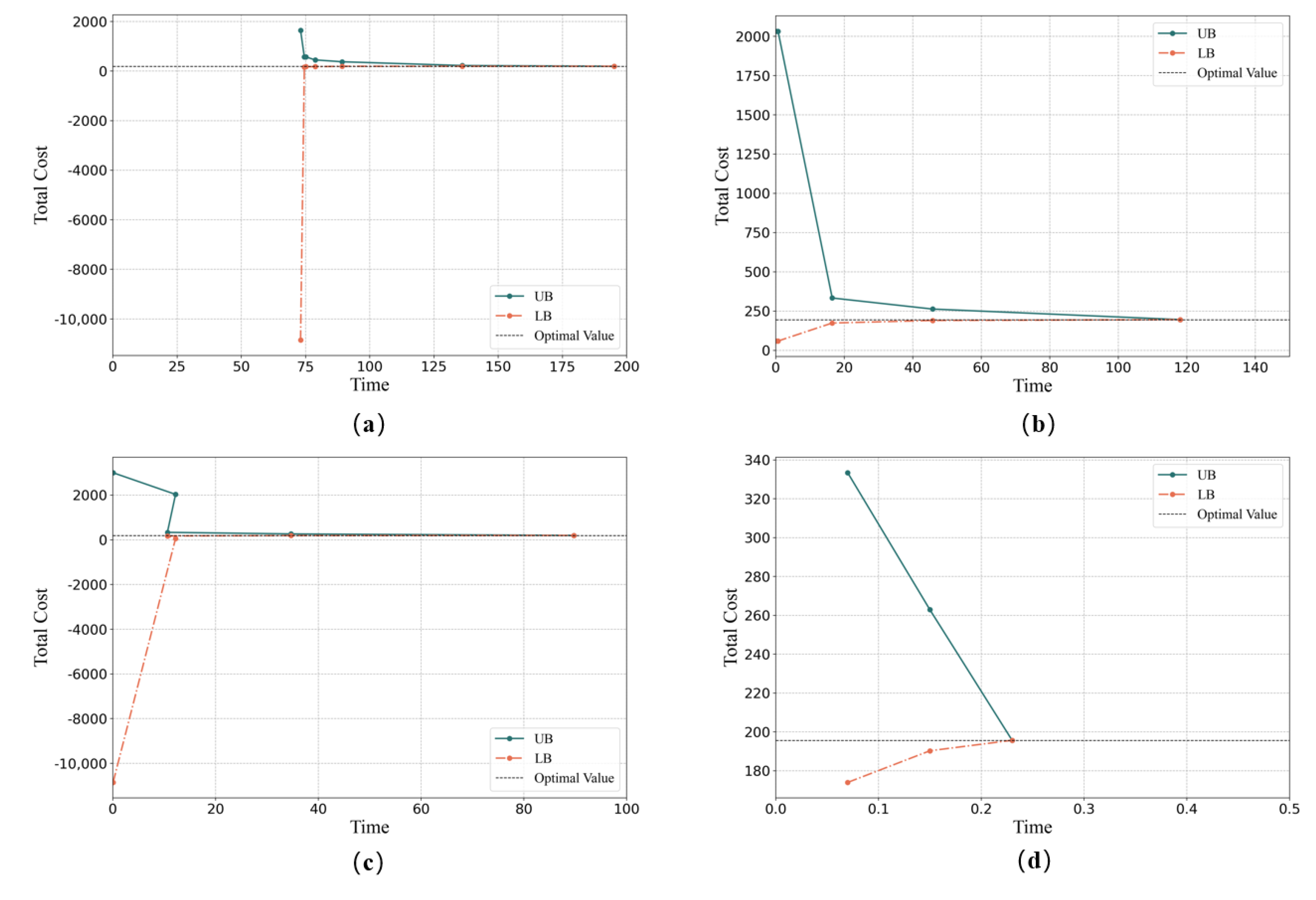
Figure 1 presents the convergence graphs of the four methods solving an instance of 3–10–5–(10,30).
Based on the experimental results above, we can easily have the observations that all of four methods can solve the smallest instances optimally. However, when the problem scale grows, none of them except for the improved C&CG method can optimally solve all instances with a much shorter time. Furthermore, less iterations are taken by the improved C&CG method, which confirms the effectiveness of the heuristic initial solution.
As the scale of the problem continues to grow, it takes more than 1 h for the first three methods to solve the problems. Additionally, there remains big gaps, while the improved C&CG method can solve the instances in a much shorter time. Although the problems might not be optimally solved, only very small average gaps remain.
We notice that, for large instances, the improved C&CG method takes more iterations. This is because the sub-problems of the other three methods are really difficult to solve, most of which take more than 1 h to optimally solve the solver. This proves that the Proposition 2 is extremely effective for our problem.
4.2. Sensitivity Experiments
It should be noticed that the parameter actually plays as a role indicating the maximum number of orders that might deviate from the nominal demands with Proposition 1. When , this means that all of the orders are allowed to deviate from the nominal demands. Furthermore, when , none of the orders can change, and as a result, the 2-RLCBP degenerates into the deterministic one.
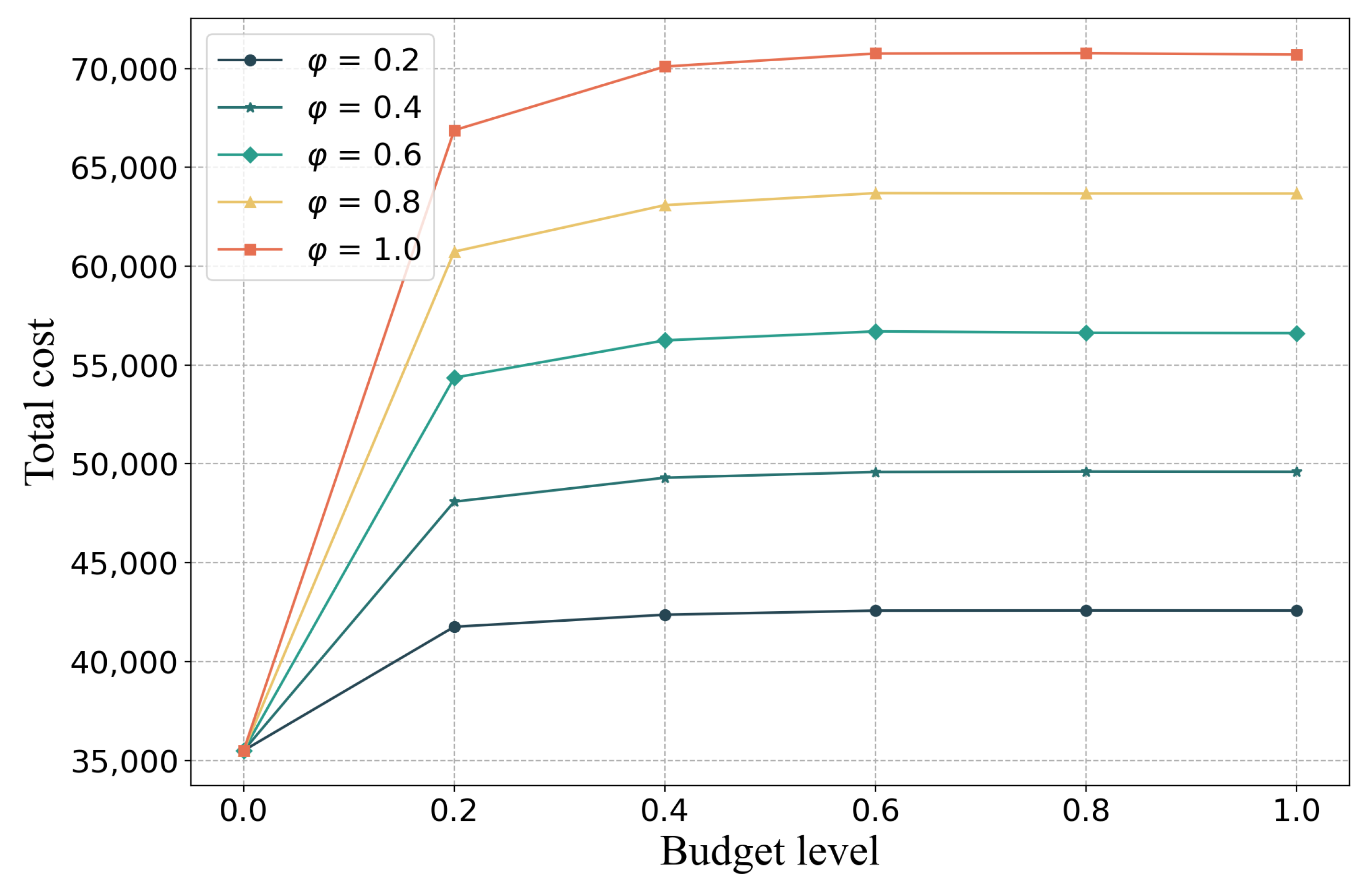
In order to figure out the impact of
on the total cost, a concept budget level is introduced here, whose value equals to
. As can be seen in
Figure 2, under the same value of
, when the budget level is less than 0.2, it has a strong impact on the worst-case total cost. However, as the budget level continues to grow, the impact becomes very slight.
Additionally, under the same budget level, the total cost is also positively correlated with .
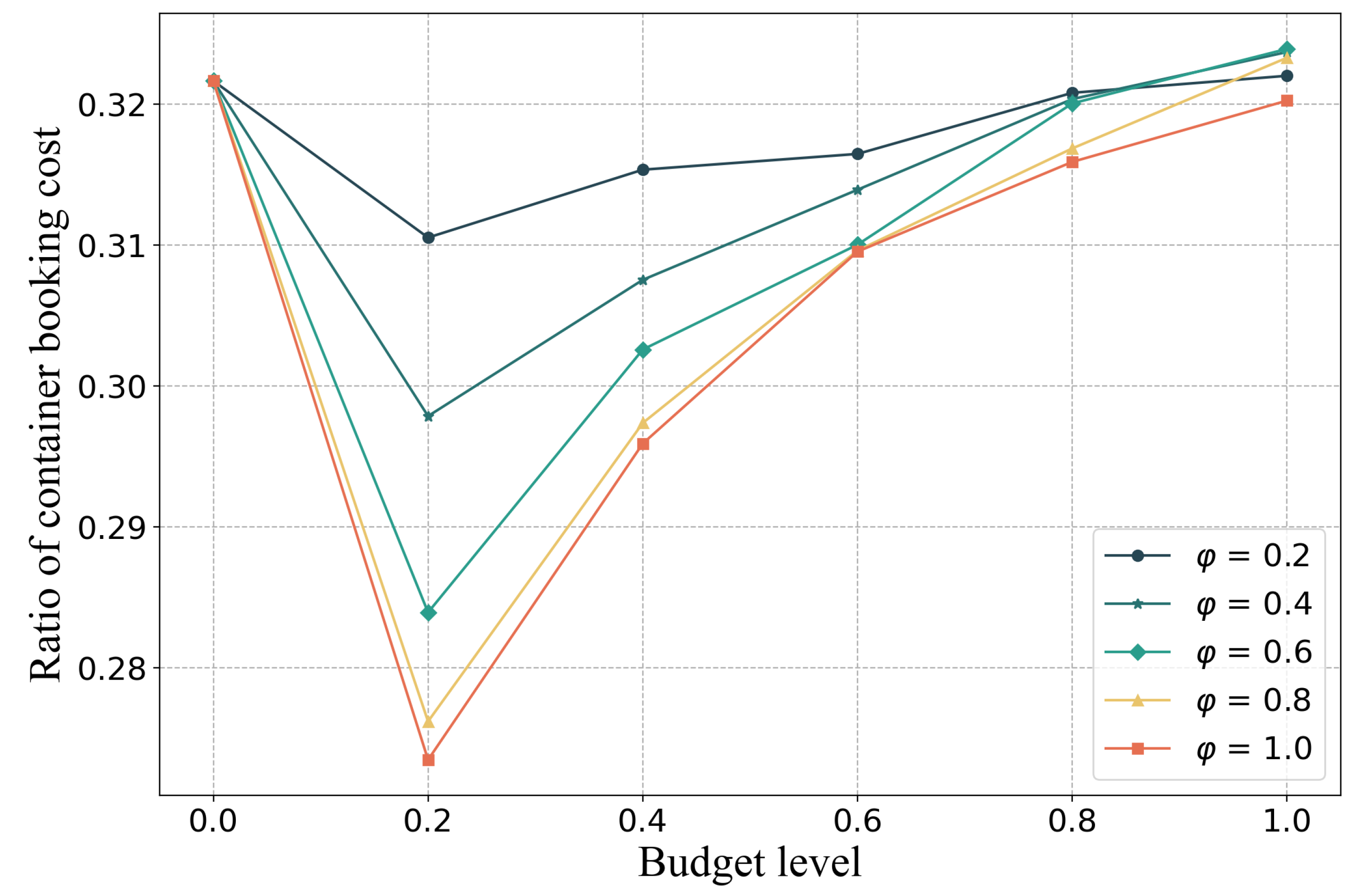
We further explore the impact of the budget level on the proportion of the container booking cost on the total cost. In
Figure 3, as the budget level grows, the proportion of the container booking cost on the total cost drops firstly and reaches its lowest when the budget level meets 0.2. When the budget level is greater than 0.2, the proportion of the container booking cost begins to rise with the increase in budget level.
Overall, the ratio of container booking cost is lower when the corresponding is larger. However, the intervals between adjacent curves are not uniform. When the adjacent curves are of greater s, the interval becomes smaller.
We made a more detailed comparison of the costs under a different budget level and demand deviation level and the results are shown in
Table 4. Set the first row of each demand deviation level as a benchmark, divide the cost of each subsequent rows by the benchmark to obtain the ratio of each cost. It can be seen that for the same demand deviation level, when the budget level increases, the total cost ratio increases, as well as the first-stage costs ratio. Furthermore, the total cost ratio reaches the maximum value faster than the first-stage costs ratio. However, the trend of the second-stage cost ratio is different from the previous two, which increases the first and then decreases.
4.3. Reliability Experiments
In this section, we made a more detailed analysis of the demand deviation level and budget level parameters on both the deterministic model and the 2-RLCBP. Furthermore, we aimed to reveal the reliability of the 2-RLCBP by comparing its solution to that of the deterministic model. We firstly solve the deterministic model on orders of nominal demands and obtain the first-stage container booking cost. Then, by fixing the first-stage decision variables, we can further solve the recourse problem of the C&CG model to obtain the second-stage worst-case cost. The total cost of the deterministic model is obtained by adding the above first-stage container booking cost and second-stage worst-case cost, which provides us with a reference for the cost for not considering the demand uncertainty in advance. As for the two-stage robust model, we just solve it and obtain the worst-case total cost, as well as the first-stage cost and second-stage cost.
We fix the budget level as 0.6, and obtained the costs of different demand deviation levels, which are shown in
Table 5. The lower total costs obtained by the two models at different demand deviation levels are marked in bold. As can be seen from the table, the total cost of 2-RLCBP is significantly lower than that of the deterministic model. More specifically, when
, compared to the deterministic model, the 2-RLCBP has higher-first-stage container booking cost, whose second-stage unfulfilled order penalty cost, on the other hand, is much lower. Furthermore, an increasing gap between the costs of the two models shows as the demand deviation level becomes higher.
Table 6 shows the results of the two models with a demand deviation level fixed to 0.6 and the budget level varying in [0,1]. The lower total costs obtained by the two models at different budget levels are marked in bold. Similar observations can be obtained in this table.
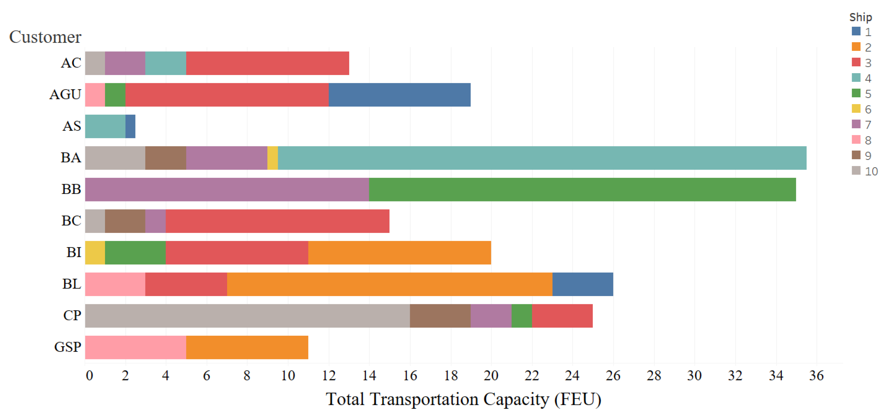
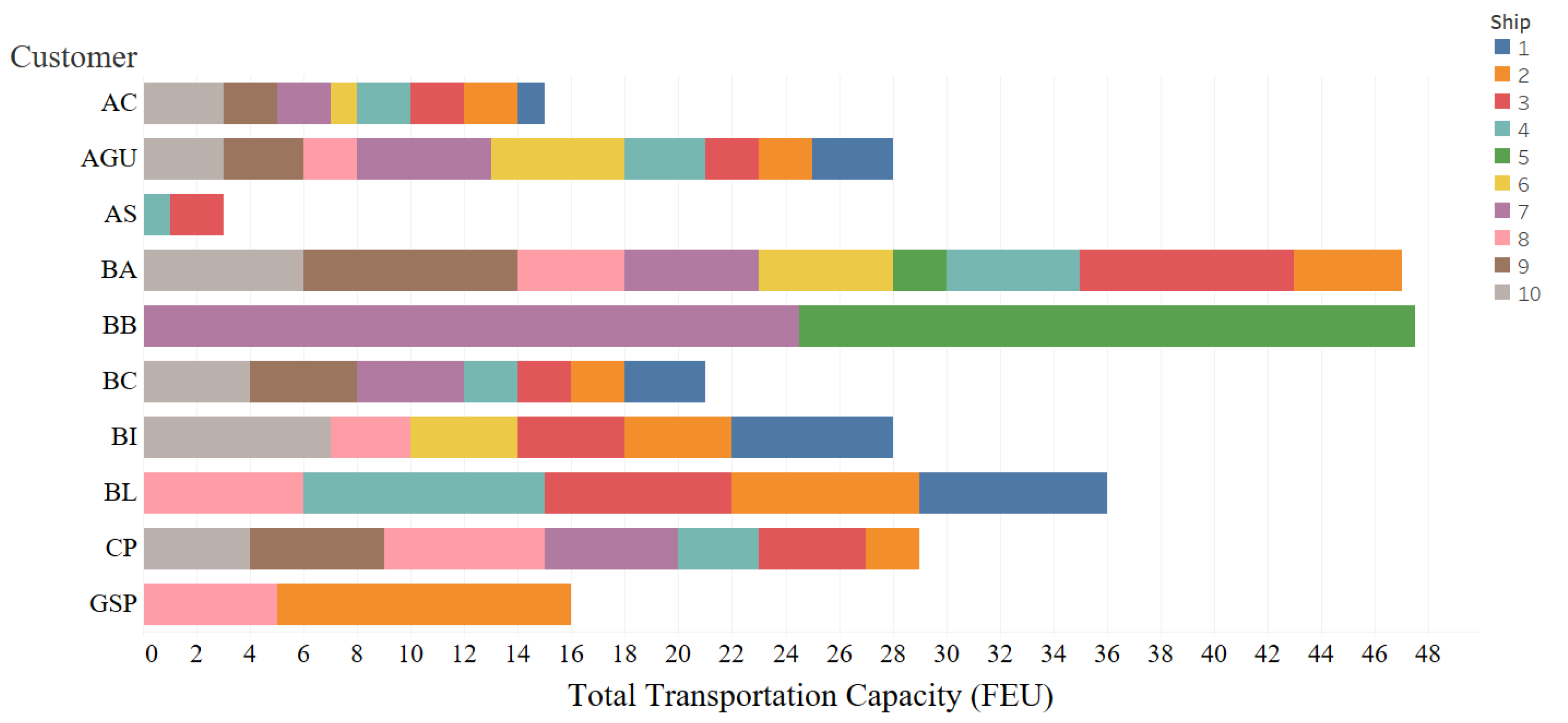
To illustrate the impact of demand uncertainty on the solution structure, we randomly select an instance of 10–20–10–(20,60).
Figure 4 and
Figure 5 show the solutions of the transport capacity booked for each customer, which is obtained by solving the deterministic model and 2-RLCBP, respectively.
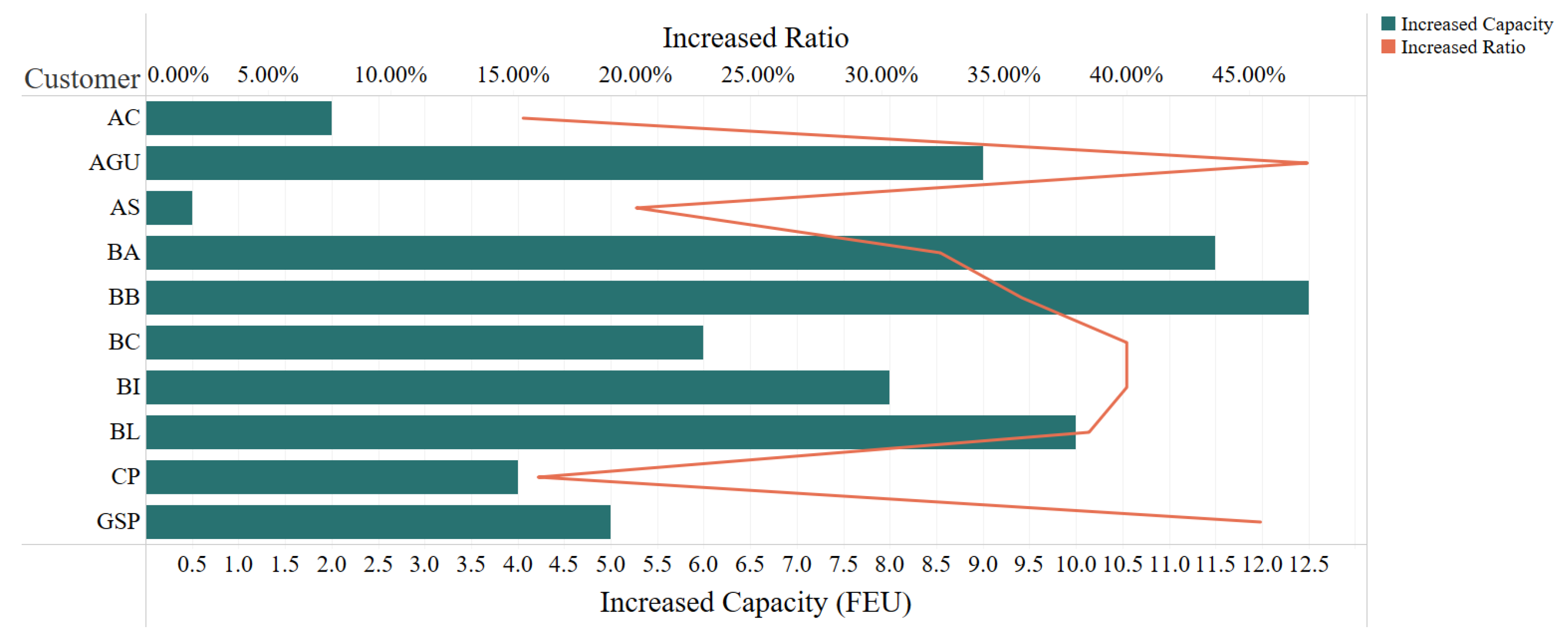
Table 7 shows the transportation capacity booked for each customer in the solution of 2-RLCBP and deterministic model. For a more visual illustration,
Figure 6 is presented.
We can find that the transport capacity booked for each customer in the robust solution is slightly greater than that in the deterministic solution. In addition, customers who need more transport capacity in the deterministic solution would be more likely to obtain a higher increase in transport capacity in the robust solution.
Furthermore, compared to the deterministic model, 2-RLCBP tends to present a situation in which the transportation capacity assigned to each customer is more decentralized. In other words, in the result of the deterministic model, most of the needed transportation capacity of each customer is concentrated in one or two ships, while 2-RLCBP shows that each customer tends to use more ships and the applied transportation capacity is more evenly distributed across more ships.
In real-world application, our methodology can be integrated into the company’s system. When the container booking decision is required, enter the relevant data such as the nominal customer demand, the inventory volume, and the container information into the system, and the optimal booking decision can be obtained for the logistics planning department. Additionally, the logistics planning department can adjust the budget level to take into account the actual situation faced by the company so as to obtain more practical decisions.
5. Discussion
In the present study, we propose a two-stage robust approach to deal with the liner container booking problem with uncertain customer demand. We guarantee the results through rigorous mathematical derivation in the proposed methodology. Furthermore, to further verify the results, we conducted a series of experiments based on both random instances and real-case instances.
The computational performance experiments shows that the proposed C&CG algorithm is of high efficiency compared to other methods. There are two main reasons for this. Firstly, the proposed heuristic initial solution-generating algorithm can offer a good initial solution, which can reduce the iteration of the C&CG algorithm. Secondly, and more importantly, the proposed upper bounds of the variables of the dual sub-problem can significantly narrow the domain when solving the dual sub-problem.
In the sensitivity experiments, we found that there is a sharp increase in the total cost when the budget level increases from 0 to 0.2. After that, the curve of the total cost becomes very smooth. This is because, in the worst cases, the orders with greater demands are more likely to deviate from the nominal demands, which can also be found in the final solutions. Furthermore, it can be found in the data that a small percentage of orders account for a large part of the total demand. Thus, when the budget level is low, the big orders tend to deviate from nominal demands, have high influence, which leads to the sharp increase in the total cost. As the budget level continues to grow, demands for smaller orders begin to fluctuate, however, the influence of this is much smaller. Similarly to the above explanation, the reason for the appearance of such a V-shaped curve in
Figure 3 is that, when the budget level is small, the orders with greater demands are more likely to deviate from the nominal demands which lead to a higher penalty for unfulfilled orders. Thus, compared to the increase in the penalty, the ratio of the container booking cost becomes lower. As the budget level continues to grow, small orders begin to deviate from the nominal demands, which, however, would not be highly penalized. However, on the other hand, more containers are still needed to face future uncertainty, which leads to the rise in the ratio of the container booking cost. Thus, paying attention to the demand fluctuation of the orders with relatively large requirements is quite important for companies when making the container booking decision, which also proved the effectiveness of our heuristic initial solution generation method. Additionally, it is not economically worthwhile to consider the solution under a high budget level for companies.
In the reliability experiments, it can clearly be seen that the total cost obtained by the two-stage robust optimization model is much lower compared to that given by the deterministic model. Furthermore, the gap between the total costs obtained by the two models grows as the demand deviation level and budget level grow. This is because the deterministic model completely ignores the customer demand uncertainty, which leads to the rapid increase in the second-stage cost of the deterministic model when the uncertainty intensifies. Therefore, the robustness of the proposed two-stage robust optimization approach has been well verified.
The experimental results verify the effectiveness of the proposed two-stage robust optimization approach in dealing with the customer demand uncertainty, which also provides a reference for the companies on how to make container booking decisions.
6. Conclusions
The present study investigates a liner container booking and freight consolidation problem, which takes the customer demands uncertainty into account. A two-stage robust optimization model is presented and the decisions are made in two stages. In the first stage, containers of different types are booked for each customer without the actual information of the customer demand. Furthermore, in the second stage, the order fulfillment plans, i.e., the freight consolidation and containerization decisions, are made with the revealed customer demand information. Furthermore, the uncertainty of customer demand is characterized with a budgeted uncertainty set. Given the specific feature of the tire transportation problem, by relaxing the container capacity constraints, a more streamlined model is obtained. Then, we develop a C&CG algorithm to solve the problem. To enhance the efficiency of the algorithm, a heuristic is developed to generate initial solutions, which can help reduce the number of iterations of the algorithm.
In the methodological approach, we conducted rigorous mathematical derivation, and the bi-level sub-problem is reformulated into an equivalent mixed-integer linear programming model that can be solved by the off-the-shelf solver by applying the duality theory. By analyzing the problem structure, a tight upper bound of the three dual variables can be obtained, which can greatly reduce the computation time of the dual sub-problem. We also adapt the Benders-dual method to solve the problem as a comparison. The numerical experiment results show the high efficiency of the proposed C&CG algorithm. Furthermore, the sensitivity analysis is conducted based on the real data to determine the impact of the budget level on the total cost and the ratio of the container booking cost. Furthermore, it is observed that a low budget level would have a greater impact on the results. For companies, it is not economically worthwhile to consider the solution under a high budget level. In the reliability analysis, we compare the results of 2-RLCBP to those of the deterministic model. Furthermore, the results show that 2-RLCBP can secure a lower total cost under different demand deviation levels and budget levels, which verifies the outstanding worst-case performance of the proposed two-stage robust optimization approach.
Our work adopts the perspective of a manufacturing company, talking about the container booking problem faced by the manufacturing companies considering the uncertain customer demand. Furthermore, we are the first to propose the two-stage robust optimization approach for this problem. In this paper, we only consider the uncertainty of the customer demand. However, in real life, uncertainty can appear in various aspects. One interesting future research direction is to consider more uncertainty at the same time. For example, the available transportation capacity provided by 3PL could also be uncertain influenced by various factors such as uncontrollable markets or disasters. By considering more uncertain factors, more practical decisions can be provided to the companies, which is important to reduce the logistics costs.


