Image Hiding in Stochastic Geometric Moiré Gratings

Abstract

An image hiding scheme based on stochastic moiré gratings is proposed, discussed, and illustrated in this paper. The proposed scheme is based on a counter-intuitive optical feature of specially designed stochastic moiré gratings when similar images in the static mode become very different in the time-averaged mode. A soft computing PSO algorithm was used for the construction of stochastic gratings. Complex computational algorithms were required to construct the cover image; however, the decryption process was completely visual. The cover image must oscillate in a predefined direction and at a predefined amplitude (the amplitude of the harmonic oscillation is one of the parameters of the proposed image hiding scheme). Computational experiments were used to demonstrate the efficacy of this optical image hiding scheme based on the stochastic moiré gratings.

1. Introduction

Geometric moiré is a classical optical experimental technique used for the experimental identification of displacements, strains, etc., from the patterns of moiré fringes [1,2,3,4]. Geometric moiré is classified into double exposure geometric moiré and time-averaged geometric moiré [1,2]. Both optical techniques require the formation of moiré gratings on the surface of a deformable object. Double exposure geometric moiré uses the superposition of two images. The first image of the moiré grating is taken in the state of equilibrium. The second image of the grating is taken in a deformed state. Two static moiré gratings yield a two-dimensional pattern of fringes used to describe the spatial field of in-plane deformations.

Time-averaged geometric moiré techniques use exposure times such that many oscillation periods fit into the averaging interval. Naturally, time-averaged geometric moiré techniques are commonly used for vibrating deformable bodies [2].

Two main goals exist in the analysis of moiré patterns (generated by double exposure or time-averaged techniques). The first goal deals with the interpretation of experimentally obtained patterns of moiré fringes. Those patterns are used to reconstruct the field of displacements, strains, etc., at the centerlines of moiré fringes [2,3,4]. The other goal is associated with the synthesis of a predefined target pattern of moiré fringes [5,6]. Note that there is a tight link between both tasks as one task gives insight into the other.

Recently, moiré techniques have been successfully exploited in different image hiding applications. For example, an image encryption technique based on embedding the secret image into the geometric moiré pattern is discussed in [7]. Unfortunately, with this method, rough details of the secret image may still be visible in the deformed pattern of moiré grating lines, even to the naked eye. To address this issue, an improved algorithm for image encryption and decryption that uses stochastic moiré grating manipulations is presented in [8]. In this approach, the secret information is hidden by deforming a stochastic moiré grating according to the grayscale intensities of the secret image. Decryption is performed by correlating the pixel intensities in the encrypted image and the original stochastic moiré grating [8].

The relationship between the pitch of the moiré grating, the order of the time-averaged fringe, and the amplitude of the harmonic oscillations forms the basis for the dynamic visual cryptography (DVC) image hiding technique [9]. This term (DVC) originates from the concept of visual cryptography (VC), which was introduced in 1995 [10]. VC can be characterized by two basic features. Complex computational algorithms are required to encode the secret image. However, a computer is not required to decode the image; the secret is revealed and can be interpreted by the naked eye [10]. VC algorithms are used to split the secret image into two (or more) separate shares (usually printed on transparencies). The secret image emerges when those transparencies are aligned and stacked together [10].

DVC is not based on image sharing [9]. The secret dichotomous image is embedded into the moiré grating in such a way that the stationary cover image does not reveal any hidden information, but the secret can be decoded as a pattern of time-averaged moiré fringes when the cover image oscillates harmonically with a predefined amplitude a, and time-averaging techniques are used to register the time-averaged image [9]. The secret can be directly visually decoded by observing the oscillating cover image. The naked human eye is capable of integrating oscillating images over time and perceiving embedded secret information only if the minimum frequency of oscillations exceeds 25–28 Hz [11].

The main objective of this paper is to introduce stochastic moiré gratings into DVC schemes, which enables an increase in the security of the cover image. The main advantage of the proposed DVC scheme is based on the fact that the stochastic structure of the cover image ensures robustness to statistical algorithms. In other words, statistical analysis of the stationary cover image cannot reveal the encoded visual information.

This paper is structured as follows. Section 2 discusses the one-dimensional Wada index, governing equations of time-averaged geometric moiré, and the scheme for image hiding in harmonic gratings. The construction of the dynamic visual cryptography scheme based on near-optimal stochastic gratings is introduced in Section 3. Concluding remarks are presented in the last section.

2. Preliminaries

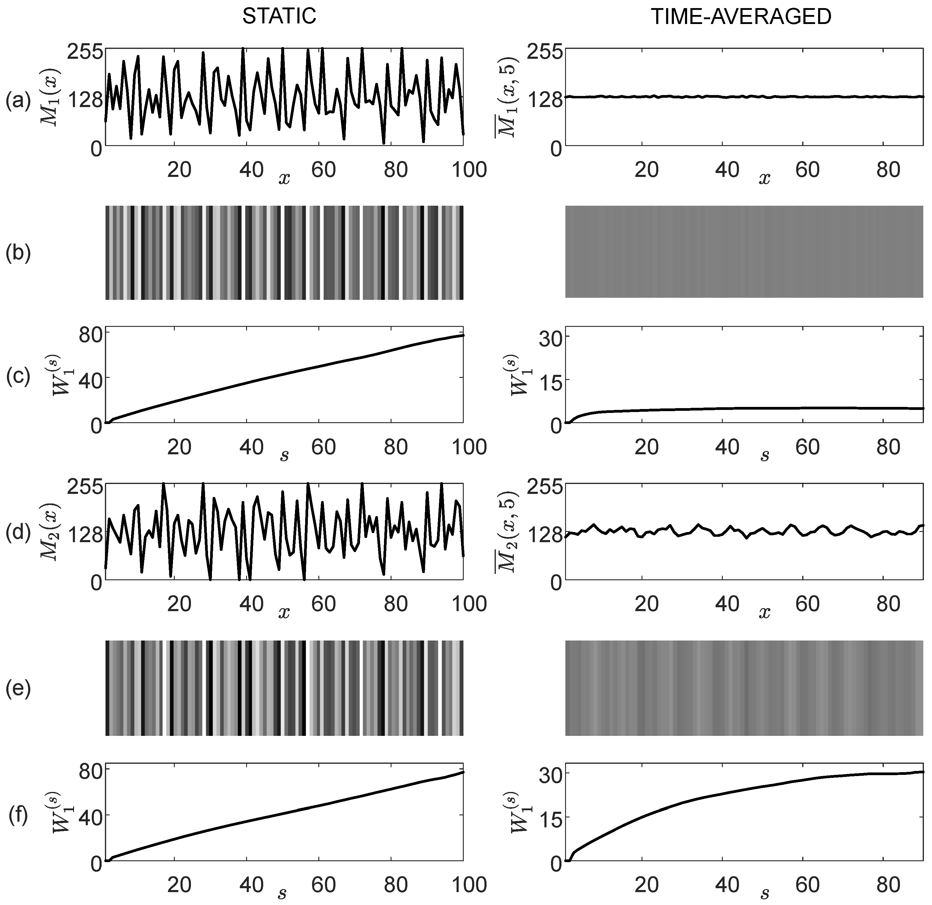
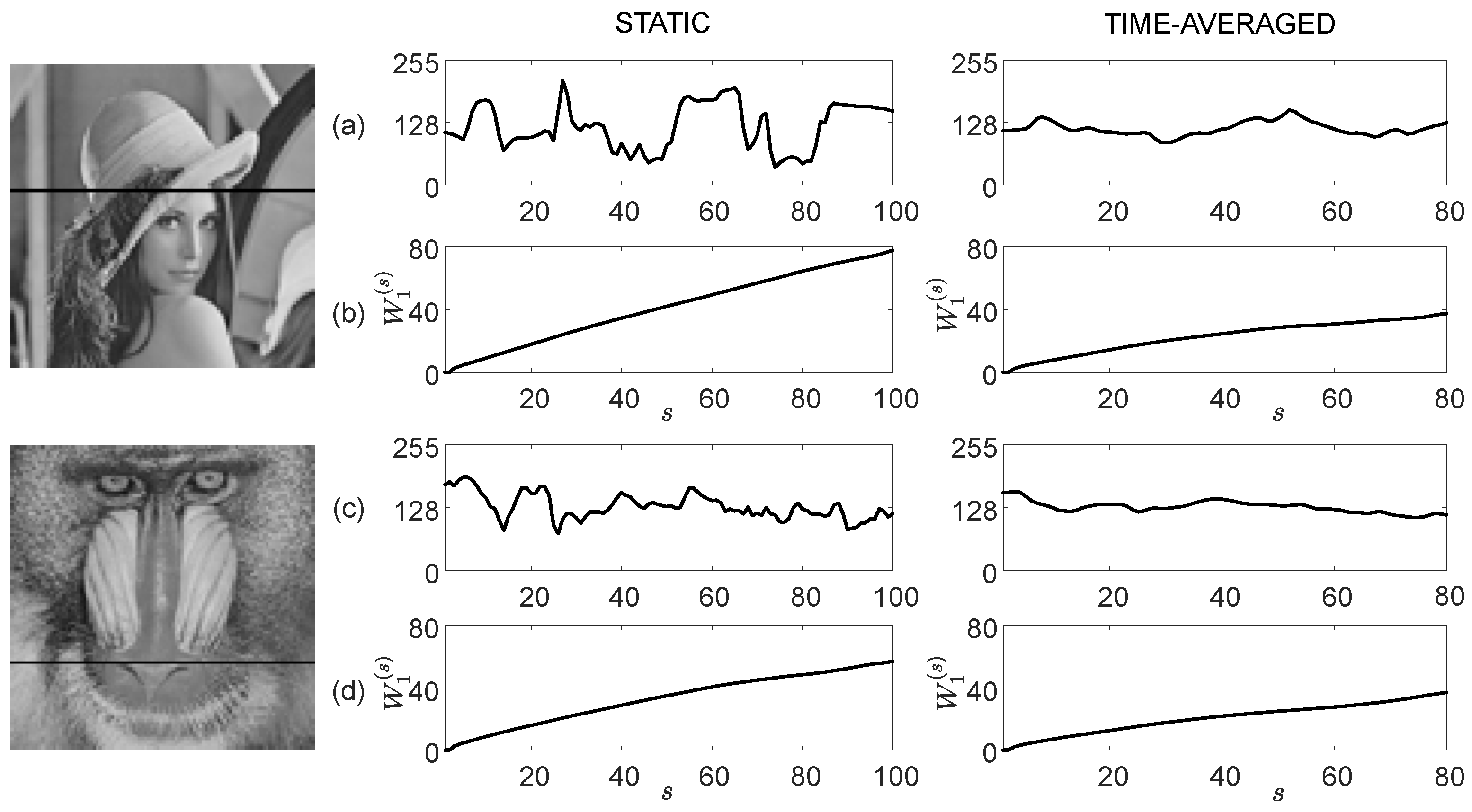
2.1. The Wada Index for the Evaluation of the Grating Complexity

It is common to evaluate the randomness of digital grayscale images using the Shannon entropy [12,13]. In [14], the Wada index, based on weighted and truncated Shannon entropy, was proposed for detecting Wada boundaries in phase plots of nonlinear dynamical systems. Moreover, the Wada index provides a numerical estimate of the number of different colors and their proportions in a two-dimensional phase space diagram, making it applicable not only in nonlinear dynamics but also in image processing in general [14]. In this study, the Wada index is used to estimate the number of different grayscale levels and their distribution in stationary and time-averaged moiré gratings.

Let us list the notations required for the introduction of the one-dimensional (1D) Wada index, which is used to evaluate the complexity of the 1D digital image:

• s—The length of the 1D observation window measured in the number of pixels; $s\ge 2$.
• c—The number of different grayscale levels in the 1D observation window; $c\ge 1$.
• ${\nu }_k$, $k=1,2,\dots ,c$—The number of k-th color pixels in the 1D observation window.
• $p_k=\frac{{\nu }_k}{s^2}$, $k=1,2,\dots ,c$—The discrete probability of the k-th color in the 1D observation window.
• The indicator function ${\mathbf{1}}_2^{\left(s\right)}$ is equal to 1 if the number of grayscale levels in the 1D observation window is greater than or equal to 2: ${\mathbf{1}}_2^{\left(s\right)}=\left\{\begin{array}{c}1,c\ge 2,\\ 0,c=1.\end{array}\right.$
• The indicator function ${\mathbf{1}}_3^{\left(s\right)}$ is equal to 1 if the number of grayscale levels in the 1D observation window is greater than or equal to 3: ${\mathbf{1}}_3^{\left(s\right)}=\left\{\begin{array}{c}1,c\ge 3,\\ 0,c\le 2.\end{array}\right.$
• The Shannon entropy of different grayscale levels in the 1D observation window:

  $$e^{\left(s\right)}\left(p_1,p_2,\dots ,p_c\right)=-\sum _{k=1}^c{p}_{k}log\left(p_k\right).$$

  (1)

The Wada index ${\omega }_1^{\left(s\right)}$ in the 1D observation window of length s reads [14]:

$$\begin{array}{c}\hfill {\omega }_1^{\left(s\right)}\left(p_1,p_2,\dots ,p_c\right)=\frac{c}{log\left(c\right)}{\mathbf{1}}_3^{\left(s\right)}{e}^{\left(s\right)}=\left\{\begin{array}{c}0,c<3,\hfill \\ -\frac{c}{log\left(c\right)}\sum _{k=1}^c{p}_{k}log\left(p_k\right),c\ge 3.\hfill \end{array}\right.\end{array}$$

(2)

Let us denote the number of 1D observation windows covering the whole 1D digital image as N. Then, the Wada index $W_1^{\left(s\right)}$ for the whole 1D digital image can be formulated in accordance with [14]:

$$W_1^{\left(s\right)}=\frac{{\sum }_{k=1}^N{\omega }_{1,k}^{\left(s\right)}}{{\sum }_{k=1}^N{\mathbf{1}}_{2,k}^{\left(s\right)}},$$

(3)

where ${\omega }_{1,k}^{\left(s\right)}$ and ${\mathbf{1}}_{2,k}^{\left(s\right)}$ are the Wada index ${\omega }_1^{\left(s\right)}$ (Equation (2)) and the indicator function ${\mathbf{1}}_2^{\left(s\right)}$ in the k-th observation window.

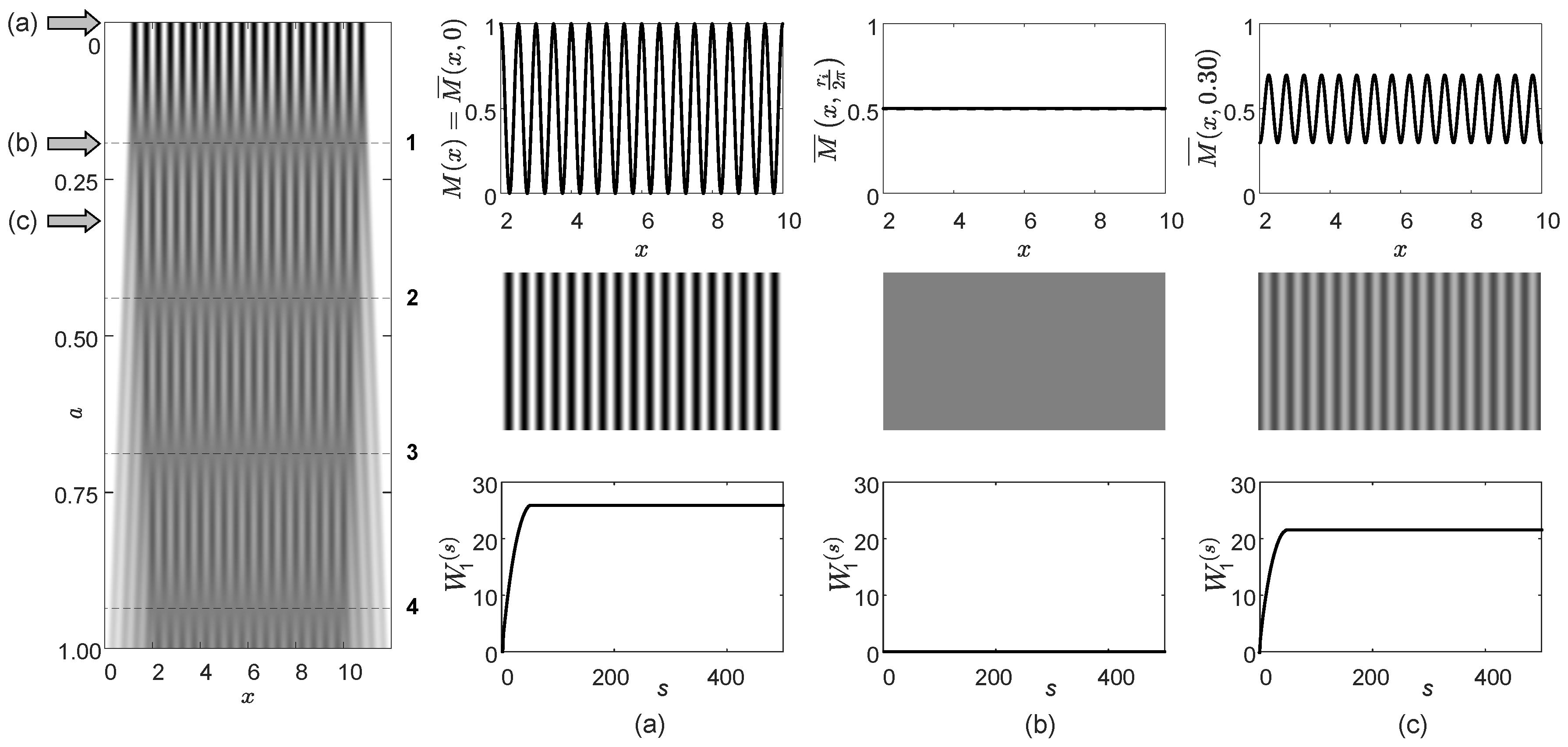
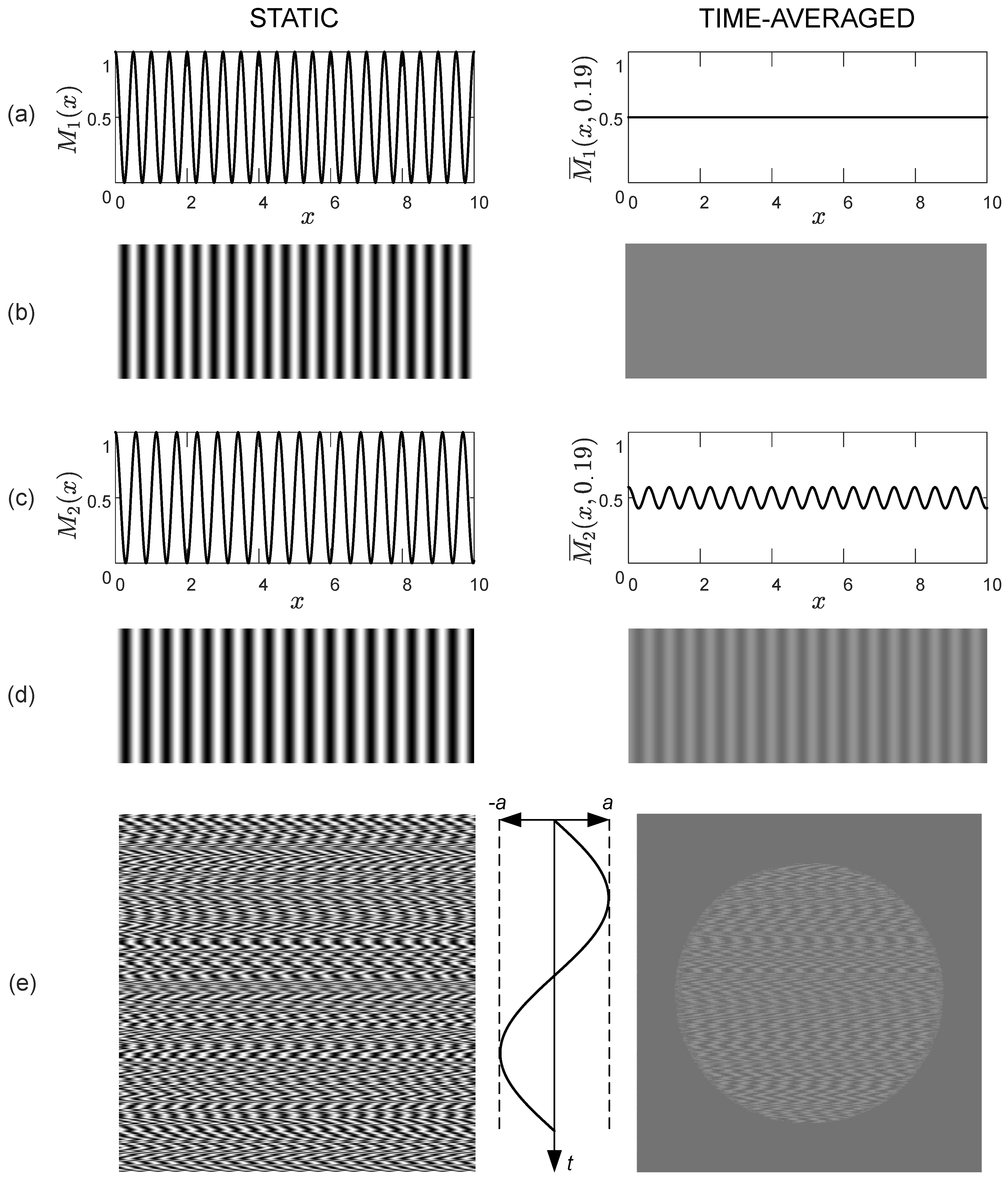
2.2. Time-Averaged Geometric Moiré: Harmonic Grating

The one-dimensional harmonic moiré grating $M\left(x\right)$ in the state of equilibrium reads:

$$M\left(x\right)=\frac{1}{2}+\frac{1}{2}cos\left(\frac{2\pi }{\lambda }x\right),$$

(4)

where x is the one-dimensional spatial coordinate; $\lambda$ is the pitch of the grating, indicating the distance between the centers of two adjacent white (or black) grating lines. Values of $M\left(x\right)$ vary from 0 (which corresponds to the black color) to 1 (the white color); values from the interval $[0,1]$ represent different grayscale levels.

Let us suppose that the moiré grating $M\left(x\right)$ (Equation (4)) oscillates in time according to the harmonic function $asin\left(\omega t+\phi \right)$ in the direction perpendicular to the grating lines (a, $\omega$ and $\phi$ stand for the amplitude, frequency, and phase of harmonic oscillations, respectively). The brightness of the gray color at point x at time moment $t_0$ reads:

$${\left.M\left(x\right)\right|}_{t=t_0}=\frac{1}{2}+\frac{1}{2}cos\left(\frac{2\pi }{\lambda }\left(x-asin\left(\omega t_0+\phi \right)\right)\right).$$

(5)

If time-averaging techniques are used to register the image in Equation (5) for a sufficiently long exposure time T, the grayscale time-averaged image reads [2]:

$$\begin{array}{c}\hfill \overline{M}\left(x,a\right)=\underset{T\to \infty }{lim}\frac{1}{T}{\int }_0^{T}M\left(x-asin(\omega t+\phi )\right)dt=\frac{1}{2}+\frac{1}{2}cos\left(\frac{2\pi }{\lambda }x\right)J_0\left(\frac{2\pi }{\lambda }a\right),\end{array}$$

(6)

where $J_0$ is the zero-order Bessel function of the first kind:

$$J_0\left(x\right)=\underset{T\to \infty }{lim}\frac{1}{T}{\int }_0^{T}exp\left(i·xsin\left(\omega t+\phi \right)\right)dt;i^2=-1.$$

(7)

It is clear that the brightness of the grayscale color in the time-averaged geometric moiré depends only on the amplitude of the harmonic oscillations. The oscillation frequency $\omega$ and the phase $\phi$ have no influence on the time-averaged $\overline{M}\left(x,a\right)$ (when $T\to \infty$).

The computational representation of $\overline{M}\left(x,a\right)$ (Equation (6)) can be implemented by computing the arithmetic average of ${\left.M\left(x\right)\right|}_{t=t_k}$ ($k=1,2,3,\dots$) over one period of harmonic oscillations ($0\le t_k<2\pi$) [9]:

$$\begin{array}{c}\hfill \overline{M}\left(x,a\right)=\underset{n\to \infty }{lim}\frac{1}{n}\sum _{k=1}^n{\left.M\left(x\right)\right|}_{t=t_k}\approx \frac{1}{n}\sum _{k=1}^n{cos}^2\left(\frac{\pi }{\lambda }\left(x-asin\left(\frac{2\pi }{n}(k-1)\right)\right)\right).\end{array}$$

(8)

The accuracy of a numerical reconstruction of the time-averaged image is determined by the number of discrete time steps n used in one period of oscillations (Equation (8)). The relationship between n and the number of reconstructed time-averaged moiré fringes with a predefined accuracy is given in [9].

Time-averaged moiré fringes become fully developed when

$$J_0\left(\frac{2\pi }{\lambda }a\right)=0.$$

(9)

The relationship between the sequential number of time-averaged fringes, the amplitude of harmonic oscillations, and the pitch of the moiré grating reads:

$$\frac{2\pi }{\lambda }{a}_i=r_i,$$

(10)

where $r_i$ denotes the i-th root of $J_0$ (Equation (7)); $a_i$ is the amplitude of oscillations at the center of the i-th time-averaged fringe.

The graphical interpretation of Equation (10) is presented in Figure 1. One-dimensional time-averaged moiré gratings $\overline{M}\left(x,a\right)$ at increasing amplitudes of harmonic oscillations a are depicted in the left panel of Figure 1. Note that the top row of this image (at $a=0$) coincides with the stationary moiré grating $M\left(x\right)$. The stationary moiré grating $M\left(x\right)$, its optical representation, and the Wada index $W_1^{\left(s\right)}$ are depicted in Figure 1a. Note that $0\le M\left(x\right)\le 1$, but the brightness of pixels in the optical representation varies from 0 to 255.

The panels representing Wada indexes in Figure 1 are constructed in such a way that the horizontal axis represents the length of the 1D observation window s. In other words, Figure 1 represents the variation of the Wada index $W_1^{\left(s\right)}$ in respect to s. The Wada index $W_1^{\left(s\right)}$ is depicted at $a=0$ (Figure 1a), the middle of the first time-averaged moiré fringe ($a=\frac{\lambda r_1}{2\pi }\approx 0.1914$, Figure 1b), and the zone between the first and the second time-averaged fringes ($a=0.3$, Figure 1c).

Note that $W_1^{\left(s\right)}$ is a monotonous function with respect to s. The wider the observation window, the larger the number of pixels with different brightness. The maximum value of $W_1^{\left(s\right)}$ is produced at the largest s. However, periodic moiré gratings (Figure 1a,c) yield maximum values of $W_1^{\left(s\right)}$ even when the width of the observation window is equal to one period of the grating.

Time-averaged moiré gratings become continuously gray (the time-averaged fringes becomes fully developed) at $a=\frac{\lambda r_i}{2\pi },i=1,2,3,\dots$ (see Equation (10) and Figure 1b). The time-averaged moiré fringe is not fully developed when amplitude a does not satisfy Equation (10). This fact is illustrated in Figure 1c.

2.3. Image Hiding in Harmonic Gratings

Let us suppose that two moiré gratings $M_1\left(x\right)$ and $M_2\left(x\right)$ are given with two different pitches ${\lambda }_1=0.5$ and ${\lambda }_2=0.57$. Static moiré gratings $M_1\left(x\right)$ and $M_2\left(x\right)$ are depicted in Figure 2a,c. Optical representations of the static moiré gratings $M_1\left(x\right)$ and $M_2\left(x\right)$ are depicted in Figure 2b,d.

Both moiré gratings are oscillated harmonically with the same amplitude of oscillations $a=0.19$ (Figure 2). Time-averaged moiré gratings ${\overline{M}}_1\left(x,0.19\right)$ and ${\overline{M}}_2\left(x,0.19\right)$ are shown in Figure 2a,c; their optical representations are shown in Figure 2b,d.

The amplitude of harmonic oscillations $a=0.19$ is preselected in such a way that the pitch ${\lambda }_1=0.5$ satisfies Equation (10). The time-averaged image ${\overline{M}}_1\left(x,0.19\right)$ becomes plain gray and the time-averaged fringe becomes fully developed (Figure 2b).

However, amplitude $a=0.19$ and the pitch ${\lambda }_2=0.57$ do not satisfy the relationship given by Equation (10). The time-averaged moiré fringe is not fully developed, and the blurred original moiré grating is still visible in the resulting time-averaged image (Figure 2d).

The DVC encoding scheme is illustrated by a simple computational example when a plain circle is embedded into the surrounding background (Figure 2e). The stochastic initial moiré phase algorithm and the algorithm for the regularization of moiré phases on the boundary lines between the secret and the background [9] are used to hide the “secret” circle in the background (Figure 2e). The naked eye cannot interpret the secret image in the stationary encoded image.

However, the secret image is leaked when the amplitude of harmonic oscillations is preselected in such a way that a fully developed moiré fringe is formed either in the background or in the area occupied by the secret image. The Moiré grating $M_1\left(x\right)$ is used to cover the background; the moiré grating $M_2\left(x\right)$ is the area occupied by the circle. Therefore, the background becomes plain gray, and the circle appears in the form of not-fully developed moiré fringe in the time-averaged image in Figure 2e.

The image hiding scheme in harmonic gratings (the DVC scheme based on harmonic moiré gratings) can be characterized by the two essential features. The secret image should be unrecognizable to the naked eye from the stationary cover image. The secret image should be interpretable to the naked eye when the cover image oscillates, and the amplitude of harmonic oscillations is set to a given value (the amplitude of harmonic oscillations is one of the keys used for decoding the secret) [9].

2.4. Time-Averaged Random Moiré Grating

Two moiré gratings ($M_1\left(x\right)$ and $M_2\left(x\right)$) used to construct the DVC scheme in Figure 2 are harmonic functions. Moreover, although the naked eye cannot interpret the embedded secret in the static cover image, advanced statistical algorithms could be exploited to check the variations in the period of the pixel brightness in each row of the digital cover image.

The robustness of the DVC scheme to statistical algorithms can be enhanced by using non-harmonic oscillations [15], near-optimal periodic gratings [16], chaotic oscillations [17], and deformable periodic gratings [18].

Nevertheless, the periodicity of the moiré grating in DVC schemes is a drawback from the point of view of the robustness of steganalysis algorithms. Note that VC schemes are completely robust to steganalysis [10,19]. However, VC schemes are required to split the secret image into shares. The fact that the secret image is split into separate shares also raises serious security issues. VC schemes suffer from the possibility of cheating when the eavesdropper obtains information about one of the shares and can generate another/other share/shares in order to produce fake secret images [19]. Special advancements in VC schemes help to lower the cheating probability, but it remains an issue related to the security of those schemes [20,21].

Therefore, the ability to exploit random non-periodic moiré gratings in DVC schemes remains an attractive objective, which could raise the security of those schemes to another level.

Time-averaged patterns produced by random moiré gratings are discussed in [22]. Time-averaging effects produced by random moiré gratings are illustrated in Figure 3. One-dimensional time-averaged random moiré gratings $\overline{M}\left(x,a\right)$ at increasing amplitudes of harmonic oscillations a are depicted in the left panel of Figure 3. Note that the top row of this image (at $a=0$) coincides with the stationary random moiré grating $M\left(x\right)$. The stationary random moiré grating $M\left(x\right)$, its optical representation, and the Wada index $W_1^{\left(s\right)}$ are depicted in Figure 3a.

The time-averaged random moiré grating $\overline{M}\left(x,a\right)$ at $a=0.4$, its optical representation, and the Wada index $W_1^{\left(s\right)}$ are depicted in Figure 3b. The higher the value of the amplitude of harmonic oscillations, the larger the motion-induced optical blur, and the lower the maximum value of the Wada index $W_1^{\left(s\right)}$ in the time-averaged image (Figure 3b,c).

3. Dynamic Visual Cryptography Based on Stochastic Gratings

3.1. One-Dimensional Stochastic Gratings for Image Hiding Applications

As mentioned previously, all available DVC schemes exploit the relationship between the pitch of the periodic moiré grating, the parameters of oscillations, and the order of the time-averaged fringe to hide the secret in a single cover image. Such DVC schemes are based on the phase regularization and random initial phase shifting algorithms [9]. The secret information is leaked as a pattern of time-averaged moiré fringes when the cover image oscillates at a predefined amplitude, and time-averaging techniques (or the naked eye) are used to register the time-averaged image [11].

The main objective of this paper is to introduce stochastic moiré gratings into DVC schemes. The apparent simplicity of the problem is truly misleading. The stationary cover image must remain uninterpretable (the secret image should not be directly leaked from the stationary image). The secret image should be leaked in the time-averaged image when the cover image oscillates according to a pre-set amplitude of harmonic oscillations. Clearly, phase regularization and random initial phase shifting algorithms are not applicable for stochastic moiré gratings (the concept of the phase is lost in the set of pixels with random brightness). Moreover, changes in the contrast of stochastic images affected by motion blur are completely different from the mathematical point of view. As discussed in the previous section, DVC schemes with harmonic gratings are based on Bessel functions and the interplay of their roots. A completely new nomenclature has to be introduced in order to describe (and control) motion-induced blur for stochastic gratings.

Recently, the Wada index was introduced to measure the randomness of digital images that are more complex than fractal dichotomous basin boundaries of nonlinear dynamical systems [14]. Since the stochastic DVC scheme is based on manipulation with pixels in separate rows (columns) of the cover image, the concept of the Wada index needs to be adapted to one-dimensional sets of pixels (Section 2.1).

The proposed DVC scheme based on stochastic moiré gratings is also based on the interplay between two gratings, where one grating is used to encode the background and the other grating is used to encode the secret. Unfortunately, as mentioned previously, the concept of the phase and the pitch is lost in stochastic moiré gratings. A completely new strategy is required to design those two stochastic gratings.

The basic principle of the DVC scheme must hold true. The first requirement is that the naked eye should not be able to interpret a secret embedded in the cover image. The second requirement is that the secret should be optically leaked from the time-averaged image when the cover image oscillates at a predefined amplitude of harmonic oscillations.

We will use the Wada index $W_1^{\left(s\right)}$ to measure the randomness of the stochastic moiré gratings. The relationship between $W_1^{\left(s\right)}$ and the size of the one-dimensional observation window s helps reveal the complexity of the stochastic grating throughout multiple scales. This is absolutely necessary for the successful implementation of the two DVC requirements since the pitch of the stochastic grating is not defined.

In fact, it would be easy to construct stochastic moiré gratings if both DVC requirements would be constructed in an alternative (opposite) way. It is easy to construct such stochastic gratings where the secret is leaked in the stationary cover image. Then, the motion-induced optical blur in the time-averaged images would equalize both gratings, and the secret would not be recognizable in the time-averaged mode.

However, the formulated DVC requirements pose a serious challenge from both theoretical and computational perspectives. The Wada indexes for the two stochastic gratings should be almost identical in the static mode, while being as different as possible for the same stochastic gratings in the time-averaged mode.

Clearly, manual manipulations with the brightness of pixels cannot be expected to produce stochastic gratings that satisfy both DVC requirements simultaneously. High-end machine learning algorithms should be employed for this purpose. Moreover, the application of machine learning algorithms, including the cost functions and system of constraints, is highly nontrivial. Special additional requirements for the stochastic gratings should be formulated and efficiently implemented.

3.2. Requirements for Stochastic Gratings

Requirements for two stochastic gratings $M_1\left(x\right)$ and $M_2\left(x\right)$ are formulated in this section. Grating $M_1\left(x\right)$ will be used for the background; grating $M_2\left(x\right)$ will be used in the areas occupied by the secret information.

3.2.1. Requirements for $M_1\left(x\right)$

• The standard deviation of the stationary grating $M_1\left(x\right)$ is as high as possible. This requirement is necessary to ensure that the brightness range of pixels used to construct the grating is as large as possible.
• The mean and standard deviation are approximately the same in any segment of the stationary grating $M_1\left(x\right)$. This requirement is necessary to ensure the consistency of the grating.
• The difference between the brightness of each pixel of the time-averaged grating ${\overline{M}}_1\left(x,a\right)$ and the value 127.5 is as small as possible. This requirement ensures that the time-averaged image of the stochastic grating closely resembles a plain gray image.

3.2.2. Requirements for $M_2\left(x\right)$

As mentioned previously, the static stochastic image represented by $M_2\left(x\right)$ should be as close as possible to the image represented by $M_1\left(x\right)$. On the other hand, the time-averaged image of $M_2\left(x\right)$ must be as different as possible from the time-averaged image of $M_1\left(x\right)$.

• The stationary grating $M_2\left(x\right)$ should be as similar as possible to $M_1\left(x\right)$.
• The mean of the stationary grating $M_2\left(x\right)$ is approximately the same as the mean of $M_1\left(x\right)$. Otherwise, the secret will be clearly visible in the static cover image.
• The standard deviation of the stationary grating $M_2\left(x\right)$ is approximately the same as the standard deviation of $M_1\left(x\right)$. This requirement is also crucial for hiding the secret in the cover image.
• The Wada index of the stationary grating $M_2\left(x\right)$ is approximately the same as the Wada index of $M_1\left(x\right)$. This requirement defines the similarity of the secret and the background in multiple scales of the observation window.
• The standard deviation of the time-averaged grating ${\overline{M}}_2\left(x,a\right)$ is as high as possible. This requirement ensures that the area occupied by $M_2\left(x\right)$ is not transformed into a plain gray image in the time-averaged mode.
• The mean, the standard deviation, and the Wada index are approximately the same in any segment of the time-averaged grating ${\overline{M}}_2\left(x,a\right)$. This requirement ensures the consistency of the secret image in the time-averaged mode.

3.3. The Formulation of the Cost Functions

Let us consider that the spatial coordinate x is bounded by the limits of the one-dimensional observation interval $0\le x\le L$. Moreover, let us assume that this observation interval comprises n grayscale pixels, and that coordinate $x_i$, $1\le i\le n$ is the center point of the i-th pixel.

Let us divide the observation interval into such q segments that each segment comprises exactly $\nu$ pixels ($q\nu =n$).

3.3.1. Notations of Statistical Characteristics

The following notations of statistical characteristics used in the construction of the cost functions are introduced:

• The average brightness of the moiré grating $M_1\left(x\right)$ over the entire observation interval:

  $$m^{\left(1\right)}=\frac{1}{n}\sum _{i=1}^n{M}_1\left(x_i\right).$$

  (11)
• The average brightness of $M_1\left(x\right)$ in the k-th segment:

  $$m^{(1,k)}=\frac{1}{\nu }\sum _{i=1}^{\nu }{M}_1\left(x_{(k-1)·\nu +i}\right).$$

  (12)
• The standard deviation of the brightness of $M_1\left(x\right)$ over the entire observation interval:

  $${\sigma }^{\left(1\right)}=\sqrt{\frac{1}{n}\sum _{i=1}^n{(M_1\left(x_i\right)-m^{\left(1\right)})}^2}.$$

  (13)
• The standard deviation of the brightness of $M_1\left(x\right)$ in the k-th segment:

  $${\sigma }^{(1,k)}=\sqrt{\frac{1}{\nu }\sum _{i=1}^{\nu }{\left(M_1\left(x_{(k-1)·\nu +i}\right)-m^{(1,k)}\right)}^2}.$$

  (14)
• The average brightness of ${\overline{M}}_1\left(x,a\right)$ over the entire observation interval:

  $${\overline{m}}^{\left(1\right)}=\frac{1}{n}\sum _{i=1}^n{\overline{M}}_1\left(x_i,a\right).$$

  (15)
• The average brightness of ${\overline{M}}_1\left(x,a\right)$ in the k-th segment:

  $${\overline{m}}^{(1,k)}=\frac{1}{\nu }\sum _{i=1}^{\nu }{\overline{M}}_1\left(x_{(k-1)·\nu +i},a\right).$$

  (16)
• The standard deviation of the brightness of ${\overline{M}}_1\left(x,a\right)$ over the entire observation interval:

  $${\overline{\sigma }}^{\left(1\right)}=\sqrt{\frac{1}{n}\sum _{i=1}^n{\left({\overline{M}}_1\left(x_i,a\right)-{\overline{m}}^{\left(1\right)}\right)}^2}.$$

  (17)
• The standard deviation of the brightness of ${\overline{M}}_1\left(x,a\right)$ in the k-th segment:

  $${\overline{\sigma }}^{(1,k)}=\sqrt{\frac{1}{\nu }\sum _{i=1}^{\nu }{\left({\overline{M}}_1\left(x_{(k-1)·\nu +i},a\right)-{\overline{m}}^{(1,k)}\right)}^2}.$$

  (18)
• The fourth central moment of the brightness of ${\overline{M}}_1\left(x,a\right)$ over the entire observation interval:

  $${\overline{\mu }}_4^{\left(1\right)}=\frac{1}{n}\sum _{i=1}^n{\left({\overline{M}}_1\left(x_i,a\right)-{\overline{m}}^{\left(1\right)}\right)}^4.$$

  (19)
• The maximal Wada index of $M_1\left(x,a\right)$ over the entire observation interval ($s=n$) is denoted as ${\omega }_{max}^{\left(1\right)}={\omega }_1^{\left(n\right)}$ (Equation (3)).
• The maximal Wada index of ${\overline{M}}_1\left(x,a\right)$ in the k-th segment ($s=\nu$) is denoted as ${\overline{\omega }}_{max}^{(1,k)}$.

The corresponding statistical characteristics $m^{\left(2\right)}$, $m^{(2,k)}$, ${\sigma }^{\left(2\right)}$, ${\sigma }^{(2,k)}$, ${\omega }_{max}^{\left(2\right)}$ for the stationary grating $M_2\left(x\right)$ and ${\overline{m}}^{\left(2\right)}$, ${\overline{m}}^{(2,k)}$, ${\overline{\sigma }}^{\left(2\right)}$, ${\overline{\sigma }}^{(2,k)}$, ${\overline{\mu }}_4^{\left(2\right)}$, ${\overline{\omega }}_{max}^{(2,k)}$ for the time-averaged grating ${\overline{M}}_2\left(x,a\right)$ are defined and computed analogously to Equations (3), (11)–(19).

3.3.2. The Formulation of the Cost Function $F_1$

The formulation of the cost function $F_1\left(M_1\right)$ (to be minimized) for the stochastic moiré grating $M_1\left(x\right)$ follows the set of requirements defined in Section 3.2.1:

$$\begin{array}{ccc}\hfill F_1\left(M_1\right)& =& k_1\left(\frac{127.5}{{\sigma }^{\left(1\right)}}-1\right)+k_2\sqrt{\frac{1}{q}\sum _{i=1}^q{\left(m^{(1,i)}-m^{\left(1\right)}\right)}^2}\hfill \\ & +& k_3\sqrt{\frac{1}{q}\sum _{i=1}^q{\left({\sigma }^{(1,i)}-\frac{1}{q}\sum _{j=1}^q{\sigma }^{(1,j)}\right)}^2}+{\overline{\mu }}_4^{\left(1\right)},\hfill \end{array}$$

(20)

where $k_1,k_2,k_3$ are real positive weighting coefficients.

The larger the standard deviation of the 1D image $M_1\left(x\right)$ in the state of equilibrium, the smaller the term $\frac{127.5}{{\sigma }^{\left(1\right)}}-1$. Note that the highest possible standard deviation of a digital image is equal to 127.5. Such a situation is possible when half of all pixels in the observation interval are black, and the other half are white.

Terms $\sqrt{\frac{1}{q}{\sum }_{i=1}^q{\left(m^{(1,i)}-m^{\left(1\right)}\right)}^2}$ and $\sqrt{\frac{1}{q}{\sum }_{i=1}^q{\left({\sigma }^{(1,i)}-\frac{1}{q}{\sum }_{j=1}^q{\sigma }^{(1,j)}\right)}^2}$ tend to zero when the mean brightness and the standard deviation in all segments become approximately the same.

The term ${\overline{\mu }}_4^{\left(1\right)}$ is close to zero when the time-averaged grating $M_1\left(x\right)$ is continuously gray (the brightness of all pixels is close to 127.5). The power of 4 in Equation (19) prevents large fluctuations around 127.5.

3.3.3. The Formulation of the Cost Function $F_2$

According to the requirements listed in Section 3.2.2, the stationary stochastic grating $M_2\left(x\right)$ should not differ substantially from $M_1\left(x\right)$ (otherwise the secret would leak in the cover image). Therefore, $M_2\left(x\right)$ is constructed as the perturbation of $M_1\left(x\right)$. The perturbation is implemented in the form of additive noise:

$$M_2\left(x\right)=M_1\left(x\right)+\epsilon ,$$

(21)

where $\epsilon$ is the array of integer corrections, $\epsilon \in [-C,C]$, where C defines the magnitude of the perturbation.

The vector of corrections $\epsilon$ is constructed in such a way that the second cost function $F_2\left(M_1,\epsilon \right)$ is minimized:

$$\begin{array}{ccc}\hfill F_2\left(M_1,\epsilon \right)& =& \frac{1}{n}\sqrt{\sum _{i=1}^n\left|{\epsilon }_i\right|}+|m^{\left(1\right)}-m^{\left(2\right)}|+|{\sigma }^{\left(1\right)}-{\sigma }^{\left(2\right)}|+|{\omega }_{max}^{\left(1\right)}-{\omega }_{max}^{\left(2\right)}|+\frac{k_1}{{\overline{\sigma }}^{\left(2\right)}}\hfill \\ & +& k_2\sqrt{\frac{1}{q}\sum _{i=1}^q{\left({\overline{m}}^{(2,i)}-{\overline{m}}^{\left(2\right)}\right)}^2}+k_3\sqrt{\frac{1}{q}\sum _{i=1}^q{\left({\overline{\sigma }}^{(2,i)}-\frac{1}{q}\sum _{j=1}^q{\overline{\sigma }}^{(2,j)}\right)}^2}\hfill \\ & +& k_4\sqrt{\frac{1}{q}\sum _{i=1}^q{\left({\overline{\omega }}_{max}^{(2,i)}-\frac{1}{q}\sum _{j=1}^q{\overline{\omega }}_{max}^{(2,j)}\right)}^2},\hfill \end{array}$$

(22)

where $k_1$, $k_2$, $k_3$, and $k_4$ are real positive weighting coefficients. The proportional weights of terms at $k_2$, $k_3$, and $k_4$ are similar. Therefore, the constraint $k_2=k_3=k_4$ is set in further computations (which also helps to reduce the computational complexity of the optimization process). The corrections $\epsilon$ are minimized because the stationary stochastic grating $M_2\left(x\right)$ should not be very different from $M_1\left(x\right)$.

It is clear that lower values of the correction vector $\epsilon$ result in a lower value of the term $\frac{1}{n}\sqrt{{\sum }_{i=1}^n\left|{\epsilon }_i\right|}$ in the cost function $F_2\left(M_1,\epsilon \right)$. The terms $|m^{\left(1\right)}-m^{\left(2\right)}|$, $|{\sigma }^{\left(1\right)}-{\sigma }^{\left(2\right)}|$, and $|{\omega }_{max}^{\left(1\right)}-{\omega }_{max}^{\left(2\right)}|$ tend to zero when the means, standard deviations, and maximal Wada indexes of the gratings $M_1\left(x\right)$ and $M_2\left(x\right)$ become similar.

Analogously, the higher the standard deviation ${\overline{\sigma }}^{\left(2\right)}$, the smaller the value of the term $\frac{1}{{\overline{\sigma }}^{\left(2\right)}}$. Note that a higher value of ${\overline{\sigma }}^{\left(2\right)}$ is required to ensure that the area occupied by $M_2\left(x\right)$ is not transformed into a plain gray image in the time-averaged mode.

The terms $\sqrt{\frac{1}{q}{\sum }_{i=1}^q{\left({\overline{m}}^{(2,i)}-{\overline{m}}^{\left(2\right)}\right)}^2}$, $\sqrt{\frac{1}{q}{\sum }_{i=1}^q{\left({\overline{\sigma }}^{(2,i)}-\frac{1}{q}{\sum }_{j=1}^q{\overline{\sigma }}^{(2,j)}\right)}^2}$,

$\sqrt{\frac{1}{q}{\sum }_{i=1}^q{\left({\overline{\omega }}_{max}^{(2,i)}-\frac{1}{q}{\sum }_{j=1}^q{\overline{\omega }}_{max}^{(2,j)}\right)}^2}$ tend to zero when the mean brightness, the standard deviation, and the maximal Wada index in all segments of the time-averaged image ${\overline{M}}_2\left(x,a\right)$ become similar.

3.4. Evolutionary Algorithms for the Optimization of Stochastic Gratings for Image Hiding Applications

It is clear that the complexity of the cost functions (Equations (20) and (22)) is so high that deterministic optimization algorithms should be replaced by evolutionary optimization algorithms. Since the particle swarm optimization (PSO) algorithm is widely considered to be a robust optimization algorithm with good properties of convergence [23], further construction of stochastic gratings is performed by means of PSO (though other soft computing algorithms are also used in image steganography [24]). PSO is an algorithm inspired by the social behaviors of animal groups [23,25]. The initial version of the algorithm was proposed by J. Kennedy and R. Eberhart in 1995 [26]. Since then, different modifications and new versions of the PSO algorithm were introduced [27].

A new parameter, called an inertia weight, incorporated into the original particle swarm optimizer, improved the performance of the original technique [28]. The constriction coefficient introduced into the PSO algorithm enhance the convergence speed and improves the balance between global exploration and local exploitation [29]. The sine–cosine acceleration coefficients are introduced into the particle swarm optimizer in [30]. A proportional factor based on the Nash equilibrium is incorporated in the PSO in [31].

Numerous new learning and searching strategies for different applications were incorporated into the PSO optimizer as well. The authors of [32] propose selectively informed PSO, in which the particles choose different learning strategies based on their connections. A new version of PSO based on several initializations in different zones of the search space (using charged particles) is presented in [33]. A level-based multi-strategy learning swarm optimizer for large-scale multi-objective optimization is introduced in [34]. A multi-swarm particle swarm optimization algorithm using an adaptive factor selection strategy is described in [35].

The constricted PSO algorithm was employed in further investigations. Note that the constricted PSO enables the avoidance of early convergence and swarm explosion [23,25]. Information about each particle i is stored in n-dimensional vectors $P_i$, $Q_i$, and $V_i$, representing the current location, the previous best position, and the current velocity of the particle, respectively. Vector $Gb$ denotes the position of the best particle. In each j-th iteration, particle i updates its position and velocity according to the following iterative equations [25,27,29]:

$$\begin{array}{ccc}\hfill V_{ij}& =& \chi ·\left(V_{ij}+c_1·{\phi }_{1j}·\left(Q_{ij}-P_{ij}\right)+c_2·{\phi }_{2j}·\left({Gb}_j-P_{ij}\right)\right),j=1,2,\dots \hfill \\ \hfill P_{ij}& =& P_{ij}+V_{ij},\hfill \end{array}$$

(23)

where ${\phi }_{1j}$ and ${\phi }_{2j}$ are random numbers uniformly distributed in $(0,1)$; coefficient $c_1$ pulls the particle towards the position where it has the best fitness, while $c_2$ propels the particle towards the current best particle; $\chi$ is the constriction coefficient $\chi =\frac{2\kappa }{|2-c-\sqrt{c^2-4c}|};c_1+c_2>4,0<\kappa \le 1$. Parameter $\kappa$ controls the exploitation and exploration abilities of the swarm. If $\kappa$ is close to 0, then the convergence is faster with local exploitation, and if $\kappa$ approaches 1, then the convergence is slow with a higher degree of exploration [27].

We set $c=4.1$ as the convergence is quick and guaranteed at $c>4$ [23,27]. The parameters $c_1$ and $c_2$ are set to be equal ($c_1=c_2=2.05$) [27,36]. We use $\kappa =0.7$ in our computations. Thus, the value of the constriction coefficient is set to $\chi \approx 0.5109$.

Let us consider the stochastic grating consisting of 100 pixels. Then, the computational optimization of the cost function $F_1\left(M_1\right)$ in Equation (20) yields the near-optimal stochastic moiré grating $M_1\left(x\right)$ (Figure 4a). Unsurprisingly, the time-averaged image ${\overline{M}}_1\left(x,5\right)$ is almost a plain image (Figure 4a). Note that the scale of x and the amplitude of oscillations in ${\overline{M}}_1\left(x,5\right)$ are defined in terms of discrete pixels (the amplitude is set to cover the distance equal to five adjacent pixels).

The variation of $W_1^{\left(s\right)}$ for the static stochastic grating $M_1\left(x\right)$ is almost linear with respect to s and reaches $77.11$ at $s=100$ (Figure 4c). However, the variation of the Wada index $W_1^{\left(s\right)}$ for the time-averaged grating ${\overline{M}}_1\left(x,5\right)$ only reaches $4.94$ (Figure 4c). Such an effect is caused by the blur induced by the harmonic oscillations of the time-averaged image.

The optimization of the cost function $F_2\left(M_1,\epsilon \right)$ in Equation (22) yields the near-optimal perturbed stochastic moiré grating $M_2\left(x\right)$ (Figure 4d). However, $M_2\left(x\right)$ is not transformed into a plain image in the time-averaged mode (Figure 4d). This is predetermined by the structure of the cost function $F_2\left(M_1,\epsilon \right)$, where ($M_2\left(x\right)$ is similar to $M_1\left(x\right)$, but time-averaged effects produced by $M_2\left(x\right)$ and $M_1\left(x\right)$ are substantially different).

Note that $W_1^{\left(s\right)}$ for $M_2\left(x\right)$ is almost identical to $M_1\left(x\right)$ in the static mode (Figure 4c,f). However, $W_1^{\left(s\right)}$ for ${\overline{M}}_1\left(x,5\right)$ and ${\overline{M}}_2\left(x,5\right)$ are very different (panels (c) and (f) in Figure 4). Such optical effects build the foundation for the construction of the dynamic visual cryptography scheme based on stochastic moiré gratings.

In general, the optical effects illustrated in Figure 4 are strongly counterintuitive. The motion-induced blur makes the time-averaged images more similar, not vice versa. This fact is illustrated in Figure 5. Note that the DVC scheme developed in this paper is based on completely different optical effects than demonstrated in Figure 5.

3.5. The DVC Scheme Based on Stochastic Moiré Gratings

Let us consider a two-dimensional dichotomous secret image of size $n_y\times n_x$ (with $n_y$ rows, each containing $n_x$ pixels). The main steps of the proposed scheme are shown in Figure 6. In the preprocessing step (STEP 1), two near-optimal stochastic gratings ($M_1$ and $M_2$) must be generated. Both gratings $M_1$ and $M_2$ are computed using the PSO algorithm (the detailed pseudo-code and flowchart of the PSO algorithm are described in [23]). Note that both near-optimal stochastic gratings $M_1$ and $M_2$ are constructed only once and can be reused to encode any secret dichotomous image.

The encoding of the two-dimensional secret dichotomous image (STEP 2) is implemented by a straightforward combination of two-dimensional stochastic gratings $M_1$ and $M_2$. The pixels containing the secret information are covered by $M_2$ (the background is covered by $M_1$).

The decoding of the secret information (STEP 3) can be performed visually [9,11] or by using computational simulation [9]. Visual decoding lies in the essence of DVC; complex algorithms are required to encode the secret, but the decoding of the secret does not require a computer. In our case, the cover image should oscillate in a given direction with a given amplitude; the naked eye is sufficient to interpret the secret image [11]. However, computational simulations could also be used to decode the secret. The additive superposition of a sufficient number of identical copies of the cover image deflected from the state of equilibrium according to the harmonic motion law with a given amplitude results in the interpretable secret image [9]. Note that all illustrations of the decoded secret images in this paper are constructed using computational decoding algorithms.

The preprocessing step appears to be the most computationally intensive stage of the encoding process. Let us suppose that the swarm size used in the PSO algorithm is preset to N particles. A comprehensive discussion about the swarm size can be found in [39] (we used $N=1000$ in our computations). Five multiplications and four additions per particle per dimension are required for one iteration of the PSO algorithm to update the particle’s velocity [40]. One “addition” operation per particle per dimension is also required to update the particle’s position (Equation (23)) [40]. Overall, $10N{n}_x$ arithmetic operations are required for the whole swarm of N particles with dimension $n_x$ for one iteration of the PSO algorithm (for the one-dimensional grating). This number of operations results in an algorithmic complexity of $\mathcal{O}\left(n_x\right)$ per iteration for the one-dimensional stochastic grating. The computational complexity of one evaluation of the cost-functions $F_1\left(M_1\right)$ and $F_2\left(M_1,\epsilon \right)$ is $\mathcal{O}\left(n_x^2\right)$ per iteration of the PSO algorithm (for the one-dimensional grating).

Although the computations described in STEP 1 are time-consuming, two-dimensional stochastic gratings are constructed only once and can then be reused for encoding any secret dichotomous image of size $n_y\times n_x$. Computational decoding requires the arithmetic superposition of the encoded image per one period of harmonic oscillations, resulting in a complexity estimate of $\mathcal{O}\left(n_x\right)$.

The DVC scheme based on the stochastic moiré gratings is illustrated in Figure 7. The resolution of the cover image is set to $300\times 180$ pixels. Moreover, 180 copies of non-identical near-optimal one-dimensional moiré gratings $M_1\left(x\right)$ constitute the static image in panel (a) of Figure 7. The time-averaged image ${\overline{M}}_1\left(x,5\right)$ yields an almost plain gray image (Figure 7a). Moreover, 180 copies of non-identical near-optimal one-dimensional moiré gratings $M_2\left(x\right)$ constitute the static image in Figure 7b. The time-averaged image ${\overline{M}}_2\left(x,5\right)$ in panel (b) is very different from ${\overline{M}}_1\left(x,5\right)$ in panel (a).

The dichotomous secret image is depicted in panel (c). The static digital image in Figure 7a is used for the construction of the background of the cover image; the static digital image in Figure 7b is used to fill the regions occupied by the secret. The resulting static cover image is depicted in Figure 7d. Note that the secret is uninterpretable to the naked human eye (due to the optimization of $M_1\left(x\right)$ and $M_2\left(x\right)$). However, the time-averaged cover image yields the secret (Figure 7d).

3.6. The Comparison between the Proposed Technique and Classical DVC Schemes

The proposed DVC technique based on stochastic gratings is compared with two classical DVC schemes. The static cover image produced by the DVC scheme based on the harmonic moiré gratings [9] is depicted in Figure 8a. The static cover image produced by the DVC scheme based on the dichotomous black and white gratings is shown in Figure 8b. Note that the embedded secret information is exactly the same as in Figure 7. Harmonic oscillations with amplitude $a=5$ are used to decode the secret for both schemes (Figure 8a,b). The same pitches ${\lambda }_1=\frac{2\pi a}{r_1}=13.06$ (Equation (10)) and ${\lambda }_2=0.9·{\lambda }_1=11.75$ are used for the harmonic and dichotomous gratings. Pitch ${\lambda }_1$ is used for the background image; pitch ${\lambda }_2$ is used for the areas occupied by the secret image.

One of the main features used to characterize the quality of the decoded image in visual cryptography is the difference between the standard deviation of the pixels in the background of the decoded image and the standard deviation of the pixels in the areas of the secret image [41]. This difference in standard deviations defines the contrast and visual interpretability of the decoded secret. The corresponding calculations are presented in

Table 1. The comparison of the proposed scheme with classical DVC schemes (the DVC scheme based on harmonic moiré gratings (Scheme A), and the DVC scheme based on dichotomous moiré gratings (Scheme B)).

DVC Scheme	Encoded and Decoded Images	Standard Deviation in the Background Area	Standard Deviation in the Secret Area	Difference of Standard Deviations	Robustness to Statistical Algorithms
The proposed scheme	Figure 7d	3.17	7.60	4.43	YES
Scheme A	Figure 8a	0.92	12.32	11.4	NO
Scheme B	Figure 8b	14.71	18.65	3.94	NO

. The contrast of the decoded image produced by the proposed scheme is lower compared to the classical DVC scheme based on the harmonic moiré grating. On the other hand, the major advantage of the proposed scheme is its robustness to statistical analysis algorithms (Table 1).

4. Concluding Remarks

A novel DVC scheme based on the stochastic moiré gratings is proposed, discussed, and illustrated in this paper. The proposed scheme is based on a counter-intuitive optical feature of time-averaged moiré gratings, when similar images in the static mode become very different in the time-averaged mode.

Special cost functions and a complex system of constraints were developed for the computation of the moiré gratings used for the background and the representation of the secret. The defined optimization problem is very complicated, and near-optimal soft computing algorithms are used for the construction of two planar images.

The proposed DVC scheme is a typical VC scheme. Complex computational algorithms are required for the construction of the cover image. However, a computer is not required to decrypt the embedded image. The decryption process is completely visual. The cover image must oscillate in a predefined direction and at a predefined amplitude (the amplitude of harmonic oscillations is one of the parameters of the proposed image’s hiding scheme). Computational experiments were used to demonstrate the efficacy of the proposed optical DVC scheme based on the stochastic moiré gratings.

As mentioned in the introduction, classical DVC schemes are based on harmonic moiré gratings with slightly different pitches. The proposed DVC scheme based on the stochastic moiré gratings provides a serious advantage compared to DVC schemes based on harmonic gratings. It is interesting to observe that this advantage in the security of the scheme is achieved without compromising the quality of the decrypted secret in the time-averaged cover image. Moreover, the developed DVC scheme based on the stochastic moiré gratings provides a foundation for different extensions and a large variety of experimental applications. DVC schemes based on the stochastic moiré gratings and chaotic oscillations, as well as building experimental prototypes for testing the human visual system, will remain definite objectives of future research.

References

1. Kobayashi, A. Handbook on Experimental Mechanics; VCH: New York, NY, USA, 1993. [Google Scholar]
2. Patorski, K. Handbook of the Moiré Fringe Technique; Elsevier: Amsterdam, The Netherlands, 1993. [Google Scholar]
3. Li, X. Displacement measurement based on the moiré fringe. In Proceedings of the Seventh International Symposium on Precision Engineering Measurements and Instrumentation, Yunnan, China, 7–11 August 2011; Fan, K.C., Song, M., Lu, R.S., Eds.; International Society for Optics and Photonics. SPIE: Washington, DC, USA, 2011; Volume 8321, p. 832148. [Google Scholar] [CrossRef]
4. Wang, Q.; Ri, S.; Xia, P. Wide-view and accurate deformation measurement at microscales by phase extraction of scanning moiré pattern with a spatial phase-shifting technique. Appl. Opt. 2021, 60, 1637–1645. [Google Scholar] [CrossRef] [PubMed]
5. Tsai, P.H.; Chuang, Y.Y. Target-Driven Moiré Pattern Synthesis by Phase Modulation. In Proceedings of the 2013 IEEE International Conference on Computer Vision, Sydney, NSW, Australia, 1–8 December 2013; pp. 1912–1919. [Google Scholar] [CrossRef] [Green Version]
6. Su, Y.; Wang, Z.; An, D. Simulation of moiré pattern based on transmittance calculation of LCD metal mesh touch panel. J. Soc. Inf. Disp. 2021, 29, 620–631. [Google Scholar] [CrossRef]
7. Mu noz-Rodríguez, J.A.; Rodríguez-Vera, R. Image encryption based on moiré pattern performed by computational algorithms. Opt. Commun. 2004, 236, 295–301. [Google Scholar] [CrossRef]
8. Ragulskis, M.; Aleksa, A.; Saunoriene, L. Improved algorithm for image encryption based on stochastic geometric moiré and its application. Opt. Commun. 2007, 273, 370–378. [Google Scholar] [CrossRef]
9. Ragulskis, M.; Aleksa, A. Image hiding based on time-averaging moiré. Opt. Commun. 2009, 282, 2752–2759. [Google Scholar] [CrossRef]
10. Naor, M.; Shamir, A. Visual cryptography. In Proceedings of the Advances in Cryptology–EUROCRYPT’94, Perugia, Italy, 9–12 May 1994; De Santis, A., Ed.; Springer: Berlin/Heidelberg, Germany, 1995; pp. 1–12. [Google Scholar]
11. Lu, G.; Saunoriene, L.; Gelžinis, A.; Petrauskiene, V.; Ragulskis, M. Visual integration of vibrating images in time. Opt. Eng. 2018, 57, 093107. [Google Scholar] [CrossRef]
12. Wu, Y.; Zhou, Y.; Saveriades, G.; Agaian, S.; Noonan, J.P.; Natarajan, P. Local Shannon entropy measure with statistical tests for image randomness. Inform. Sci. 2013, 222, 323–342. [Google Scholar] [CrossRef] [Green Version]
13. Ilunga, M. Shannon entropy for measuring spatial complexity associated with mean annual runoff of tertiary catchments of the Middle Vaal basin in South Africa. Entropy 2019, 21, 366. [Google Scholar] [CrossRef] [Green Version]
14. Saunoriene, L.; Ragulskis, M.; Cao, J.; Sanjuán, M.A.F. Wada index based on the weighted and truncated Shannon entropy. Nonlinear Dyn. 2021, 104, 739–751. [Google Scholar] [CrossRef]
15. Ragulskis, M.; Aleksa, A.; Navickas, Z. Image hiding based on time-averaged fringes produced by non-harmonic oscillations. J. Opt. A Pure Appl. Opt. 2009, 11, 125411. [Google Scholar] [CrossRef]
16. Sakyte, E.; Palivonaite, R.; Aleksa, A.; Ragulskis, M. Image hiding based on near-optimal moiré gratings. Opt. Commun. 2011, 284, 3954–3964. [Google Scholar] [CrossRef]
17. Petrauskiene, V.; Palivonaite, R.; Aleksa, A.; Ragulskis, M. Dynamic visual cryptography based on chaotic oscillations. Commun. Nonlinear Sci. Numer. Simul. 2014, 19, 112–120. [Google Scholar] [CrossRef]
18. Lu, G.; Saunoriene, L.; Aleksiene, S.; Ragulskis, M. Optical image hiding based on chaotic vibration of deformable moiré grating. Opt. Commun. 2018, 410, 457–467. [Google Scholar] [CrossRef]
19. Weir, J.; Yan, W. A Comprehensive Study of Visual Cryptography. In Transactions on Data Hiding and Multimedia Security V; Springer: Berlin/Heidelberg, Germany, 2010; Volume 6010, pp. 70–105. [Google Scholar] [CrossRef]
20. Lin, P.Y.; Wang, R.Z.; Chang, Y.J.; Fang, W.P. Prevention of cheating in visual cryptography by using coherent patterns. Inf. Sci. 2015, 301, 61–74. [Google Scholar] [CrossRef]
21. Ibrahim, D.R.; Teh, J.S.; Abdullah, R. An overview of visual cryptography techniques. Multimed. Tools Appl. 2021, 80, 31927–31952. [Google Scholar] [CrossRef]
22. Ragulskis, M. Time-averaged patterns produced by stochastic moiré gratings. Comput. Graph. 2009, 33, 147–150. [Google Scholar] [CrossRef]
23. Gad, A.G. Particle Swarm Optimization Algorithm and Its Applications: A Systematic Review. Arch. Comput. Methods Eng. 2022, 29, 2531–2561. [Google Scholar] [CrossRef]
24. Kich, I.; Ameur, E.B.; Taouil, Y. CNN Auto-Encoder Network Using Dilated Inception for Image Steganography. Int. J. Fuzzy Log. Intell. Syst. 2021, 21, 358–368. [Google Scholar] [CrossRef]
25. Shami, T.M.; El-Saleh, A.A.; Alswaitti, M.; Al-Tashi, Q.; Summakieh, M.A.; Mirjalili, S. Particle Swarm Optimization: A Comprehensive Survey. IEEE Access 2022, 10, 10031–10061. [Google Scholar] [CrossRef]
26. Kennedy, J.; Eberhart, R. Particle swarm optimization. In Proceedings of the ICNN’95–International Conference on Neural Networks, Perth, WA, Australia, 27 November–1 December 1995; Volume 4, pp. 1942–1948. [Google Scholar] [CrossRef]
27. Jain, M.; Saihjpal, V.; Singh, N.; Singh, S.B. An Overview of Variants and Advancements of PSO Algorithm. Appl. Sci. 2022, 12, 8392. [Google Scholar] [CrossRef]
28. Shi, Y.; Eberhart, R. A modified particle swarm optimizer. In Proceedings of the 1998 IEEE International Conference on Evolutionary Computation Proceedings, IEEE World Congress on Computational Intelligence (Cat. No.98TH8360), Anchorage, AK, USA, 4–9 May 1998; pp. 69–73. [Google Scholar] [CrossRef]
29. Eberhart, R.; Shi, Y. Comparing inertia weights and constriction factors in particle swarm optimization. In Proceedings of the 2000 Congress on Evolutionary Computation. CEC00 (Cat. No.00TH8512), La Jolla, CA, USA, 16–19 July 2000; Volume 1, pp. 84–88. [Google Scholar] [CrossRef]
30. Ruiheng, L.; Qiong, Z.; Nian, Y.; Ruiyou, L.; Huaiqing, Z. Improved Hybrid Particle Swarm Optimizer with Sine-Cosine Acceleration Coefficients for Transient Electromagnetic Inversion. Curr. Bioinform. 2022, 17, 60–76. [Google Scholar] [CrossRef]
31. Luo, W. Particle swarm optimization algorithm with proportional factor based on Nash equilibrium. J. Phys. Conf. Ser. 2022, 2258, 012027. [Google Scholar] [CrossRef]
32. Gao, Y.; Du, W.; Yan, G. Selectively-informed particle swarm optimization. Sci. Rep. 2015, 5, 9295. [Google Scholar] [CrossRef] [PubMed] [Green Version]
33. El Dor, A.; Clerc, M.; Siarry, P. A multi-swarm PSO using charged particles in a partitioned search space for continuous optimization. Comput. Optim. Appl. 2012, 53, 271–295. [Google Scholar] [CrossRef]
34. Qi, S.; Zou, J.; Yang, S.; Zheng, J. A level-based multi-strategy learning swarm optimizer for large-scale multi-objective optimization. Swarm Evol. Comput. 2022, 73, 101100. [Google Scholar] [CrossRef]
35. Chrouta, J.; Fethi, F.; Zaafouri, A. A modified multi swarm particle swarm optimization algorithm using an adaptive factor selection strategy. Trans. Ins. Meas. Control 2021, 01423312211029509. [Google Scholar] [CrossRef]
36. Shu, M.C.; Song, M.; Wang, Y. Parameter Selection and Performance Comparison of Particle Swarm Optimization in Sensor Networks Localization. Sensors 2017, 17, 487. [Google Scholar] [CrossRef] [Green Version]
37. The USC-SIPI Image Database. Available online: https://sipi.usc.edu/database (accessed on 30 November 2022).
38. Image Repository. Available online: https://links.uwaterloo.ca/Repository.html (accessed on 30 November 2022).
39. Piotrowski, A.P.; Napiorkowski, J.J.; Piotrowska, A.E. Population size in Particle Swarm Optimization. Swarm Evol. Comput. 2020, 58, 100718. [Google Scholar] [CrossRef]
40. Iqbal, N.; Zerguine, A.; Al-Dhahir, N. Decision Feedback Equalization Using Particle Swarm Optimization. Signal Process. 2015, 108, 1–12. [Google Scholar] [CrossRef]
41. Cimato, S.; Yang, C.-N. (Eds.) Visual Cryptography and Secret Image Sharing, 1st ed.; Digital Imaging and Computer Vision; CRC Press: Boca Raton, FL, USA, 2012. [Google Scholar]
Figure 1. Optical time-averaging effects induced by harmonic oscillations on a periodic moiré grating ( λ = 0.5 ). Time-averaged moiré gratings are depicted in the left panel at increasing values of amplitude a (the numbering on the right boundary of the panel corresponds to the consecutive order of the time-averaged fringe). Time-averaged moiré gratings, their optical representations, and their Wada indexes W 1 ( s ) are shown at a = 0 (panel (a)), a = λ r i 2 π (panel (b)), and a = 0.3 (panel (c)).
Mathematics 11 01763 g001
Figure 2. A schematic illustration of the DVC scheme based on two harmonic moiré gratings. Two moiré gratings ( M 1 x and M 2 x ) with slightly different pitches (depicted in panels (a,c)) are used to represent the background and the secret (the circle); their optical representations are shown in panels (b,d). The static and time-averaged cover image is shown in panel (e). The amplitude of harmonic oscillation a is chosen in such a way that the time-averaged moiré fringe is not fully developed in the area occupied by the secret image.
Mathematics 11 01763 g002
Figure 3. Harmonic oscillations of a random moiré grating produce optical motion-induced blur in the time-averaged image. Time-averaged random moiré gratings are depicted in the left panel at increasing values of amplitude a. Time-averaged random moiré gratings, their optical representations, and their Wada indexes W 1 ( s ) are shown at a = 0 (panel (a)), a = 0.4 (panel (b)), and a = 0.8 (panel (c)).
Mathematics 11 01763 g003
Figure 4. Stochastic gratings with similar statistical and visual characteristics yield different time-averaged gratings. The optimal grating M 1 x is depicted in panel (a); μ 1 = 127.8 , σ 1 = 66.2 . The statistical characteristics of the time-averaged grating M ¯ 1 x , 5 read as follows: μ ¯ 1 = 127.9 , σ ¯ 1 = 1.2 . The optical representations of M 1 x and M ¯ 1 x , 5 are depicted in panel (b). Wada indexes W 1 ( s ) of M 1 x and M ¯ 1 x , 5 are shown in panel (c) ( ω m a x ( 1 ) = 77.1 , ω ¯ m a x ( 1 ) = 5.1 ). The optimal grating M 2 x is shown in panel (d); μ 2 = 127.9 , σ 2 = 66.2 . The statistical characteristics of the time-averaged grating M ¯ 2 x , 5 read as follows: μ ¯ 2 = 127.9 , σ ¯ 2 = 8.6 . The optical representations of M 2 x and M ¯ 2 x , 5 are depicted in panel (e). Wada indexes W 1 ( s ) of M 2 x and M ¯ 2 x , 5 are given in panel (f) ( ω m a x ( 2 ) = 77.1 , ω ¯ m a x ( 2 ) = 30.3 ).
Mathematics 11 01763 g004
Figure 5. The motion-induced blur decreases the contrast of the digital image. Two horizontal sections of the Lena [37] and the Baboon [38] digital images are denoted by black lines in the left column. The variations of the brightness of pixels in the section of the static Lena image and the time-averaged Lena image (the amplitude of oscillations is set to 10) are depicted in panel (a). The variations of W 1 ( s ) with respect to s in both one-dimensional images are shown in panel (b) ( ω m a x ( L e n a ) = 77.7 , ω ¯ m a x ( L e n a ) = 37.3 ). The variations of the brightness of pixels in the section with the static Baboon image and the time-averaged Baboon image (where the amplitude of oscillations is set to 10) are depicted in panel (c). The variations of W 1 ( s ) with respect to s in both one-dimensional images are shown in panel (d) ( ω m a x ( B a b o o n ) = 57.1 , ω ¯ m a x ( B a b o o n ) = 37.1 ). Note that one-dimensional images are very different in the static mode, but become similar in the time-averaged mode. The DVC scheme developed in this paper is based on a completely different optical effect.
Mathematics 11 01763 g005
Figure 6. The main steps of the proposed scheme.
Mathematics 11 01763 g006
Figure 7. The DVC scheme based on the stochastic moiré gratings. The resolution of the cover image is set to 300 × 180 pixels; 180 copies of non-identical near-optimal one-dimensional moiré gratings M 1 x constitute the static image in panel (a). The time-averaged image M ¯ 1 x , 5 yields an almost plain gray image (panel (a)); 180 copies of non-identical near-optimal one-dimensional moiré gratings M 2 x constitute the static image in panel (b). The time-averaged image M ¯ 2 x , 5 in panel (b) is very different from M ¯ 1 x , 5 in panel (a). The dichotomous secret image is depicted in panel (c). The static cover image containing the embedded secret is shown in panel (d). The time-averaged image of the cover image yields the secret.
Mathematics 11 01763 g007
Figure 8. The stationary cover image and the decoded secret image produced by the different DVC schemes. The DVC scheme based on the harmonic moiré gratings is used to encode and decode the secret information in panel (a). The DVC scheme based on the dichotomous moiré gratings is depicted in panel (b).
Mathematics 11 01763 g008