A Study of a Two Storage Single Product Inventory System with Ramp Type Demand, N-Phase Prepayment and Purchase for Exigency

Abstract

This model considers a two-warehouse inventory system of deteriorated items with ramp-type demand and a constant rate of deterioration. It is maintained a rental warehouse ($RW$) of infinite capacity to load the excess items of replenished goods after filling the items of finite capacity in the own warehouse ($OW$). Retailers are encouraged to opt for the prepayment option of paying their purchase cost in equal installments prior to the delivery of the ordered items with a considerable discount, which will ensure the purchase guarantee of their orders. The slotted backlog interval of the stock out period is handled in two different ways to retain the customers and ease their impatience. Customers in the first slot of the stock out period are satisfied by the emergency purchases from local suppliers with high purchasing costs to avoid losing customers. Customers in the next slot are satisfied immediately after the next replenishment point. Essential measures of the system are derived: optimal ordering quantities from both regular and local suppliers; replenishment cycle length; and a partitioned backlog interval. A numerical example is given along with the optimal solutions for a particular environment with sensitive analysis in order to validate the model’s efficacy.

1. Introduction

In the competitive commercial economic market, suppliers frequently provide a predetermined limited credit time to the retailers on their payments in order to encourage them. From the perspective of the retailer, during the period until payment is due, he or she can sell the goods, generate income, and earn interest. One type of commercial financing is a prepayment price reduction, with which the retailer pays the supplier just before the payment time of maturity but less than the whole amount due for the payment. In our model, to preserve the relationship and avoid late delivery of the goods, the retailer may select the option to pay the entire amount in $n$ equal installments prior to receiving the products.

The literature review that led us to the above mentioned study is as follows: The extension of the news boy problem of ordering twice in a period instead of only one order in a period was studied by [1], with the inclusion of an additional setup cost for the second order. However, the second order is not for backlogged customers.

They have derived the initial order amount: the amount of the subsequent order and the time gap between the subsequent orders. A continuous review inventory model with deterministic demand, a partial backlog and customer impatience was registered by [2] in the literature. In addition, fixed ordering cost and stock-based holding expenses were considered as well as derived minimum inventory cost for the optimum economic lot size and reorder level. The article [3] has highlighted the issues of items stored in two warehouses with the degradation of items over time. They backed up the shortfalls and identified the most effective refill plan by considering constant demand and different dispatching methods. Then, the LIFT model was compared with the FIFO model in a sensitive analysis.

The inventory model with a disparate ordering policy and mixed sales of both the fraction of serviceable and servicing products was studied by [4]. It proposed a method of optimizing the annual total profit in the mixed sale scenario, with and without considering the full backlog. A real-world case study of a gas station as an EOQ model dealing with evaporating goods was discussed by [5] with partial backorders and subsequent prepayments of the purchasing cost. The EOQ model with no shortages, shortages with fully and partially backordered items were investigated by [6]. Items deterioration was taken into account and the entire purchase cost has to be paid prior to the replenishment epoch. The interval uncertainty inventory model with the partial backlog of shortages is examined in [7] with the scenarios of paying the entire purchase cost with full prepayment and partial prepayment without discount. The optimization was obtained by using the C-R optimization approach.

A deterministic inventory model of deteriorated items with the consideration of an annual and an advance payment plan is studied in article [8]. The supplier provides an advance installment payment option on the payment of purchasing price, and partially backlogged shortages occur continuously. Numerical examples are obtained by using the LINGA 18 software. The paper [9] presents an EOQ model with a prepayment option that is generated under three unique conditions: no scarcity, an entire backlog and partial backlog. The work of [10] is an expanded inventory model of deteriorating items with stock-dependent demand and time-varying deterioration and backlogs. The essential conditions for the existence and uniqueness of optimal solutions were derived with numerical validation. The demand for seasonal products follows a ramp-type demand fashion and is documented in article [11]. The study examines the seasonal product inventory with ramp-type demand and a constant fraction of on-hand inventory-dependent deterioration. It is derived from the optimal replenishment policy to minimize total cost for the entire season.

The article [12] investigates an inventory model of deteriorating products under the influence of the occurrence of inspection during the time of replenishment. It is a case study with the validation of comparison. The optimal replenishment policy of the deterministic inventory model with ramp type demand, time dependent degradation and partial backlog was discussed in [13] for the inclusion and exclusion of shortages. A two warehouse inventory model of constantly deteriorated items is observed in [14] with ramp-type demand and a constant rate of partial backlog. They derive the algorithm for an optimal replenishment policy. In [15], they built two warehouse inventory models with ramp type demand and three-parameter Weibull deterioration under inflationary environments and with a delay payment option. A single product inventory model is developed in [16] with ramp-type demand and suppliers’ trade credit policy. No shortages are allowed. The optimal replenishment policy to minimize the total cost of the cycle has arrived. The influence of suppliers’ credit period options on retailers’ ordering patterns is studied by comparing the model with and without considering the delay payment option. Suggestions are given to the suppliers in setting trade crediting periods.

A study on the order-level inventory system of deteriorating items with ramp-type demand was taken on by [17]. A comparative study of the model in the absence of deterioration phenomena was conducted with both deterministic and stochastic demand patterns. In [18], an inventory model of Weibull distributed deterioration of items with ramp-type was examined for minimizing the unit total cost. Shortages in the stock out period are backlogged. Generalized ramp-type demand is rationalized by the discussion. A classical EOQ model of time-dependent deteriorated items with unit production cost and ramp type demand was discussed by [19]. The model has been solved for both cases of shortage and no shortage. In [20], it is considered a study of a single product inventory model with time dependent holding cost and ramp-type demand. Two cases of replenishment policies are discussed, with and without shortages. The waiting time dependent backlog rate is considered. The optimal ordered policy is derived for both the cases. In the study of deteriorated inventory models, due concentration is given by [21] to the phenomenon of the gradual increase in the deterioration rate of an item while its expiry date is closer. The pseudo convexity of the decision variables for the annual relevant cost is established with the objective of minimizing the total cost. The integrated planning model of service engineers along with the required spare parts was studied by [22] with the objective of minimizing the total service cost of the cycle.

Article [23] talks about a two-supplier inventory system with different types of supply contract policies. An algorithm was proposed with the objective of minimizing expected cost in the long run by considering inventory holding capacity and fixed ordering quantity as decision variables. In the inventory literature, the study of minimizing the total integrated cost for the supplier as well as for the retailer who manages two warehouses was performed by [24], with a credit period option on payment. The model was developed as a non-linear optimization problem and solved by the generalized reduced gradient method. The warehouse-retailer network design (WRND) model was discussed by [25], with the inclusion of placement, distribution and choice of inventory replacement. They have applied an effective column-generation technique in order to solve issues in large-scale WRND. The model of the pricing sub-problem was developed by [26] to reduce overall multi-echelon stock, transportation and facility of placement expenditures. It is suggested that this methodology can resolve the moderate-size distribution network design challenge.

The importance of the influence of order quantity on lead time length is studied by [27] with suppliers’ offers of short period price discounts. The optimal special order quantity in order to optimize total cost is derived. In [28], the study of a two-ware house deterministic inventory was carried out with the consideration of partial backlog, monetary inflation effect and the retailers’ three slot payment option to attain optimal total cost and ordering quantity with numerical validation.

The list of articles in our literature review which are given due importance to the ramp-type demand compared with our model are shown in the following

Table 1. Comparison of our model with existing ramp-type demand models in our literature review.

Author[s]	Payment	No. of Orders.	FB-Full Backlog PB-Partial Backlog	Deterioration	Ramp Type Demand
Panda, S. et al. [10]	-	One	-	On hand inventory dependent	$\surd$
Chakraborty, D. et al. [11]	Delay payment	One	PB	Weibull	$\surd$
Yan Shi et al. [12]	Delay payment	One	-	Constant	$\surd$
Skouri, K. et al. [14]	-	One	PB	Weibull	$\surd$
Agrawal, S. et al. [15]	-	One	PB	Constant	$\surd$
Panda, S. et al. [17]	-	One	FB	Weibull
Manna, S.K. et al. [18]	-	One	-	Time dependent	$\surd$
Biplab Karmakar [19]	-	One	PB	Constant	$\surd$
Our work	Multiple prepayments	Two	FB	Constant	$\surd$

.

In a real life scenario, retailers who deal with products that are either new to the market or seasonal products, such as umbrella, woolen fabric in the rainy season or festival foodstuffs, may experience that the demand rate for such products exhibits a nature of ramp-type demand fashion. Since the above-mentioned products enter into the market for sales, the demand rate rises for a certain period in the beginning and stabilizes in the later period. This sort of demand rate stabilization is known as “ramp-type” demand. The retailers may order more items as either the demand is greater, or due to attractive special discount offers in order to promote the new items during some particular season. Most of the time, the retailers are experiencing that there is insufficient space to store all the ordered items in the inventory in a single storage place. In such situations, the excess items are stored in a rented warehouse with high holding costs. As a result, purchased items are placed $OW$ first, followed by the $RW$. Arriving demands are first satisfied by the items from $RW$ and then the items from $OW$. In traditional inventory models with shortages, it is often assumed that the unmet demands are either fully lost or totally backlogged or partially backlogged. While some consumers whose demands are backlogged may quit, others may be ready to wait until their demands are satisfied. However, in reality, the retailers instantly order some quantity of items from local suppliers to fulfill the exigency with a slightly higher purchasing cost in order to avoid and reduce the waiting time of the fraction of backlogged customers. The remaining backlogs are filled at the next replenishment point of the consecutive cycle. The implementation of the above novel idea of considering the backlogged interval as two different slots, which are dealt with in two different ways, is not yet registered in the past literature in the ramp-type demand environment. In the past literature, a purchase from the local supplier is entertained to satisfy the regular customer not for the fraction of backlog customers. In that way it is different from existing models. Sometimes, the prolonged backlog interval may result in customer loss as it triggers the threshold level of their impatience. This article will be the remedy for the above issue in inventory cost optimization.

The remaining sections of the article are arranged as follows: Basic assumptions are described in Section 2 for the clarity of the under-considered model. A discussion of the model’s development and analytic solution a represented in Section 3.A numerical study and sensitivity analysis are presented in Section 4 to explore the importance of the study. The revelations of results as discussions and suggestions are presented in Section 5. The paper is concluded with the scope and future study in Section 6.

2. Assumptions

We consider the retailer who is dealing with the items which are new to the market. In the past literature, the demand for such items follows ramp-type demand. Moreover, the suppliers offer many strategies such as the late payment option, discount on early payment and payment by installments either prior to the replenishment point or later to attract the retailers, which are evidenced in our literature review. Handling the backlog customers is a challenging task for the retailer to retain customers’ goodwill. There are many articles available in the existing literature that deal with the demands at the time of the stock-out period in different ways. We permit either full backlog or partial backlog. We considered the slotted backlog interval in our work; the fraction of backlogged customers is satisfied by the purchase from a local supplier, in order to retain the customer’s goodwill and avoid a loss of customers due to impatience.

▪

Inventory deals with a single type of commodity which is new to the market.

▪

Instantaneous replenishment policy is adopted. That is zero lead time.

▪

The holding cost of the items in $RW$ is higher than that of $OW$, and $RW$ items are sold first.

▪

The Heaviside step function $H\left(t-t_1\right)$ is defined by $H\left(t-t_1\right)=\left\{\begin{array}{c}1,t\ge t_1\\ 0,t<t_1\end{array}\right.$.

▪

Ramp-type demand $\mathcal{R}\left(t\right)=\mathcal{A}{e}^{𝒷\left[t-\left(t-t_1\right)H\left(t-t_1\right)\right]}$ is considered, here $\mathcal{A}>0$, $𝒷>0$. Initially for $t<t_1$, the demand function is a time-dependent exponential function; in later stages for $t\ge t_1$, demand pattern turns into constant rate.

▪

The rate of deterioration is constant in both warehouses.

▪

Purchased items are first loaded and preserved in $OW$ and then the excess units are kept in $RW$.

▪

Items in $OW$ are sold only after the items in $RW$ are emptied either by selling or due to deterioration.

▪

Backlogs due to shortages are fulfilled in two ways: a fraction of the backlogs (which are in slot-1) are satisfied by the items ordered from local suppliers with a little higher purchasing cost and the rest of them (which are in slot-2) are satisfied only at the time of the next replenishment point of the consecutive cycle.

▪

The discounted purchase cost is paid in $n$ equal installments prior to receiving the items.

▪

Both demand and deterioration are allowed in $OW$ as well as in $RW$.

3. Model Development and Analytic Solution

In this section, a two-warehouse inventory model is developed with backlogs of shortages. The backlogs in the stock-out period of two different slots are dealt with in two different ways in order to retain customers and shorten the customers’ waiting time in the stock-out period. The total length of the replenishment cycle is $t_4$. Among the purchased $\mathcal{N}$ items from a regular supplier, $\mathcal{K}$ items are stored in $OW$ as it is at its maximum capacity after satisfying previous cycle backlogs of ${\mathcal{B}}_2$ items. The remaining $\mathcal{M}=\mathcal{N}-({\mathcal{B}}_2+\mathcal{K})$ items are kept in $RW$. The items in $RW$ are gradually decreasing to zero at the end of the interval $[0,t_1]$, due to the cumulative impact of ramp-type demand and constant deterioration. However, at the same time, $OW$ gets decreased only due to item deterioration. The demands that are arrived after the time epoch $t_1$ are satisfied by the items from $OW$ and it becomes empty due to both demand and deterioration at the time point $t_2$. Shortages are backlogged in the stock-out period. The entire stock-out timeline is slotted into slot-1 and slot-2. We satisfy the ${\mathcal{B}}_1$ backlogs up to the time point $t_3$ in slot-1 by ordering the items from a local supplier immediately at $t_3$ to retain impatient customers. The remaining ${\mathcal{B}}_2$ backlogs in slot-2 which are accumulated in the interval $\left[t_3,t_4\right]$ are satisfied by the items received in the next replenishment epoch. Before the ordered goods arrived, the retailer paid the purchase price in $n$ equal installments as a prepayment with discounts. The graphical representation of the model’s dynamism is given in Figure 1, as follows.

The stock level at $‘t’$ in the interval $\left[0,t_1\right]$ is calculated by using the following differential equation.

$$\frac{d{S}_r(t)}{dt}{+\eta }_r{S}_r\left(t\right)=-\mathcal{A}{e}^{𝒷t}$$

(1)

$$e^{{\eta }_{r}t}{S}_r\left(t\right)=-\int \mathcal{A}{e}^{𝒷t}{e}^{{\eta }_{r}t}dt$$

By applying the condition $S_r\left(t_1\right)=0,$ we obtain

$$S_r\left(t\right)=\frac{{\mathcal{A}e}^{𝒷t_1}}{{(b+\eta }_r)}\left[{-e}^{-𝒷\left(t_1-t\right)}+e^{{\eta }_r\left(t_1-t\right)}\right],t\in [0,t_1]$$

(2)

For $OW$, the stock level at $‘t’$ in $[0,t_1]$ is derived from the following differential equation

$$\frac{d{S}_o(t)}{dt}={-\eta }_o{S}_o\left(t\right)$$

(3)

$$e^{{\eta }_{o}t}{S}_o\left(t\right)=c$$

By applying the condition $S_o\left(0\right)=\mathcal{K},$ we obtain

$$S_o\left(t\right)=\mathcal{K}{e}^{{-\eta }_{o}t},t\in \left[0,t_1\right]$$

(4)

The differential equation that represents the stock level at $‘t’$ in $OW$ in the interval

$\left[t_1,t_2\right]$ is

$$\frac{d{S}_o(t)}{dt}={-\eta }_o{S}_o\left(t\right)-\mathcal{A}{e}^{𝒷t_1}$$

(5)

$$e^{{\eta }_{o}t}{S}_o\left(t\right)=-\mathcal{A}{e}^{𝒷t_1}\int e^{{\eta }_{o}t}dt$$

By applying the condition $S_o\left(t_2\right)=0,$ we obtain

$$S_o\left(t\right)=\frac{{\mathcal{A}e}^{𝒷t_1}}{{\eta }_o}\left[e^{{\eta }_o{(t}_2-t)}-1\right],t\in [t_1,t_2]$$

(6)

The number of shortages that occurred in the entire interval ${[t}_2,t_3]$ is derived as

$$\frac{d{S}_o(t)}{dt}=-\mathcal{A}{e}^{𝒷t_1}$$

(7)

Integrating (7) and applying the condition $S_o\left(t_2\right)=0$, we obtain

$$S_o(t)=\mathcal{A}{e}^{𝒷t_1}\left(t-t_2\right),t\in {[t}_2,t_3]$$

(8)

The number of shortages that occurred in the entire interval ${[t}_3,t_4]$ is derived as

$$\frac{d{S}_o(t)}{dt}=-\mathcal{A}{e}^{𝒷t_1}$$

(9)

Integrating (9) and applying the condition $S_o\left(t_3\right)=0$, we obtain

$$S_o(t)=\mathcal{A}{e}^{𝒷t_1}\left(t-t_3\right),t\in {[t}_3,t_4]$$

(10)

The total quantity of products ordered at the beginning of the cycle is determined by combining the capacity of $OW$, the number of items stored in $RW$, and the number of shortages that occurred during the interval ${[t}_3,t_4],$ which is as follows:

$$\mathcal{N}=S_r\left(0\right)+S_o\left(0\right)+S_o(t_4)$$

Here, $S_r\left(0\right)=\frac{\mathcal{A}}{{(𝒷+\eta }_r)}\left[e^{{(\eta }_r+𝒷)t_1}-1\right]$, $S_o\left(0\right)=\mathcal{K}$

$${{\mathcal{B}}_2=S}_o\left(t_4\right)=\mathcal{A}{e}^{𝒷t_1}\left(t_4-t_3\right)$$

(11)

Therefore, the total number of items purchased is

$$\mathcal{N}=\frac{\mathcal{A}}{{(𝒷+\eta }_r)}\left[e^{{(\eta }_r+𝒷)t_1}-1\right]+\mathcal{K}+\mathcal{A}{e}^{𝒷t_1}\left(t_4-t_3\right)$$

(12)

The total number of items purchased from the local supplier is based on the number of shortages that occur throughout the interval ${[t}_2,t_3]$. That is

$${\mathcal{B}}_1=S_o\left(t_3\right)=\mathcal{A}{e}^{𝒷t_1}\left(t_3-t_2\right)$$

(13)

The costs associated with this model are as follows:

• Total ordering cost = Ordering cost on purchase from regular supplier + Ordering cost on purchase from local supplier

  $$\mathrm{T}\mathrm{o}\mathrm{t}\mathrm{a}\mathrm{l}\hspace{1em}\mathrm{o}\mathrm{r}\mathrm{d}\mathrm{e}\mathrm{r}\mathrm{i}\mathrm{n}\mathrm{g}\hspace{1em}\mathrm{c}\mathrm{o}\mathrm{s}\mathrm{t}={\mathcal{O}}_1+{\mathcal{O}}_2.$$

  (14)
• Total purchasing cost = Total purchasing cost of items paid to regular supplier + Total purchasing cost of items paid to local supplier

  $$\mathrm{Total} \mathrm{purchasing} \cos \mathrm{t}=\left(1-\xi \right)\left({\mathcal{P}}_1\mathcal{N}\right)+{\mathcal{P}}_2\mathcal{R}$$

  (15)
• Holding cost in $$\begin{gathered} RW={\mathcal{H}}_r{\int }_0^{t_1}{S}_r\left(t\right)dt \\ ={\mathcal{H}}_r{\int }_0^{t_1}\frac{{\mathcal{A}e}^{𝒷t_1}}{{(𝒷+\eta }_r)}\left[{-e}^{-𝒷\left(t_1-t\right)}+e^{{\eta }_r\left(t_1-t\right)}\right]dt \end{gathered}$$

  $$\mathrm{Holding} \cos \mathrm{t} \mathrm{in} RW={\mathcal{H}}_r\frac{{\mathcal{A}e}^{𝒷t_1}}{{(𝒷+\eta }_r)}\left\{\frac{1}{{\eta }_r}\left(e^{{\eta }_r{t}_1}-1\right)+\frac{1}{𝒷}(e^{-𝒷t_1}-1)\right\}$$

  (16)
• Holding cost in $OW={\mathcal{H}}_o\left\{{\int }_0^{t_1}{S}_o\left(t\right)dt+{\int }_{t_1}^{t_2}{S}_o\left(t\right)dt\right\}$
  Consider, ${\int }_0^{t_1}{S}_o\left(t\right)dt={\int }_0^{t_1}\mathcal{K}{e}^{{-\eta }_{o}t}dt=\frac{\mathcal{K}}{{\eta }_o}[1-e^{{-\eta }_o{t}_1}]$
  And ${\int }_{t_1}^{t_2}{S}_o\left(t\right)dt={\int }_{t_1}^{t_2}\frac{{\mathcal{A}e}^{𝒷t_1}}{{\eta }_o}\left[e^{{\eta }_o{(t}_2-t)}-1\right]dt=\frac{{\mathcal{A}e}^{𝒷t_1}}{{{\eta }_o}^2}\left[{\eta }_o\left(t_1-t_2\right)-1+e^{{\eta }_o{(t}_2-t_1)}\right]$

  $$\mathrm{Holding} \cos \mathrm{t} \mathrm{in} OW={\mathcal{H}}_o\left\{\frac{\mathcal{K}}{{\eta }_o}[1-e^{{-\eta }_o{t}_1}]+\frac{{\mathcal{A}e}^{𝒷t_1}}{{{\eta }_o}^2}\left[{\eta }_o\left(t_1-t_2\right)-1+e^{{\eta }_o{(t}_2-t_1)}\right]𝒷\right\}$$

  (17)
• Deterioration cost in $$\begin{gathered} RW={\mathcal{D}}_r{\eta }_r{\int }_0^{t_1}{S}_r\left(t\right)dt \\ ={\mathcal{D}}_r{\eta }_r{\int }_0^{t_1}\frac{{\mathcal{A}e}^{𝒷t_1}}{{(𝒷+\eta }_r)}\left[{-e}^{-𝒷\left(t_1-t\right)}+e^{{\eta }_r\left(t_1-t\right)}\right]dt \end{gathered}$$

  $$\mathrm{Deterioration} \cos \mathrm{t} \mathrm{in} RW={\mathcal{D}}_r{\eta }_r\frac{{\mathcal{A}e}^{𝒷t_1}}{{(𝒷+\eta }_r)}\left\{\frac{1}{{\eta }_r}\left(e^{{\eta }_r{t}_1}-1\right)+\frac{1}{𝒷}(e^{-𝒷t_1}-1)\right\}$$

  (18)
• Deterioration cost in $OW={\mathcal{D}}_o{\eta }_o\left\{{\int }_0^{t_1}{S}_o\left(t\right)dt+{\int }_{t_1}^{t_2}{S}_o\left(t\right)dt\right\}$
  Here ${\int }_0^{t_1}{S}_o\left(t\right)dt={\int }_0^{t_1}\mathcal{K}{e}^{{-\eta }_{o}t}dt=\frac{\mathcal{K}}{{\eta }_o}[1-e^{{-\eta }_o{t}_1}]$
  and ${\int }_{t_1}^{t_2}{S}_o\left(t\right)dt={\int }_{t_1}^{t_2}\frac{{\mathcal{A}e}^{𝒷t_1}}{{\eta }_o}\left[e^{{\eta }_o{(t}_2-t)}-1\right]dt=\frac{{\mathcal{A}e}^{𝒷t_1}}{{{\eta }_o}^2}\left[{\eta }_o\left(t_1-t_2\right)-1+e^{{\eta }_o{(t}_2-t_1)}\right]$
  Deterioration cost in $OW$

  $$={\mathcal{D}}_o{\eta }_o\left\{\frac{\mathcal{K}}{{\eta }_o}[1-e^{{-\eta }_o{t}_1}]+\frac{{\mathcal{A}e}^{𝒷t_1}}{{{\eta }_o}^2}\left[{\eta }_o\left(t_1-t_2\right)-1+e^{{\eta }_o{(t}_2-t_1)}\right]𝒷\right\}$$

  (19)

7.

Shortage cost ${=C}_s\left\{{\int }_{t_2}^{t_3}{S}_o\left(t\right)dt+{\int }_{t_3}^{t_4}{S}_o\left(t\right)dt\right\}$

$$\begin{gathered} {\int }_{t_2}^{t_3}{S}_o\left(t\right)dt={\int }_{t_2}^{t_3}{\mathcal{A}e}^{𝒷t_1}(t-t_2)dt{=\mathcal{A}e}^{𝒷t_1}\left[\frac{t_3^2}{2}-t_2{t}_3-\frac{t_2^2}{2}\right] \\ {\int }_{t_3}^{t_4}{S}_o\left(t\right)dt={\int }_{t_3}^{t_4}{\mathcal{A}e}^{𝒷t_1}(t-t_3)dt{=\mathcal{A}e}^{𝒷t_1}\left[\frac{t_4^2}{2}-t_3{t}_4-\frac{t_3^2}{2}\right] \\ {=C}_s{\mathcal{A}e}^{𝒷t_1}\left\{\frac{t_3^2}{2}-t_2{t}_3-\frac{t_2^2}{2}+\frac{t_4^2}{2}-t_3{t}_4-\frac{t_3^2}{2}\right\} \end{gathered}$$

Hence,

$$\mathrm{Shortage} \cos \mathrm{t} {=C}_s{\mathcal{A}e}^{𝒷t_1}\left\{\frac{t_4^2}{2}-t_2{t}_3-t_3{t}_4+\frac{t_2^2}{2}\right\}$$

(20)

8.

Capital cost

Due to the prepayment option, the purchase amount $\left(1-\xi \right)\left({\mathcal{P}}_1\mathcal{N}\right)$ with discount is settled in ‘$𝓃$’ installments with period ‘$\mathcal{M}$’ prior to the replenishment epoch.

Amounts paid in first, second and $({\mathit{n}-1)}^{th}$ installments are, respectively,

$${\mathcal{I}}_{\mathcal{P}}\left(1-\xi \right){\mathcal{P}}_1\frac{\mathcal{N}}{𝓃}\left(𝓃-1\right)\frac{\mathcal{M}}{𝓃},{\mathcal{I}}_{\mathcal{P}}\left(1-\xi \right){\mathcal{P}}_1\frac{\mathcal{N}}{n}\left(𝓃-2\right)\frac{\mathcal{M}}{𝓃}\mathrm{and}{\mathcal{I}}_{\mathcal{P}}\left(1-\xi \right){\mathcal{P}}_1\frac{\mathcal{M}\mathcal{N}}{{𝓃}^2}$$

$$\mathrm{Hence}, \mathrm{Capital} \cos \mathrm{t}={\mathcal{I}}_{\mathcal{P}}\left(1-\xi \right){\mathcal{P}}_1\frac{\mathcal{N}\mathcal{M}\left(𝓃-1\right)}{2𝓃}$$

(21)

9.

Total cost

The total cost of the replenishment cycle $=TC\left(t_3{,t}_4\right)=$ Total ordering cost + Total purchasing cost + Holding cost in RW + Holding cost in OW + Deterioration cost in RW + Deterioration cost in OW + Shortage cost + Capital cost.

$$\begin{array}{cc}\hfill TC\left(t_3{,t}_4\right)={\frac{1}{t}}_4\{& {\mathcal{O}}_1+{\mathcal{O}}_2+\left(1-\xi \right)\left({\mathcal{P}}_1\mathcal{N}\right)+{\mathcal{P}}_2\mathcal{R}\hfill \\ & +{\mathcal{H}}_r\frac{{\mathcal{A}e}^{𝒷t_1}}{{(𝒷+\eta }_r)}\left\{\frac{1}{{\eta }_r}\left(e^{{\eta }_r{t}_1}-1\right)+\frac{1}{𝒷}(e^{-b{t}_1}-1)\right\}\hfill \\ & +{\mathcal{H}}_o\left\{\frac{\mathcal{K}}{{\eta }_o}[1-e^{{-\eta }_o{t}_1}]+\frac{{\mathcal{A}e}^{𝒷t_1}}{{{\eta }_o}^2}\left[{\eta }_o\left(t_1-t_2\right)-1+e^{{\eta }_o{(t}_2-t_1)}\right]𝒷\right\}\hfill \\ & +{\mathcal{D}}_r{\eta }_r\frac{{\mathcal{A}e}^{𝒷t_1}}{{(𝒷+\eta }_r)}\left\{\frac{1}{{\eta }_r}\left(e^{{\eta }_r{t}_1}-1\right)+\frac{1}{𝒷}(e^{-𝒷t_1}-1)\right\}\hfill \\ & +{\mathcal{D}}_o{\eta }_o\left\{\frac{\mathcal{K}}{{\eta }_o}[1-e^{{-\eta }_o{t}_1}]+\frac{{\mathcal{A}e}^{𝒷t_1}}{{{\eta }_o}^2}\left[{\eta }_o\left(t_1-t_2\right)-1+e^{{\eta }_o{(t}_2-t_1)}\right]𝒷\right\}\hfill \\ & +C_s{\mathcal{A}e}^{𝒷t_1}\left\{\frac{t_4^2}{2}-t_2{t}_3-t_3{t}_4+\frac{t_2^2}{2}\right\}+{\mathcal{I}}_{\mathcal{P}}\left(1-\xi \right){\mathcal{P}}_1\frac{\mathcal{N}\mathcal{M}\left(𝓃-1\right)}{2𝓃}\}\hfill \end{array}$$

(22)

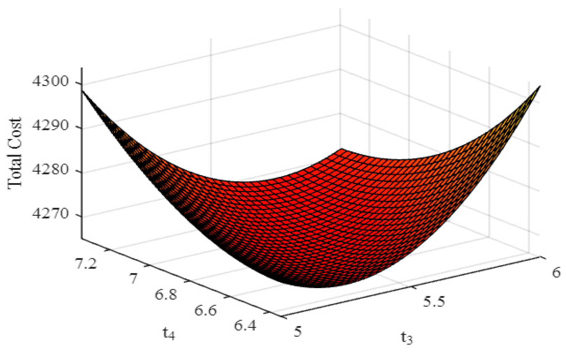
The convexity of the total cost function is depicted in Figure 2. We can estimate the optimal values of $t_4$ and $t_3$ using the software MATLAB. Our primary goal is to minimize the total cost function $TC(t_3,t_4)$, and the necessary conditions for doing so are as follows:

$$\frac{\partial }{\partial t_3}TC(t_3,t_4)=0 \mathrm{and}\frac{\partial }{\partial t_4}TC(t_3,t_4)=0$$

(23)

The optimal values $t_3^{*}$ and $t_4^{*}$ of $t_3$ and $t_4$ that satisfy the following necessary requirements of minimizing the profit function $TC\left(t_3,t_4\right)$ are

$$\frac{{\partial }^{2}TC(t_3,t_4)}{\partial {t_3}^2}>0, \frac{{\partial }^{2}TC(t_3,t_4)}{\partial {t_4}^2}>0 \mathrm{a}\mathrm{n}\mathrm{d}$$

$$\left(\frac{{\partial }^{2}TC(t_3,t_4)}{\partial {t_3}^2}\right)\left(\frac{{\partial }^{2}TC(t_3,t_4)}{\partial {t_4}^2}\right)-{\left(\frac{{\partial }^{2}TC(t_3,t_4)}{\partial {t_{3}t}_4}\right)}^2>0.$$

(24)

4. Numerical Example and Sensitivity Analysis

4.1. Numerical Example

For illustration purposes, we assume that the entire purchasing cost is prepaid in five equally spaced time points in advance to receive the ordered goods. That is $𝓃=5$. We study the system behavior in a particular environment, which is represented with the following parameters: $\mathcal{A}=22$; $𝒷=0.24$; $t_1=3$; $t_2=5; {\eta }_r=0.07$; ${\eta }_o=0.11$; $\xi =0.08$; ${\mathcal{O}}_1=900$; ${\mathcal{O}}_2=200$; ${\mathcal{P}}_1=82$; ${\mathcal{P}}_2=90$; ${\mathcal{H}}_r=10$; ${\mathcal{H}}_o=4$; ${\mathcal{D}}_r=9$; ${\mathcal{D}}_o=5.7$; ${\mathcal{C}}_s=8.7$; $\mathcal{M}=2$; ${\mathcal{I}}_{\mathcal{P}}=0.12$. Minimal total cost for the entire replenishment cycle in the above mentioned environment is determined as $TC=4265.149$ only if $t_3=5.5019$ and $t_4=6.845$ by using MATLAB code. The model suggests to the retailer to order $\mathcal{N}+{\mathcal{B}}_2=350$ items from the regular supplier and ${\mathcal{B}}_1=23$ items from the local supplier in order to satisfy the exigency. Figure 2 presents the total cost function of the inventory system.

4.2. Sensitivity Analysis

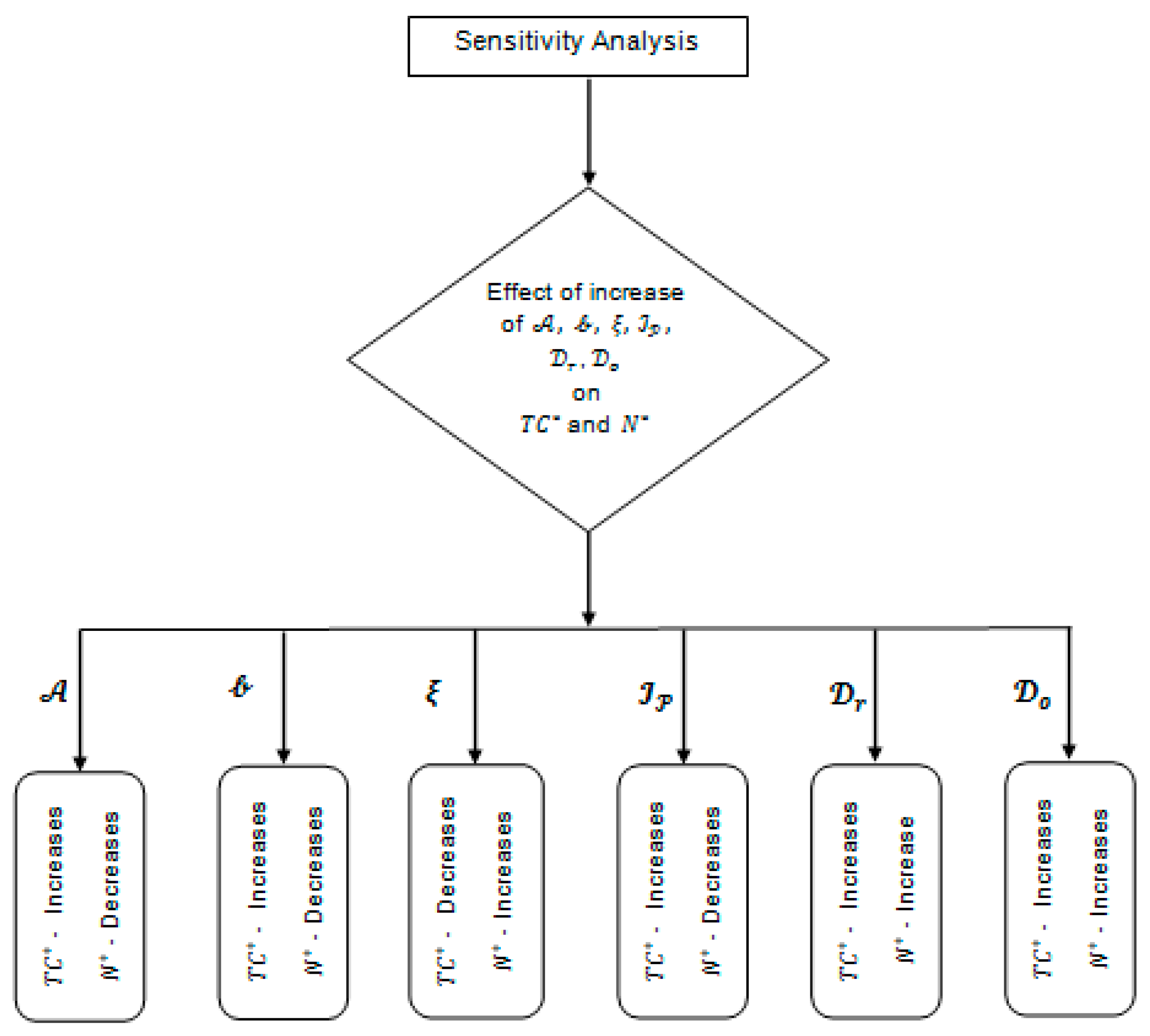
A mini map that represents the flow of the study of sensitivity analysis to observe changes in the optimal cost and the optimum ordering quantity by increasing the demand parameters, discount rate, interest rate and deterioration rates is given in Figure 3.

4.2.1. Effect of Changes in Demand Parameters $\mathcal{A}$ and $𝒷$ on Arriving Optimal Total Cost and Optimal Ordering Quantity

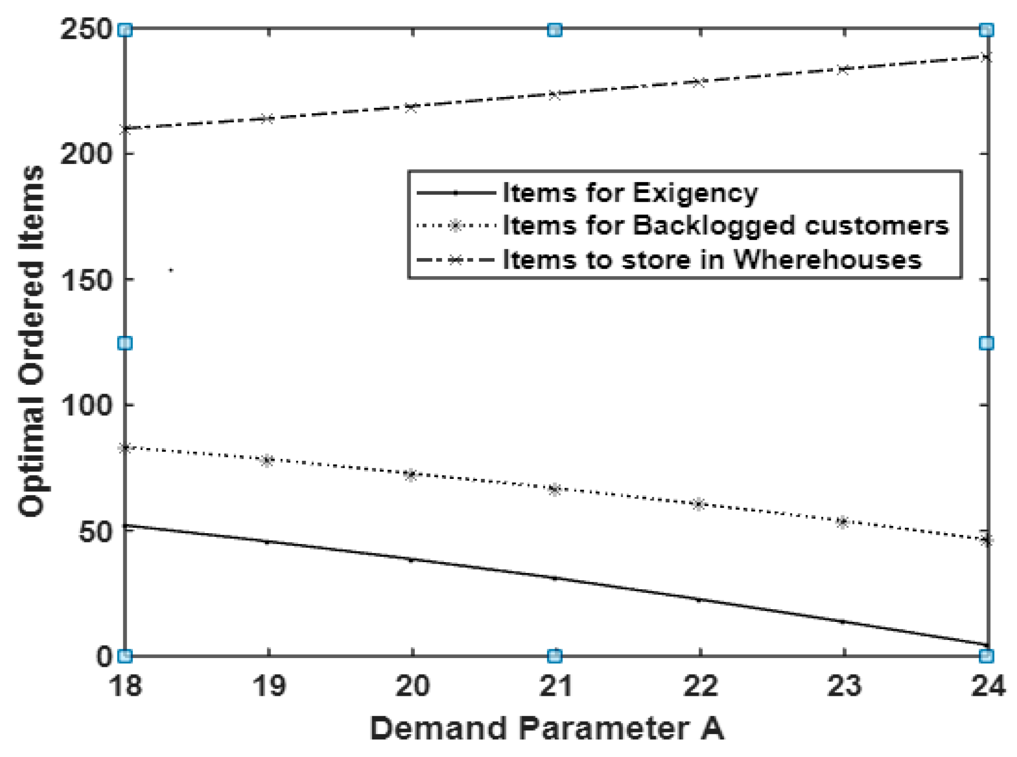
In the above-mentioned environment of illustration, we have $t_1=3$; $t_2=5; {\eta }_r=0.07$; ${\eta }_o=0.11$; $\xi =0.08$; ${\mathcal{O}}_1=900$; ${\mathcal{O}}_2=200$; ${\mathcal{P}}_1=82$; ${\mathcal{P}}_2=90$; ${\mathcal{H}}_r=10$; ${\mathcal{H}}_o=4$; ${\mathcal{D}}_r=9$; ${\mathcal{D}}_o=5.7$; ${\mathcal{C}}_s=8.7$; $\mathcal{M}=2$; ${\mathcal{I}}_{\mathcal{P}}=0.12$; $\mathcal{A}=22$; $𝒷=0.24$; We oscillate the parameter values $\mathcal{A}$ from 18 to 24 and $𝒷$ from $0.20$ to $0.26$. The effect on optimum cost, ordering quantity (both from regular and from local supplier) and length of stock out period is listed in

Table 2. The effect of changes in demand parameters $\mathcal{A}$ and $𝒷$ on arriving at optimal total cost and optimal ordering quantity.

$\mathcal{A}$	${\mathit{T}\mathit{C}}^{\mathit{*}}$	${{\mathcal{B}}_1}^{\mathit{*}}$	${\mathcal{N}}^{\mathit{*}}$
18	3781.457	52.1415	293.3051
19	3909.425	45.6701	292.5094
20	4032.769	38.6233	291.7275
21	4151.393	31.0630	290.8224
22	4265.149	22.5988	289.4653
23	4373.828	13.7031	287.7179
24	4477.146	4.4376	285.1487
$𝒷$
0.20	4028.958	48.5048	303.8589
0.21	4089.992	42.9597	300.6737
0.22	4149.960	36.6063	297.5752
0.23	4208.495	29.8260	294.1460
0.24	4265.149	22.5988	289.4653
0.25	4319.365	14.9037	284.3642
0.26	4370.436	05.7591	279.3016

. It is observed that an increase in $\mathcal{A}$ and $𝒷$ was positively correlated with the optimum total cost and negatively correlated with the ordering items both from regular and local suppliers. It is depicted in Figure 4 and Figure 5.

4.2.2. Effect of Changes in Interest Rate ${\mathcal{I}}_{\mathcal{P}}$ and Discount Rate $\xi$ on Arriving at Optimal Total Cost and Optimal Ordering Quantity

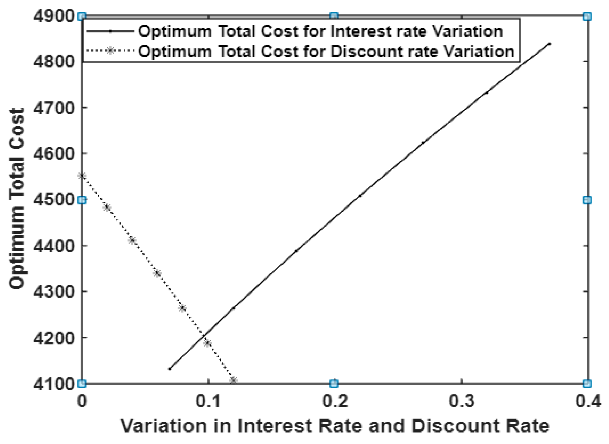
The variations in the interest rate and discount rates on compulsory complete prepayment option, influence on optimum total cost and optimum items ordered from both regular and local supplier with the following same environment for $\mathcal{A}=22$; $𝒷=0.24$; $t_1=3$; $t_2=5; {\eta }_r=0.07$; ${\eta }_o=0.11$; ${\mathcal{O}}_1=900$; ${\mathcal{O}}_2=200$; ${\mathcal{P}}_1=82$; ${\mathcal{P}}_2=90$; ${\mathcal{H}}_r=10$; ${\mathcal{H}}_o=4$; ${\mathcal{D}}_r=9$; ${\mathcal{D}}_o=5.7$; ${\mathcal{C}}_s=8.7$; $\mathcal{M}=2$ are observed. An increase in interest rate ${\mathcal{I}}_{\mathcal{P}}$ are positively correlated with the optimum total cost and negatively correlated with length of stock out period. An increase in discount rate $\xi$ is negatively correlated with optimum total cost and positively correlated with length of stock out period. It is displayed in

Table 3. The effect of changes in the interest rate ${\mathcal{I}}_{\mathcal{P}}$ and the discount rate $\xi$ on arriving at optimal total cost and optimal ordering quantity.

${\mathcal{I}}_{\mathcal{P}}$	${\mathit{T}\mathit{C}}^{*}$	${{\mathcal{B}}_1}^{*}$	${\mathcal{N}}^{\mathit{*}}$
0.07	4134.292	7.6836	290.3693
0.12	4265.149	22.5988	289.4653
0.17	4389.904	37.0620	288.1094
0.22	4509.268	50.6212	286.3015
0.27	4623.794	63.7285	284.0416
0.32	4733.918	76.3838	280.8778
0.37	4839.989	88.5872	277.2620
ξ
0.00	4553.632	56.0449	285.3976
0.02	4484.261	47.9094	286.7535
0.04	4413.137	39.7738	287.6574
0.06	4340.145	31.1863	289.0134
0.08	4265.149	22.5988	289.4653
0.10	4187.993	14.0112	289.9173
0.12	4108.489	4.5198	290.3693

and depicted in Figure 6. In particular, the order for exigency is increased while ${\mathcal{I}}_{\mathcal{P}}$ increases but it is decreased while $\xi$ increases and this is clear from Figure 7.

4.2.3. Effect of Changes in Deterioration Rate ${\mathcal{D}}_r$ and ${\mathcal{D}}_o$ on Arriving Optimal Total Cost and Optimal Ordering Quantity

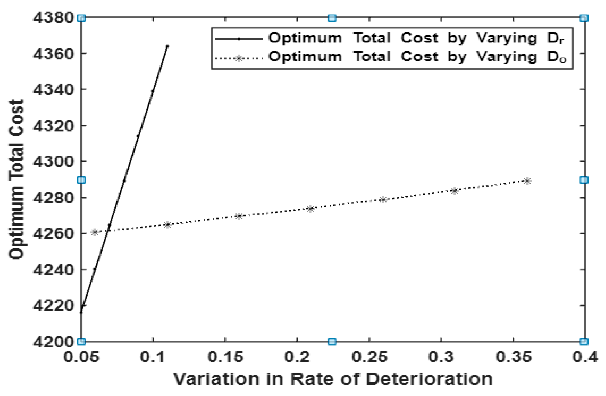
Effect of changes in deterioration rate, both in rental and own, where houses in optimum total cost, length of stock out period, ${\mathcal{N}}^{*}$ and ${{\mathcal{B}}_1}^{*}$ in the following environment $\mathcal{A}=22$; $𝒷=0.24$; $t_1=3$; $t_2=5; {\eta }_r=0.07$; ${\eta }_o=0.11$; $\xi =0.08$; ${\mathcal{O}}_1=900$; ${\mathcal{O}}_2=200$; ${\mathcal{P}}_1=82$; ${\mathcal{P}}_2=90$; ${\mathcal{H}}_r=10$; ${\mathcal{H}}_o=4$; ${\mathcal{C}}_s=8.7$; $\mathcal{M}=2$; ${\mathcal{I}}_{\mathcal{P}}=0.12$ are displayed in

Table 4. The effect of changes in deterioration rate ${\mathcal{D}}_r$ and ${\mathcal{D}}_o$ on arriving optimal total cost and optimal ordering quantity.

${\mathcal{D}}_{\mathit{r}}$	${\mathit{T}\mathit{C}}^{\mathit{*}}$	${{\mathcal{B}}_1}^{\mathit{*}}$	${\mathcal{N}}^{\mathit{*}}$
0.05	4216.542	17.1751	280.3549
0.06	4240.780	19.8869	284.8904
0.07	4265.143	22.598	289.4653
0.08	4289.658	25.3106	294.5327
0.09	4314.313	28.4744	299.1893
0.10	4339.122	31.1863	303.8884
0.11	4364.091	33.8981	309.0827
${\mathcal{D}}_{\mathit{o}}$
0.06	4260.719	22.1468	289.0134
0.11	4265.149	22.598	289.4653
0.16	4269.578	23.0507	290.3693
0.21	4274.131	23.5027	290.8213
0.26	4278.918	24.4067	291.2732
0.31	4284.034	24.8586	291.7252
0.36	4289.566	25.3106	292.6292

. An increase in deterioration rates ${\mathcal{D}}_r$ and ${\mathcal{D}}_o$, affects and increases both $t_3^{*}$ and $t_4^{*}$; in turn, it causes an increase in ${TC}^{*}$, ${\mathcal{N}}^{*}$, ${{\mathcal{B}}_1}^{*}$. It is depicted in Figure 8 and Figure 9.

5. Results, Discussions and Suggestions

Firstly, it is considered the effect of changes on the demand parameters $\mathcal{A}$ and $𝒷$. The first parameter is the magnification part of the ramp-type demand whose increase results in huge positive changes in the demand pattern, and the second parameter is the exponential power parameter $𝒷$ whose rise contributes to a little less increase in the overall demand rate. In a retailer’s point of view, to optimize the total cost in their business, the optimal ordering quantity should be analyzed based on the arrival of the demand pattern. As such, first we observed the optimal ordering quantity with respect to the increased demand parameter values, which are listed in Table 2 and supported by Figure 4 and Figure 5. Under the considered environment, as the demand rates increase, simultaneously the optimum total cost is increased, but at the same time the optimal ordering quantity is decreased. Optimum ordered items for an exigency are also decreased.

Suggestion: It is suggested that the retailer can predict their optimum total cost as per the capacity of their inventory storage facility and may decide the optimal interval of backlog and the number of exigency order items in order to attain the optimum total cost. If the retailer is more attentive and wants to reduce the number of purchase items for exigency, then it may be opt for him to order ${\mathcal{N}}^{*}=285$ items to achieve so.

In the study of inventory models with prepayment options, the two parameters, namely the discount rate $\xi$ for prepayment and the interest rate ${\mathcal{I}}_{\mathcal{P}}$ on the amountwe pay in advance, are essential ingredients for any retailer’s decision-making processes on optimizing the total cost. How the increased rate of discount and interest will influence the optimum total cost and total ordering quantity is displayed in Table 3. First, the behavior of optimal total cost by increasing the interest rate and discount rates is depicted in Figure 6. We may observe that the optimal total cost is increased while increasing the interest rate and it is decreased for the increase in the discount rate. It is true in nature and it seems that the model behaves well. Secondly, the behavior of optimal total ordering items for exigency by increasing the interest rate and discount rates is depicted in Figure 7. We may observe that the optimal total ordering of items for exigency also increased while increasing the interest rate and it decreased for the increase in the discount rate.

Suggestion: Table 3 helps the retailer to choose the suitable supplier with whom he may get the higher discount for his selection of advance payment policy to optimize his total cost. For example, in the above considered environment, if the retailer chooses the supplier who offers the discount rate of $\xi =0.12$, then their optimum total cost ${TC}^{\mathit{*}}$ is $4108$ units of money. In the same way, the retailer may take the prepayment option as per the interest rate to optimize not only the total cost but also the total exigency order and total usual order quantity too.

Product obsolescence is inevitable on handling sensitive items such as medicinal products, chemical products, vegetables, fruits, meat, and donated blood pouches. In the present study, the items in both warehouses may get deteriorate during the course of selling phase. If the deterioration rates ${\mathcal{D}}_r$ and ${\mathcal{D}}_o$ of items in $RW$ and $OW$ are increased, then the range of its influence in arriving at the optimal total cost and optimal ordering of items and items to be purchased for satisfying exigency are displayed in Table 4. We may observe that the increase in deterioration rate of items in $RW$ is more sensitive and increases the optimum total cost of the cycle more drastically than the increase in ${\mathcal{D}}_o$ which is depicted in Figure 8. We can observe the same effect on optimum order for exigency too and it is depicted in Figure 9.

Suggestion: If the retailer wants to avoid more purchases for exigency, his choice has to be ${\mathcal{D}}_r=0.05$ in the above-mentioned environment, so that the optimum order for exigency will be $17$ items; instead, if ${\mathcal{D}}_r=0.11$, then the optimum order for exigency will be increased. At the same time, the optimal total cost will be raised from $4217$ units of money nearly to $4364$ units of money nearly. Table 4 suggests the retailer to optimize the total cost by identifying the product for sales based on its deterioration rate.

6. Conclusions

In this study, we have constructed a two-warehouse inventory model of constantly deteriorating items. The current study emphasizes the effect of the retailers’ N-phase prepayment option, and the purchasing of items from a local supplier to manage exigency in order to arrive at an optimal total cost of the replenishment cycle. An analytical solution to this model was provided to reduce overall inventory costs with sensitivity analysis. Moreover, the ideal order amount, replenishment cycle length, backorder quantities and backlog duration have been identified. The effect of the model is tested in a particular environment for validation and covers the effect of changes in demand parameters, interest rate, and discount rate and deterioration rates on arriving at an optimal total cost and optimal ordering quantity. Appropriate suggestions are recommended to the retailer in Section 5. The present work has a wide scope for extending it by including with items’ re-do facility, integrated production unit, late payment options and so on.

References

1. Hing-LingLau, A.; Lau, H.-S. Decision models for single-period products with two ordering opportunities. Int. J. Prod. Econ. 1998, 55, 57–70. [Google Scholar] [CrossRef]
2. SanJosé, L.A.; Sicilia, J.; García-Laguna, J. The lot size-reorder level inventory system with customers impatience functions. Comput. Ind. Eng. 2005, 49, 349–362. [Google Scholar] [CrossRef]
3. Jaggi, C.K.; Goel, S.K.; Tiwari, S. Two-warehouse inventory model for non-instantaneous deteriorating items under different dispatch policies. Investig. Oper. 2018, 38, 343–365. [Google Scholar]
4. Taleizadeh, A.A.; Tavassoli, S.; Bhattacharya, A. Inventory ordering policies for mixed sale of products under inspection policy, multiple prepayment, partial trade credit, payments linked to order quantity and full backordering. Ann. Oper. Res. 2020, 287, 403–437. [Google Scholar] [CrossRef] [Green Version]
5. Taleizadeh, A.A. An EOQ model with partial backordering and advance payments for an evaporating item. Int. J. Prod. Econ. 2014, 155, 185–193. [Google Scholar] [CrossRef]
6. Tavakoli, S.; Taleizadeh, A.A. An EOQ model for decaying item with full advanced payment and conditional discount. Ann. Oper. Res. 2017, 259, 415–436. [Google Scholar] [CrossRef]
7. Mondal, R.; Das, S.; Das, S.C.; Shaikh, A.A.; Bhunia, A.K. Pricing strategies and advance payment-based inventory model with partially backlogged shortages under interval uncertainty. Int. J. Syst. Sci. Ope. r. Logist. 2022, 10, 1–25. [Google Scholar] [CrossRef]
8. Khanam, Z.; Ali, A. Inventory Model with Advance Payment and Backlogging. J. Mech. Contin. Math. Sci. 2019, 14, 558–569. [Google Scholar] [CrossRef]
9. Taleizadeh, A.A.; Pentico, D.W.; Jabalameli, M.S.; Aryanezhad, M. An economic order quantity model with multiple partial prepayments and partial backordering. Math. Comput. Model. 2013, 57, 311–323. [Google Scholar] [CrossRef]
10. Sarkar, B.; Sarkar, S. An improved inventory model with partial backlogging, time varying deterioration and stock-dependent demand. Econ. Model. 2013, 30, 924–932. [Google Scholar] [CrossRef]
11. Panda, S.; Senapati, S.; Basu, M. Optimal replenishment policy for perishable seasonal products in a season with ramp-type time dependent demand. Comput. Ind. Eng. 2008, 54, 301–314. [Google Scholar] [CrossRef]
12. Khakzad, A.; Gholamian, M.R. The effect of inspection on deterioration rate: An inventory model for deteriorating items with advanced payment. J. Clean. Prod. 2020, 254, 120117. [Google Scholar] [CrossRef]
13. Skouri, K.; Konstantaras, I.; Papachristos, S.; Ganas, I. Inventory models with ramp type demand rate, partial backlogging and Weibull deterioration rate. Eur. J. Oper. Res. 2009, 192, 79–92. [Google Scholar] [CrossRef]
14. Agrawal, S.; Banerjee, S.; Papachristos, S. Inventory model with deteriorating items, ramp-type demand and partially backlogged shortages for a two warehouse system. Appl. Math. Model. 2013, 37, 8912–8929. [Google Scholar] [CrossRef]
15. Chakraborty, D.; Jana, D.K.; Roy, T.K. Two-warehouse partial backlogging inventory model with ramp type demand rate, three-parameter Weibull distribution deterioration under inflation and permissible delay inpayments. Comput. Ind. Eng. 2018, 123, 157–179. [Google Scholar] [CrossRef]
16. Shi, Y.; Zhang, Z.; Zhou, F.; Shi, Y. Optimal ordering policies for a single deteriorating item with ramp-type demand rate under permissible delay inpayments. J. Oper. Res. Soc. 2018, 70, 1–21. [Google Scholar] [CrossRef]
17. Mandal, B.; Pal, A.K. Order level inventory system with ramp type demand rate for deteriorating items. J. Interdiscip. Math. 1998, 1, 49–66. [Google Scholar] [CrossRef]
18. Panda, S.; Saha, S.; Basu, M. An eoq model with generalized ramp-type demand and weibull distribution deterioration. Asia-Pac. J. Oper. Res. 2007, 24, 93–109. [Google Scholar] [CrossRef]
19. Manna, S.K.; Chaudhuri, K.S. An EOQ model with ramp type demand rate, time dependent deterioration rate, unit production cost and shortages. Eur. J. Oper. Res. 2006, 171, 557–566. [Google Scholar] [CrossRef]
20. Karmakar, B. Inventory models with ramp-type demand for deteriorating items with partial backlogging and time-varing holding cost. Yugosl. J. Oper. Res. 2014, 24, 249–266. [Google Scholar] [CrossRef] [Green Version]
21. Teng, J.-T.; Cárdenas-Barrón, L.E.; Chang, H.-J.; Wu, J.; Hu, Y. Inventory lot-size policies for deteriorating items with expiration dates and a dvance payments. Appl. Math. Model. 2016, 40, 8605–8616. [Google Scholar] [CrossRef]
22. Rahimi-Ghahroodi, S.; AlHanbali, A.; Vliegen, I.M.H.; Cohen, M.A. Joint optimization of spare parts inventory and service engineers staffing with fullbacklogging. Int. J. Prod. Econ. 2019, 212, 39–50. [Google Scholar] [CrossRef]
23. Janssen, F.; deKok, T.A. Two-supplier inventory model. Int. J. Prod. Econ. 1999, 59, 395–403. [Google Scholar] [CrossRef] [Green Version]
24. Majumder, P.; Bera, U.K.; Maiti, M. An EPQ model for two-warehouse in unremitting release pattern with two-level trade credit period concerning both supplier and retailer. Appl. Math. Comput. 2016, 274, 430–458. [Google Scholar] [CrossRef]
25. Shu, J. An Efficient Greedy Heuristic for Warehouse-Retailer Network Design Optimization. Transp. Sci. 2010, 44, 183–192. [Google Scholar] [CrossRef]
26. Teo, C.-P.; Shu, J. Warehouse-Retailer Network Design Problem. Oper. Res. 2004, 52, 396–408. [Google Scholar] [CrossRef]
27. Chih-Te, Y.; Ouyang, L.-Y.; Wu, K.-S.; Yen, H.-F. An inventory model with temporary price discount when lead time links to order quantity. J. Sci. Ind. Res. 2010, 69, 180–187. [Google Scholar]
28. Thilagavathi, R.; Viswanath, J.; Cepova, L.; Schindlerova, V. Effect of Inflation and Permitted Three-Slot Payment on Two-Warehouse Inventory System with Stock-Dependent Demand and Partial Backlogging. Mathematics. 2022, 10, 3943. [Google Scholar] [CrossRef]
Figure 1. Graphical representation of the model.
Mathematics 11 01728 g001
Figure 2. Total cost function of the inventory system.
Mathematics 11 01728 g002
Figure 3. Flow of the sensitivity analysis.
Mathematics 11 01728 g003
Figure 4. The effect of changes in demand parameter A on optimal ordering items.
Mathematics 11 01728 g004
Figure 5. The effect of changes in demand parameter 𝒷 on optimal ordering items.
Mathematics 11 01728 g005
Figure 6. The effect of changes in the interest rate I P and the discount rate ξ on arriving at optimal total cost.
Mathematics 11 01728 g006
Figure 7. The effect of changes in the interest rate I P and discount rate ξ on arriving at optimal order for exigency.
Mathematics 11 01728 g007
Figure 8. The effect of changes in deterioration rates D r and D o on optimal total cost.
Mathematics 11 01728 g008
Figure 9. The effect of changes in deterioration rates D r and D o on optimal order for exigency.
Mathematics 11 01728 g009