Abstract
Core acquisition is essential to the success of the remanufacturing business. The value of sorting and grading cores into nominal-quality classes has been certified in industry and academia. In this paper, we investigate how many unsorted cores of uncertain quality should be acquired and how many sorted cores should be remanufactured by a third-party remanufacturer (3PR) before the demand is realized. We first develop analytically tractable solutions to the acquisition and production model under deterministic demand, and then we extend it to the model under the stochastic demand by fully characterizing the structure of the optimal policy. Subsequently, we investigate the impact of core quality fraction uncertainty on the solutions. Finally, numerical analyses are conducted to further verify the proposed models. The results are as follows. First, the optimal quantity of acquisition/production and minimum expected profit increase with an increase in the selling price and decrease with an increase in the uncertainty of demand and acquisition cost. Second, the optimal production quantity does not decrease in acquisition quantity, and the rate of utilization of the recycled parts (the ratio of production quantity to acquisition quantity) increases with a decrease in the acquisition cost. Third, the growth stage is most profitable stage, so the remanufacturers should pay more attention to remanufacturing activities early in the life of products. The proposed models and solutions can not only solve the core acquisition and production problem in remanufacturing, but also solve the combinatorial optimization problem.
MSC:
90-10
1. Introduction
As a mode of environmental protection and energy saving in the context of production, remanufacturing has attracted the attention of enterprises and governments all over the world [1,2,3]. An increasing number of original equipment manufacturers use remanufacturing along with manufacturing to satisfy market demands with competitive prices and environmentally friendly production, e.g., Caterpillar, ReCellular, Boeing, Deere, and Sony. However, remanufacturing not only faces the same market uncertainties as traditional manufacturing, but also encounters the variation inherent in the condition of used products. To be more precise, the supply of raw materials is relatively stable and their quality is uniform in traditional manufacturing, whereas the supply and quality of recycled materials are usually uncertain in remanufacturing [4,5,6,7,8,9].
For the above reasons, supply-side management becomes more complex in remanufacturing than in manufacturing, which is a key input to assess the economic attractiveness of reuse activities [5]. Researchers have pointed out the importance of issues related to core acquisition, and a growing number of studies have dealt with quantitative decisions in this domain [10,11,12,13]. Ferguson et al. [14] have shown that the firm does not remanufacture a unit with a lower grade of quality before one with a higher grade is out of stock; in other words, the firm always remanufactures the higher-quality grade first after the cores have been acquired and sorted. In other words, for a given acquisition quantity, the cost of production in remanufacturing is a piecewise-linear convex function.
This study is motivated by the work of Mutha, Bansal, and Guide [12], who investigated whether a third-party remanufacturer (3PR) should acquire used products or cores with uncertain levels of quality in bulk or those with known levels of quality in sorted grades, and Mutha et al. [15], who studied inter-firm transactions for buying and selling used graded products with analytically tractable models. We consider the scenario in which a 3PR acquires used products with unknown levels of quality and sorts them into different grades to satisfy the demand. We also develop models to determine the optimal quantity of products to acquire and produce. Similar to the work conducted by Mutha, Bansal, and Guide [12] and Mutha, Bansal, and Guide [15], we investigate the policy of the core acquisition of 3PRs that remanufacture products with a high time value of money, i.e., products that become obsolete quickly and whose inventory loses value quickly. To be profitable in this environment, a 3PR needs to be efficient to avoid the risk of a depreciation of the inventory while being responsive to uncertain demands [12]. Previous research on this topic [9,16,17,18,19] has not focused on developing an analytically tractable solution. We establish a model of acquisition and production under deterministic demand, generalize it to scenarios involving stochastic demand, and provide an analytically tractable solution for it.
The contributions of this paper are as follows. For core acquisition management, we establish models on the optimal acquisition/production of unsorted/sorted used products for independent remanufacturing by giving analytically tractable solutions. For inventory management, we characterize the structure of the optimal policy by using a quantity-dependent piecewise-linear convex cost. The proposed models and solutions not only solve the problems of core acquisition and production in remanufacturing, but can also be used to solve combinatorial optimization problems [20], e.g., piecewise -linear, unsplittable, multi-commodity flow problems [21], and network design and routing problems [22].
The remainder of this paper is organized as follows. We review the related literature in Section 2. Section 3 characterizes the optimal acquisition and production policies for remanufacturing under deterministic and stochastic demands. Section 4 analyzes the impact of core quality fraction uncertainty. Section 5 presents a case study to verify the validity of the proposed models and discusses their sensitivity to parametric changes. The main findings and managerial insights of this study are summarized in Section 6, as well as some highlights of possible directions for future research.
2. Literature Review
This paper is most closely related to two streams of literature: core acquisition in remanufacturing operations and inventory–production control with a piecewise-linear convex cost. For a thorough review of academic work on core acquisition in remanufacturing, we refer interested readers to Atasu et al. [23]; Wei, Tang, and Sundin [7]; Jena and Sarmah [24]; and Peng et al. [25].
In the streams of core acquisition management, Guide [4] provided the first step in research on the management of used product acquisition by providing an overview of current practices. He claimed that the manager should take actions that consistently reduce the inherent variance in a remanufacturing environment. To address the inherent variance in recycled products and uncertainty in the demand for them, previous studies have explored mitigation strategies from different perspectives, e.g., product design [26,27], channel selection [28,29,30,31,32], acquisition quantity [33,34,35], price [36,37,38,39], timing [12,40], lot sizing [41], quality information [36,42,43], and grading [14,43,44], among others. In terms of quality grading, Aras et al. (2004) investigated the issue of the stochastic nature of product returns and identified conditions under which quality-based categorization is the most cost-effective. Ferguson, Guide, Koca, and Souza [14] further exhibited the value of quality grading in remanufacturing by explicitly considering quality-related information in deciding which returned products to remanufacture or dispose of. In addition, many studies have provided a greater understanding of the effects of quality grading in remanufacturing systems from other perspectives, such as network design and configuration [45,46], and optimizing the lot size and scheduling [6,47]. Studies on acquisition according to the time of grading can be divided into three main categories: pre-purchase grading [10,15,48], post-purchase grading [9,17,49], and hybrid grading [12]. This work focuses on post-purchase grading, considers the situation when a buyer acquires used products of unknown quality and sorts them into different grades, and develops models to determine the optimal number of products to acquire and manufacture for the remanufacturer.
The second stream of related research focuses on inventory–production control with a piecewise-linear convex cost. Research on inventory systems with a convex and variable cost of production can be traced back to the study by Karlin [50]. Recently, Lu and Song [51] characterized the optimal inventory control policy for a periodic review inventory control system with a fixed cost and a convex variable cost. Caliskan-Demirag et al. [52] and Li et al. [53] considered a case in which the cost of production was a step function of the quantity of production. Sillanpää et al. [54] proposed the optimal procurement decisions with a well-designed contract when the shortage costs of individual periods are piecewise-linear. Ardestani-Jaafari and Delage [55] examined the robust optimization of sums of piecewise-linear functions. Fortz, Gouveia, and Joyce-Moniz [21] considered multi-commodity flow problems with unsplittable flows and piecewise-linear routing costs. Lu et al. [56] conducted a periodic review-based inventory control problem with a general piecewise-linear cost. However, all the above studies assumed that the piecewise-linear convex cost of production is exogenously given, rather than a constituting decision, whereas it is determined by the quantity of acquisition in this study. We contribute to the stream of research on policies for inventory production with a quantity-dependent piecewise-linear convex cost of production, where the length of each piecewise segment depends on the quantity of products with the corresponding quality, added in order from the highest-quality grade to the worst.
The works most closely related to this one are conducted by Teunter and Flapper [9] and Mutha, Bansal, and Guide [12]. Teunter and Flapper [9] studied acquisition and remanufacturing decisions under uncertain-quality fractions of the core. With deterministic demand, they derived a simple closed-form expression for the total expected cost. Under uncertain demand, they presented optimal newsboy-type solutions for the optimal remanufacture-up-to levels and an approximate expression for the total expected cost, given the quantity of acquired cores. Mutha, Bansal, and Guide [12] investigated whether a 3PR should acquire used products or cores of uncertain quality levels in bulk or those with known quality levels in sorted grades, and whether to acquire and remanufacture cores before the demand has been realized (planned acquisition) or after it (reactive acquisition), or on both occasions (sequential acquisition). However, Teunter and Flapper [9] derived an approximate expression for the total expected cost under uncertain demand. Mutha, Bansal, and Guide [12] gave a complicated first-order functional expression that can be used to solve for the optimal quantity of acquisition but does not determine this quantity. Based on the studies above, we develop the models to derive analytically tractable solutions for models of unsorted core acquisition in this study. In short, this study makes two contributions to the literature. We establish optimal acquisition/production models of unsorted/sorted used products for core acquisition management in independent remanufacturing by proposing analytically tractable solutions. We characterize the structure of the optimal policy for managing inventory production in a system with a quantity-dependent piecewise-linear convex cost of production.
3. The Model
The remanufacturer acquires unsorted used products and remanufactures them before the demand has been realized. We develop an optimal acquisition and production model with a linear acquisition cost and a quantity-dependent piecewise-linear convex production cost, while considering uncertainty in demand. The sequence of events is as follows. First, the remanufacturer acquires unsorted cores and classifies them into grades according to the quality levels. Second, the remanufacturer converts units of sorted cores into finished products by incurring a production cost of for each unit of grade . Finally, the demand is realized and the remanufacturer attempts to meet the demand, generating revenue for each unit sold.
The assumptions and parameters are as follows:
Assumptions:
A1. Consistent with practice in the remanufacturing industry, grades in which used products are sorted are exogenously defined [14,38].
A2. All remanufactured products have the same specifications before sale [16,17].
A3. The remanufacturer acquires unsorted used products at a fixed price per unit [12,15].
Parameters:
—quality category, ;
—the acquisition quantity of cores;
—the proportion of quality-i cores, where ;
—the unit remanufacturing cost for quality-i cores, where ;
—the acquisition cost per return;
—the sale price per remanufactured product;
—the production quantity;
—the demand quantity.
The demand for the finished products is uncertain with respect to a cumulative density function and a probability density function , where for all and otherwise. The function that aims to maximize profits for the remanufacturer can be expressed by Equation (1):
The first term on the right-hand side represents the revenue raised from selling remanufactured products; the second term represents the production cost, which is jointly determined by the quantities of acquisition and production ; and the third term represents the acquisition cost.
Following Ferguson, Guide, Koca, and Souza [14], we assume that the firm classifies cores based on quality, , as follows: cores with are labeled for remanufacturing and those with are labeled as scrap for part harvesting. The range is further divided into slices, , in order to classify the re-manufacturable cores into quality grades .
According to Ferguson, Guide, Koca, and Souza [14], remanufacturing production activities always start from the item with the highest-quality grade and remanufactures until no items are left in the current quality grade. As shown in Figure 1, the production cost can be expressed by Equation (2):
where denotes the cumulative ratio from quality-1 to quality-i, , , , , for all , and is the indicator function.
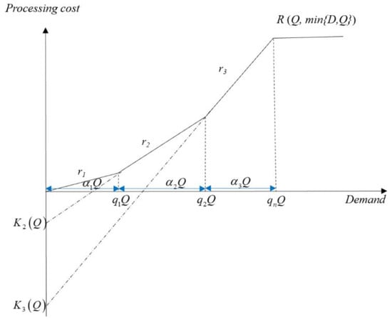
Figure 1.
The production cost when the cores are divided into three categories.
We assume that all quality levels are marginally profitable because the ratio of grades of quality is fixed, which will be relaxed in Section 4. This does not affect the final conclusion, even if a certain percentage of cores is not marginally profitable or cannot be remanufactured. Based on the above analysis of remanufacturing production costs, we first give Lemma 1.
Lemma 1.
- a.
- is a piecewise-linear convex function and increasingly continuous in the interval for a given acquisition quantity .
- b.
- is non-increasing in for a given production quantity .
The proof of Lemma 1 and the proofs of the other Lemmas and propositions are given in the Appendix A.
We now consider the model with deterministic demand and generalize it to one with stochastic demand.
3.1. Special Case: Demand Is Deterministic
The optimal production quantity is always equal to the demand when the demand is known with the assumption that all quality levels are marginally profitable, given that . The objective function (1) can then be expressed by Equation (3):
According to Lemma 1(b), the production cost is non-increasing in for a given production quantity . At the same time, the acquisition cost is increasing in . We can thus obtain Lemma 2.
Lemma 2.
The total cost function is discretely convex in when the demand is fixed.
For the given profit function , its first difference is . By this time, it is easy to obtain the characteristics of the profit function by Proposition 1.
Proposition 1.
The profit function is discretely concave in when the demand is fixed.
Based on properties of the total cost and profit functions given in Lemma 2 and Proposition 1, we aim to optimize the acquisition quantity after the demand has been determined. Suppose that the quantity demanded is in the interval when the purchase quantity is , and the quantity demanded is in the interval when the purchase quantity is , i.e., and . At this point, we can then obtain the first difference function of the total costs below.
Obviously, the larger the acquisition quantity, the smaller when the demand/production quantity is deterministic, i.e., because is less than . Thus, we can derive the following two inequalities:
In other words, . Given any acquisition quantity , the upper and lower bounds of the first difference in the total cost are and , respectively. If , then and ; in other words, to increase the marginal profit, the acquisition quantity needs to be increased. If , then and ; in other words, the marginal profit decreases with a reduction in acquisition quantity; otherwise, it can vary.
For the sake of brevity, let , . We then have . is the marginal acquisition cost and is the marginal savings in production costs when the production quantity is in the interval. In other words, is the marginal cost and is the marginal profit when the production quantity is in the interval.
As described in Proposition 1, the profit function is discretely concave in when the demand is fixed. The optimal acquisition quantity must satisfy the following conditions: and . Consequently, the optimal acquisition quantity is for and when and .
Similarly, , ,, and if . Consequently, the optimal acquisition quantity can be any value on the interval when .
If , then () is always negative (positive), which means the marginal profit is positive. With the assumption that the remanufacturing activities is always profitable, the re-manufacturable quantity equals the demand, as shown by .
The optimal acquisition quantity can be obtained by Proposition 2 when the demand is deterministic.
Proposition 2.
When the demand is deterministic,
- a.
- the optimal acquisition quantity is if and ;
- b.
- the optimal acquisition quantity can be arbitrarily determined on the interval if ;
- c.
- the optimal acquisition quantity is if .
Proposition 2 reveals that the optimal acquisition quantity can be obtained at the interval where the marginal profit is equal to 0 if it exists (Proposition 2(b)) and the optimal acquisition quantity of re-manufacturable is equal to the demand when the acquisition cost is high enough, given that (Proposition 2(c)). Otherwise, the optimal acquisition quantity can be obtained by looking for the boundary values where and (Proposition 2(a)).
3.2. Demand Is Stochastic
We will answer two questions in this section: how many unsorted cores need to be acquired and how many sorted cores need to be remanufactured into finished products, which is dependent on the acquisition quantity found in the first step. We solve for the optimal quantities of production and acquisition by backward derivation. We start by optimizing the quantity of production with a given acquisition quantity, and then further explore the optimal acquisition quantity. In the second stage, the quantity of acquisition is given, and the objective problem becomes one of inventory production with a piecewise -linear convex cost. This has been discussed by Lu and Song [51] and Lu, Song, and Yang [56].
Let , and define . Then, decreases in . This implies that because is discretely convex. can be interpreted as the optimal production level if the unit cost of production is , . It is then easy to demonstrate that . Thus, can be obtained by letting ; thus, . Let ; it monotonically increases in and monotonically decreases in . For simplicity but not generality, let .
Based on the method given in Lu and Song [51], we can obtain the optimal production quantity in the second stage by Proposition 3.
Proposition 3.
For a given acquisition quantity, the optimal production quantity is if , for , and the optimal production quantity is if for ; thus, .
For any given acquisition quantity, we can find the optimal production quantity according to Proposition 3, and this is a one-to-one relationship. For and , we can obtain Lemma 3 by using the result given by Proposition 3.
Lemma 3.
The optimal production quantity does not decrease in acquisition quantity .
We analyze the optimization of the acquisition quantity in the first stage after analyzing the characteristics of the production of the second stage. To obtain the optimal quantity of acquisition, we first analyze the properties of the first difference in the profit function by Lemma 4.
Lemma 4.
The first difference in does not increase in ; thus,
According to Lemma 4, the profit function is piecewise-differentiable and does not increase. We can thus obtain Proposition 4.
Proposition 4.
The profit function is discretely concave with respect to the acquisition quantity .
According to Proposition 4, the profit function is discretely concave in the acquisition quantity , so the optimal acquisition quantity is the one (those) which satisfies the following conditions: and .
If , then , according to Lemma 4 and Proposition 4, and the optimal acquisition quantity is in the first interval . Consequently, we can obtain the optimal acquisition quantity by letting , which is .
Similarly, if and , the optimal acquisition quantity is in the interval , so the optimal acquisition quantity can be obtained by letting , which is . If , the optimal acquisition quantity can be any value in the interval .
Consequently, we can derive the optimal acquisition quantity using Proposition 5.
Proposition 5.
When the demand is stochastic,
- a.
- the optimal acquisition quantity is if ;
- b.
- the optimal acquisition quantity is , where satisfies the following two conditions: and ;
- c.
- the optimal acquisition quantity is if .
Proposition 5 analytically gives tractable solutions to obtain the optimal acquisition quantity as long as we know the sum of and , where is the first difference in the fixed production cost of quality , given that . At the same time, Proposition 3 describes a simple method that can be used to obtain the optimal production quantity for the acquisition quantity given in the first stage, which only depends on and , .
We analytically provide tractable solutions to the problems of core acquisition and production by considering stochastic demands. Next, we will further explore the impact of core quality fraction uncertainty 0 in Section 4.
4. The Impact of Core Quality Fraction Uncertainty
In this section, we explicitly consider the cases when the quality of acquired cores is uncertain. We only know the probability that an acquired core is of quality-i is . Consider a collection lot of cores. Let denote the order statistics of the cores, ordered by condition. According to Evans et al. [57], the probability density function of can be expressed by Equation (4)
The formula for the probability density function of is a direct result of the following observation. For the order statistic to equal , there must be values less than or equal to and values greater than or equal to , where and . The other values must be equal to . The cumulative density function procedure is used to determine the probability of obtaining a value less than or equal to , the survivor function procedure is used to determine the probability of obtaining a value greater than or equal to , and the probability density function procedure is used to determine the probability of obtaining the value . The multinomial coefficient expresses the number of combinations resulting from a specific choice of and . Consequently, the order statistical probability of obtaining the quality-i cores is .
So far, we can use the methods given in Proposition 5 to optimize acquisition decisions with substituting order statistical probability for the fixed proportion . Subsequently, the optimal production quantity can be achieved according to Proposition 3 after the core quality fractions are realized.
5. Numerical Study
In this section, we perform a numerical study to verify the analytical results above and intuitively illustrate them based on data from ReCellular reported by Mutha, Bansal, and Guide [12]. The selling price is , the cost of acquisition is , and the uncertainty in demand is normal with and . The cores are sorted into four grades; the costs of remanufacturing are , , , and ; and their proportions are , , , and , respectively.
5.1. Results and Discussion
Table 1 shows the values of the functions directly related to the solution: , ,, and . According to Proposition 5, the optimal acquisition quantity is because and .

Table 1.
Numerical analyses.
As shown in Table 2, ; thus, according to Proposition 3, the optimal production quantity is . Consequently, the expected profit is .
Table 2.
The value of and when the acquisition quantity is .
To clarify the characteristics of the problem, we show the trends of change in the optimal production quantity and expected profits in Figure 2. The blue area represents the trend of the optimal production quantity and the orange line represents the maximum expected profit for a given acquisition quantity. We also mark the position of , , and in blue, red, and yellow in Figure 2, which can help readers understand the characteristics of the optimized problem more intuitively. As demonstrated in Proposition 3, the optimal production quantity is if and the optimal production quantity is if . As demonstrated in Lemma 3 and Proposition 4, the optimal production quantity is piecewise-non-decreasing with respect to acquisition quantity , and the profit function is discretely concave with respect to the acquisition quantity . Specifically, the optimal production quantity is equal to the acquisition quantity when the acquisition quantity is not greater than . The optimal production quantity does not change whereas the expected profit continues to decrease when the acquisition quantity exceeds .
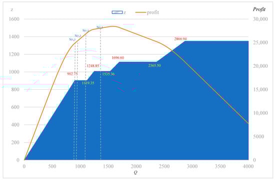
Figure 2.
The optimal production quantity and expected profit .
5.2. Sensitivity Analysis
We also analyze the sensitivity of the parameters to explore the effect of the unit acquisition cost on the results. We change it from 0 to 23.37 in steps of 2.895. The results are shown in Table 3 and Figure 3. The optimal quantity of acquisition/production and the minimum expected profit decrease as the unit acquisition cost increases. Note that the optimal quantity of production is always the product of the optimal quantity of acquisition and because , which can be deduced from Proposition 3. As increases, the rate of utilization of cores increases from to , which means that a lower cost of acquisition can improve the expected profit and quantity of the acquisition of remanufacturers while improving the rate of utilization of the recycled parts.
Table 3.
The result for various unit acquisition costs .
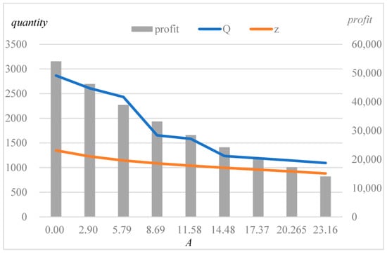
Figure 3.
The result for various unit acquisition costs .
Similarly, we analyze the effects of the selling price and the standard deviation of the demand on the results, as shown in Table 4 and Table 5 and Figure 4 and Figure 5. The optimal quantity of acquisition/production and the minimum expected profit increase (decreased) as the selling price (the standard deviation of demand ) increases, whereas the rate of utilization of cores remains constant because it depends only on , which is determined by the unit cost of acquisition , the unit cost of production and the proportion of cores .
Table 4.
The results for various selling prices .
Table 5.
The results for the various standard deviations of demand .
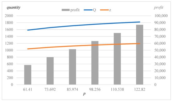
Figure 4.
The results for various selling prices .
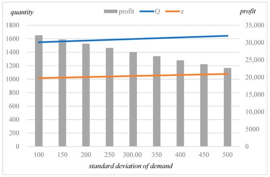
Figure 5.
The results for various standard deviations of demand .
5.3. Analysis of Changes along Product Lifecycle
A remanufactured product follows the standard lifecycle pattern of a new product, with five stages: introduction, growth, maturity, decline, and end-of-life. However, these stages lag compared with their corresponding stages for a new product in time [58]. In the remainder of this section, we refer to the stages of the lifecycle of a remanufactured product. The data shown in Table 6 are from the survey of ReCellular in Mutha, Bansal, and Guide [12].
Table 6.
The data from ReCellular along the lifecycle in Mutha, Bansal, and Guide [12].
As shown in Table 7 and Figure 6, the expected profit for the remanufacturer increases from the introduction to the growth stage, and decreases from the growth stage to the end-of-life. On the one hand, profits in the introduction stage are the lowest because of the low quality of cores, where the lowest rating is as high as 80%. This is mainly due to defective products among the new products. The profit during the growth stage is the highest, mainly because the quality of cores is better than in the introduction stage, the selling price is higher, and the rate of change in demand is lower than in the mature, decline, and end-of-life stages. The decline in profits from the growth stage to the decline stage occurs because the selling price decreases and the standard deviation of demand increases.
Table 7.
The results along the lifecycle.
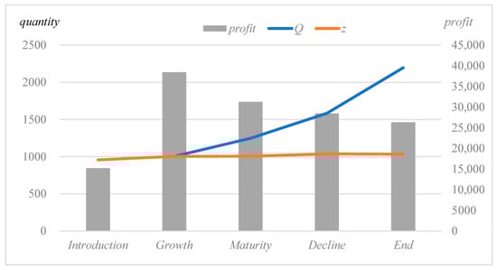
Figure 6.
The results along the lifecycle.
On the other hand, the quantity of acquisition increases with the lifecycle, whereas the quantity of production remains stable. The rate of utilization of cores decreases and the cores are fully utilized in the introduction and growth stages at a high selling price.
The most profitable stage is the growth stage, mainly because the product is well recognized by customers in the growth stage and its price is relatively high. Therefore, remanufacturers should seize business opportunities in the early stage rather than the late stage of the product’s lifecycle.
6. Conclusions and Proposals for Further Research
In this study, we considered the optimal acquisition of products with a high monetary value, e.g., electronic products, by a third-party remanufacturer. The 3PRs acquire used products of unknown quality and sort them into different grades. We developed models to determine the acquisition and quantity of production for the remanufacturer. The optimal models of acquisition and production under deterministic and stochastic demands were established, and the corresponding analytically tractable solutions to them were given. The proposed models were further verified and visualized through numerical work. We also analyzed the trend of changes in the remanufacturer’s profit, the quantity of acquisition, and rate of utilization of cores from the perspective of the entire lifecycle. The results show that the optimal production quantity does not decrease in acquisition quantity, the rate of utilization of the recycled parts increases when the acquisition cost decreases, and the optimal quantity of acquisition/production and the minimum expected profit increases when the selling price increases and decreases when the uncertainty of demand and acquisition cost increases. The practical management implications of this study are as follows. First, we provided analytically tractable solutions for the acquisition and production problem when the used products purchased are unsorted, which will give accurate quantitative guidance to the acquisition and production decisions of remanufacturing enterprises. Second, we analyzed the influence of relevant factors on the acquisition quantity, remanufacturing quantity, and enterprises profits, which will provide qualitative guidance for the remanufacturing enterprises to weigh various factors. Third, the results noted that remanufacturers should pay more attention to remanufacturing activities early in the life of products.
Some interesting avenues for future research emerge from this work, as the same methods and similar models can be used to explore other combinatorial optimization problems—for example, piecewise-linear, unsplittable, and multi-commodity flow problems, and network design and routing problems. This study also offers several interesting directions for future research. First, we built a single-period model to optimize the acquisition of products with a short lifecycle. A multi-period model for optimizing the acquisition of products with a long lifecycle should be built in future research. Second, we ignored the cost structure and simply considered a linearly variable cost of acquisition. Verifying this assumption is an interesting challenge for future research [28]. Third, we explored the policy of the acquisition of unsorted cores and the quantity-dependent piecewise costs of production from the perspective of third-party remanufacturers. This can be extended from the perspective of the supply chain in future work.
Author Contributions
H.S.: conceptualization, methodology, software, data curation, writing (original draft), visualization, formal analysis, investigation, and writing. Y.L.: conceptualization, methodology, and writing—review and editing. All authors have read and agreed to the published version of the manuscript.
Funding
This research was funded by the National Natural Science Foundation of China [grant number 72102126]; the Shandong Provincial Natural Science Foundation, China [grant number ZR2021QG037]; and Humanities and Social Sciences Foundation of the Ministry of Education of China [grant number 21YJC630119].
Data Availability Statement
In this paper, no real data are used.
Conflicts of Interest
The authors declare no conflict of interest.
Appendix A
Proof of Lemma 1.
- a.
- On the one hand, is continuous when , for , where and . Similarly, is always continuous when , for , where and . Therefore, is continuous.On the other hand, let and denote the production costs when the production quantities are and , respectively. We assume that and , where for .The difference between and can be expressed asIf , then .If , thenNow, we demonstrated that is increasingly continuous. In addition, with the assumption that a lower-quality grade is more expensive to convert to a finished unit, , so is a piecewise-linear convex function and increasingly continuous in the interval for a given .
- b.
- Case 1: For a fixed the production quantity , let and denote the production cost when the acquisition quantities are and , respectively. We assume that when the acquisition quantity is and when the acquisition quantity is , where for .Therefore, the difference between and can be expressed asIf , thenIf , thenTherefore, is always negative when .Case 2: For a fixed cost, the production quantity ,, and , which is explores in the final sections.Therefore, is always negative when .Previously, we demonstrated that is non-increasing in for a given production quantity . □
Proof of Lemma 2.
Given an acquisition quantity , is in the interval, i.e., . Similarly, suppose is in the interval when the acquisition quantity is , . It is evident that , and the larger is, the smaller and are. The total cost function can be expressed as follows, respectively:
The first difference in the total cost is the following expression:
Particularly if , the first difference is .
Since is a monotonically increasing (non-decreasing) function of . We conclude by noting that, since , has a unique minimum. □
Proof of Proposition 3.
Case 1. Suppose that , where . Since and maximizes the function, so .
In addition, by definitions of , .
Therefore, the optimal production quantity is if for .
Case 2. Suppose that , where . Given that the function monotonically increases in and , we have , , , , and .
Therefore, the optimal production quantity is if for . □
Proof of Lemma 3.
The optimal production quantity is when the acquisition quantity is great enough , then , , so the first difference in is always negative when , i.e., . So, is the maximum possible acquisition quantity.
Therefore, according to Proposition 3, when the acquisition quantity gradually increases from 0 to , the corresponding optimal production quantity is and , successively. □
Proof of Lemma 4.
The objective function is a piecewise function, and it is differentiable on each piece. Combining with Proposition 3, we should prove that the first difference in is non-increasing in in the intervals when and , when and , and when , and is also non-increasing at the inflection point when and and when and .
First, if , the optimal production quantity is , and the first difference in in is , which decreases in . Second, if , the optimal production quantity is , and the first difference in in is , which is constant. Third, if , the optimal production quantity is , and the first difference in in is , which decreases in . In conclusion, , which does not increase in .
Next, let , , , and , then and are the inflection points.
For , so . Consequently,
Thus, we demonstrated that the first difference in does not increase in . □
References
- Singhal, D.; Tripathy, S.; Jena, S.K. Remanufacturing for the circular economy: Study and evaluation of critical factors. Resour. Conserv. Recycl. 2020, 156, 104681. [Google Scholar] [CrossRef]
- Gong, Q.; Xiong, Y.; Jiang, Z.; Zhang, X.; Hu, M.; Cao, Z. Economic, environmental and social benefits analysis of remanufacturing strategies for used products. Mathematics 2022, 10, 3929. [Google Scholar] [CrossRef]
- Liu, Z.; Li, K.W.; Tang, J.; Gong, B.; Huang, J. Optimal operations of a closed-loop supply chain under a dual regulation. Int. J. Prod. Econ. 2021, 233, 107991. [Google Scholar] [CrossRef]
- Guide, V.D.R. Production planning and control for remanufacturing: Industry practice and research needs. J. Oper. Manag. 2000, 18, 467–483. [Google Scholar] [CrossRef]
- Guide, V.D.R.; Van Wassenhove, L.N. Managing product returns for remanufacturing. Prod. Oper. Manag. 2001, 10, 142–155. [Google Scholar] [CrossRef]
- Sun, H.; Chen, W.; Liu, B.; Chen, X. Economic lot scheduling problem in a remanufacturing system with returns at different quality grades. J. Clean. Prod. 2018, 170, 559–569. [Google Scholar] [CrossRef]
- Wei, S.; Tang, O.; Sundin, E. Core (product) acquisition management for remanufacturing: A review. J. Remanuf. 2015, 5, 4. [Google Scholar] [CrossRef]
- Sun, H.; Chen, W.; Ren, Z.; Liu, B. Optimal policy in a hybrid manufacturing/remanufacturing system with financial hedging. Int. J. Prod. Res. 2017, 55, 5728–5742. [Google Scholar] [CrossRef]
- Teunter, R.H.; Flapper, S.D.P. Optimal core acquisition and remanufacturing policies under uncertain core quality fractions. Eur. J. Oper. Res. 2011, 210, 241–248. [Google Scholar] [CrossRef]
- Bulmuş, S.C.; Zhu, S.X.; Teunter, R.H. Optimal core acquisition and pricing strategies for hybrid manufacturing and remanufacturing systems. Int. J. Prod. Res. 2014, 52, 6627–6641. [Google Scholar] [CrossRef]
- Chen, Y.; Li, B.; Zhang, G.; Bai, Q. Quantity and collection decisions of the remanufacturing enterprise under both the take-back and carbon emission capacity regulations. Transport Res. E-LOG 2020, 141, 102032. [Google Scholar] [CrossRef]
- Mutha, A.; Bansal, S.; Guide, V.D.R. Managing demand uncertainty through core acquisition in remanufacturing. Prod. Oper. Manag. 2016, 25, 1449–1464. [Google Scholar] [CrossRef]
- Mukhopadhyay, S.K.; Ma, H. Joint procurement and production decisions in remanufacturing under quality and demand uncertainty. Int. J. Prod. Econ. 2009, 120, 5–17. [Google Scholar] [CrossRef]
- Ferguson, M.; Guide, V.D.R.; Koca, E.; Souza, G.C. The value of quality grading in remanufacturing. Prod. Oper. Manag. 2009, 18, 300–314. [Google Scholar] [CrossRef]
- Mutha, A.; Bansal, S.; Guide, V.D.R. Selling assortments of used products to Third-Party Remanufacturers. Prod. Oper. Manag. 2019, 28, 1792–1817. [Google Scholar] [CrossRef]
- Galbreth, M.R.; Blackburn, J.D. Optimal acquisition and sorting policies for remanufacturing. Prod. Oper. Manag. 2006, 15, 384–392. [Google Scholar] [CrossRef]
- Galbreth, M.R.; Blackburn, J.D. Optimal acquisition quantities in remanufacturing with condition uncertainty. Prod. Oper. Manag. 2010, 19, 61–69. [Google Scholar] [CrossRef]
- Zikopoulos, C.; Tagaras, G. Impact of uncertainty in the quality of returns on the profitability of a single-period refurbishing operation. Eur. J. Oper. Res. 2007, 182, 205–225. [Google Scholar] [CrossRef]
- Zikopoulos, C.; Tagaras, G. On the attractiveness of sorting before disassembly in remanufacturing. IIE Trans. 2008, 40, 313–323. [Google Scholar] [CrossRef]
- Ngueveu, S.U. Piecewise linear bounding of univariate nonlinear functions and resulting mixed integer linear programming-based solution methods. Eur. J. Oper. Res. 2019, 275, 1058–1071. [Google Scholar] [CrossRef]
- Fortz, B.; Gouveia, L.; Joyce-Moniz, M. Models for the piecewise linear unsplittable multicommodity flow problems. Eur. J. Oper. Res. 2017, 261, 30–42. [Google Scholar] [CrossRef]
- Fortz, B.; Gorgone, E.; Papadimitriou, D. A Lagrangian heuristic algorithm for the time-dependent combined network design and routing problem. Networks 2017, 69, 110–123. [Google Scholar] [CrossRef]
- Atasu, A.; Guide, V.D.R.; Van Wassenhove, L.N. Product Reuse Economics in Closed-Loop Supply Chain Research. Prod. Oper. Manag. 2008, 17, 483–496. [Google Scholar] [CrossRef]
- Jena, S.K.; Sarmah, S.P. Future aspect of acquisition management in closed-loop supply chain. Int. J. Sustain. Eng. 2016, 9, 266–276. [Google Scholar] [CrossRef]
- Peng, H.; Shen, N.; Liao, H.; Xue, H.; Wang, Q. Uncertainty factors, methods, and solutions of closed-loop supply chain—A review for current situation and future prospects. J. Clean. Prod. 2020, 254, 120032. [Google Scholar] [CrossRef]
- Xing, S.; Jiang, Z.; Zhang, X.; Wang, Y. Product design sheme generation and optimization decisions while considering remanufacturability. Mathematics 2022, 10, 2477. [Google Scholar] [CrossRef]
- Liu, Z.; Li, K.W.; Li, B.-Y.; Huang, J.; Tang, J. Impact of product-design strategies on the operations of a closed-loop supply chain. Transport Res. E-LOG 2019, 124, 75–91. [Google Scholar] [CrossRef]
- Atasu, A.; Toktay, L.B.; Van Wassenhove, L.N. How collection cost structure drives a manufacturer’s reverse channel choice. Prod. Oper. Manag. 2013, 22, 1089–1102. [Google Scholar] [CrossRef]
- Wang, L.; Cai, G.G.; Tsay, A.A.; Vakharia, A.J. Design of the reverse channel for remanufacturing: Must profit-maximization harm the environment? Prod. Oper. Manag. 2017, 26, 1585–1603. [Google Scholar] [CrossRef]
- Shi, T.; Chhajed, D.; Wan, Z.; Liu, Y. Distribution channel choice and divisional conflict in remanufacturing operations. Prod. Oper. Manag. 2020, 29, 1702–1719. [Google Scholar] [CrossRef]
- Qiang, Q.; Ke, K.; Anderson, T.; Dong, J. The closed-loop supply chain network with competition, distribution channel investment, and uncertainties. Omega 2013, 41, 186–194. [Google Scholar] [CrossRef]
- Sahebi, H.; Ranjbar, S.; Teymouri, A. Investigating different reverse channels in a closed-loop supply chain: A power perspective. Oper. Res. 2022, 22, 1939–1985. [Google Scholar] [CrossRef]
- Yang, C.-H.; Ma, X.; Talluri, S. Optimal acquisition decision in a remanufacturing system with partial random yield information. Int. J. Prod. Res. 2018, 57, 1624–1644. [Google Scholar] [CrossRef]
- Yang, C.-H.; Wang, J.; Ji, P. Optimal acquisition policy in remanufacturing under general core quality distributions. Int. J. Prod. Res. 2014, 53, 1425–1438. [Google Scholar] [CrossRef]
- Tao, F.; Fan, T.; Jia, X.; Lai, K.K. Optimal production strategy for a manufacturing and remanufacturing system with return policy. Oper. Res. 2021, 21, 251–271. [Google Scholar] [CrossRef]
- Matsui, K. Optimal timing of acquisition price announcement for used products in a dual-recycling channel reverse supply chain. Eur. J. Oper. Res. 2022, 300, 615–632. [Google Scholar] [CrossRef]
- Li, K.; Liu, J.; Fu, H.; Liu, B. Acquisition and pricing strategies in hybrid manufacturing-remanufacturing systems. J. Manuf. Syst. 2020, 57, 217–230. [Google Scholar] [CrossRef]
- Guide, V.D.R.; Teunter, R.H.; Van Wassenhove, L.N. Matching demand and supply to maximize profits from remanufacturing. Manuf. Serv. Oper. Manag. 2003, 5, 303–316. [Google Scholar] [CrossRef]
- Zhang, X.-M.; Li, Q.-W.; Liu, Z.; Chang, C.-T. Optimal pricing and remanufacturing mode in a closed-loop supply chain of WEEE under government fund policy. Comput. Ind. Eng. 2021, 151, 106951. [Google Scholar] [CrossRef]
- Dominguez, R.; Cannella, S.; Ponte, B.; Framinan, J.M. On the dynamics of closed-loop supply chains under remanufacturing lead time variability. Omega 2020, 97, 102106. [Google Scholar] [CrossRef]
- Schulz, T.; Voigt, G. A flexibly structured lot sizing heuristic for a static remanufacturing system. Omega 2014, 44, 21–31. [Google Scholar] [CrossRef]
- Hong, X.; Cao, X.; Gong, Y.; Chen, W. Quality information acquisition and disclosure with green manufacturing in a closed-loop supply chain. Int. J. Prod. Econ. 2021, 232, 107997. [Google Scholar] [CrossRef]
- Hahler, S.; Fleischmann, M. Strategic grading in the product acquisition process of a reverse supply chain. Prod. Oper. Manag. 2017, 26, 1498–1511. [Google Scholar] [CrossRef]
- Yanıkoğlu, İ.; Denizel, M. The value of quality grading in remanufacturing under quality level uncertainty. Int. J. Prod. Res. 2020, 59, 839–859. [Google Scholar] [CrossRef]
- Radhi, M.; Zhang, G. Optimal configuration of remanufacturing supply network with return quality decision. Int. J. Prod. Res. 2015, 54, 1487–1502. [Google Scholar] [CrossRef]
- Üster, H.; Hwang, S.O. Closed-Loop supply chain network design under demand and return uncertainty. Transport. Sci. 2017, 51, 1063–1085. [Google Scholar] [CrossRef]
- Piñeyro, P.; Viera, O. The economic lot-sizing problem with remanufacturing and heterogeneous returns: Formulations, analysis and algorithms. Int. J. Prod. Res. 2021, 60, 3521–3533. [Google Scholar] [CrossRef]
- Zhou, S.X.; Tao, Z.; Chao, X. Optimal control of inventory systems with multiple types of remanufacturable products. Manuf. Serv. Oper. Manag. 2011, 13, 20–34. [Google Scholar] [CrossRef]
- Ponte, B.; Cannella, S.; Dominguez, R.; Naim, M.M.; Syntetos, A.A. Quality grading of returns and the dynamics of remanufacturing. Int. J. Prod. Econ. 2021, 236, 108129. [Google Scholar] [CrossRef]
- Karlin, S. Dynamic inventory policy with varying stochastic demands. Manag. Sci. 1960, 6, 231–258. [Google Scholar] [CrossRef]
- Lu, Y.; Song, M. Inventory control with a fixed cost and a piecewise linear convex cost. Prod. Oper. Manage. 2014, 23, 1966–1984. [Google Scholar] [CrossRef]
- Caliskan-Demirag, O.; Chen, O.F.; Yang, Y. Ordering policies for periodic-review inventory systems with quantity-dependent fixed costs. Oper. Res. 2012, 60, 785–796. [Google Scholar] [CrossRef]
- Li, Q.; Wu, X.; Cheung, K.L. Optimal policies for inventory systems with separate delivery-request and order-quantity decisions. Oper. Res. 2009, 57, 626–636. [Google Scholar] [CrossRef]
- Sillanpää, V.; Liesiö, J.; Käki, A. Procurement decisions over multiple periods under piecewise-linear shortage costs and fixed capacity commitments. Omega 2021, 100, 102207. [Google Scholar] [CrossRef]
- Ardestani-Jaafari, A.; Delage, E. Robust optimization of sums of piecewise linear functions with application to inventory problems. Oper. Res. 2016, 64, 474–494. [Google Scholar] [CrossRef]
- Lu, Y.; Song, M.; Yang, Y. Approximation approaches for inventory systems with general production/ordering cost structures. Prod. Oper. Manag. 2018, 27, 417–432. [Google Scholar] [CrossRef]
- Evans, D.L.; Leemis, L.M.; Drew, J.H. The distribution of order statistics for discrete random variables with applications to bootstrapping. INFORMS J. Comput. 2006, 18, 19–30. [Google Scholar] [CrossRef]
- Krikke, H.; Hofenk, D.; Wang, Y. Revealing an invisible giant: A comprehensive survey into return practices within original (closed-loop) supply chains. Resour. Conserv. Recycl. 2013, 73, 239–250. [Google Scholar] [CrossRef]
Disclaimer/Publisher’s Note: The statements, opinions and data contained in all publications are solely those of the individual author(s) and contributor(s) and not of MDPI and/or the editor(s). MDPI and/or the editor(s) disclaim responsibility for any injury to people or property resulting from any ideas, methods, instructions or products referred to in the content. |
© 2023 by the authors. Licensee MDPI, Basel, Switzerland. This article is an open access article distributed under the terms and conditions of the Creative Commons Attribution (CC BY) license (https://creativecommons.org/licenses/by/4.0/).