Resonance Analysis of Horizontal Nonlinear Vibrations of Roll Systems for Cold Rolling Mills under Double-Frequency Excitations

Abstract

In this paper, the fractional order differential terms are introduced into a horizontal nonlinear dynamics model of a cold mill roller system. The resonance characteristics of the roller system under high-frequency and low-frequency excitation signals are investigated. Firstly, the dynamical equation of the roller system with a fractional order is established by replacing the normal damping term with a fractional damping term. Secondly, the fast-slow variable separation method is introduced to solve the dynamical equation. The amplitude frequency response characteristics of the system are analyzed. The study finds that there are three equilibrium points. The characteristics of the three equilibrium points and the critical forces causing the bifurcation are investigated. Due to the different orders of the fractional derivatives, various new resonant phenomena are found in the systems with single-well and double-well potentials. Additionally, the double resonance occurs while p = 0.3 or 1.0, and single resonance occurs while p = 1.8. Unlike integer order systems, the critical resonance amplitude of high-frequency signals in fractional order systems depends on the damping strength and is influenced by the fractional order damping. This study provides a broader picture of the vibration characteristics of the roll system for rolling mills.

1. Introduction

The vibration of the roll system during the rolling process not only affects the stable operation of the equipment, but may also cause vibration patterns on the surface of the strip and can also restrict the product quality [1]. Early studies on roller vibration mostly consider the phenomenon to be a linear steady-state system [2]. However, in fact, there are many nonlinear factors in the operation of the roll system, such as nonlinear damping and nonlinear stiffness. Currently, most scholars have studied the linear and nonlinear aspects of roll system vibration by treating the roll system as a general integer order system. Hou D.X. studied the vertical–horizontal coupling vibration characteristics of strip mill rolls [3,4,5,6]. Huang J.L. investigated the effect of asymmetric structural parameters on mill stability and also investigated the effect of asymmetric friction coefficients on vibration and stability in hot rolling mills [7,8]. Sun Y.Y. investigated the nonlinear vibration characteristics of the rolling mill system by considering the rolling interface roughness [9]. He D.P. analyzed the non-linear vertical vibration characteristics of a corrugated roll mill roll system under parametric excitation [10,11,12]. Liu B. studied the nonlinear vibration characteristics of strip mills under the action of roll–roll coupling [13,14]. Zhang R.C. investigated the parametric excitation of horizontal nonlinear vibrations in a single-roll drive mill roll system [15]. Yang X. studied the vertical nonlinear vibration model of the cold rolling mill roll system and analyzed the system stability [16].

However, it has been found that integer order differential equations deviate significantly from theoretical and experimental results when modelling practical problems. In fact, fractional derivatives are very useful for describing the viscoelastic properties of materials or the dissipative forces of structural dynamics in engineering practice [17,18]. This is because fractional models can deliver a more accurate description of engineering systems and provide more insight into the intrinsic properties of current physical systems [19,20,21,22,23,24,25,26,27]. An improved fractional order DE algorithm is proposed in this study to improve the efficiency of achieving the optimal strategy of a real-time underwater countermeasure. Additionally, the order of a fractional order DE can affect the convergence rate and optimization error, which can also be tuned to satisfy different underwater requirements [28]. A novel nonlinear vibration isolator in the shape of a circular ring is investigated. When the ring is compressed along a diametral line, it exhibits highly nonlinear geometric stiffness due to the effects of stretching-induced tension coupled with the curvature changes [29]. A magnetic field coupling fractional step lattice Boltzmann model can be utilized for the complex interfacial behavior in magnetic multiphase flows [30]. As a result, fractional numbers are used in a wide range of scientific and engineering applications, such as viscoelastic material models [31,32], fluid mechanics [33,34,35], control [36,37], bioengineering [38], and mechanics [39,40]. The introduction of fractional theory into the dynamic properties of roller systems can greatly improve these deficiencies. Moreover, the fractional differential term possesses not only damping properties, but also stiffness properties in modeling dynamical problems [41,42]. In this paper, a richer dynamic characteristic of the mill roll system is obtained through theoretical analysis and simulation, while the relationship between the influence of system parameters on the vibration resonance of the roll system is investigated.

The structure of this article is as follows: Section 2 introduces the fractional differential term into the roller dynamic characteristics that are under a two frequency excitation. Section 3 uses the fast-slow variable separation method to obtain an approximate analytical solution of the vibration system of the roll system and the response amplitude gain Q. Additionally, the bifurcation and vibration resonance is also discussed in that section. In Section 4, the influence of each parameter on the vibration resonance of single-well and double-well system, respectively, are discussed. Lastly, in Section 5, the conclusions of this paper are presented.

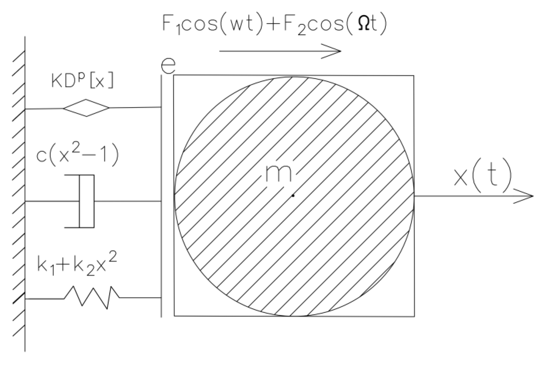
2. Horizontal Nonlinear Equation of the Roller System

The roller system has nonlinear characteristics during the rolling process. By referencing the model of the roller system [43] and by introducing the duffing oscillator model, we can establish the horizontal nonlinear parameter vibration model of the roller system with the fractional order, as is shown in Figure 1. According to the vibration model in Figure 1, the horizontal nonlinear kinematic equation of the roll system can be established as per the following:

$$m\ddot{x}(t)+c(x^2(t)-1)\dot{x}(t)+(k_1+k_2{x}^2(t))x(t)+K{D}^p[x(t)]=F_1\cos (\omega t)+F_2\cos (\Omega t),(0<p<2)$$

(1)

where K is the fractional differential term coefficient and K > 0, p is the fractional differential term order. Further, c is the nonlinear damping coefficient, k₁ is the linear stiffness coefficient, k₂ is the nonlinear stiffness coefficient, m is equivalent mass of the roll, F₁ is the low-frequency excitation amplitude, F₂ is the high-frequency excitation amplitudes, ω is the low excitation frequency, Ω is the high excitation frequency, e is the clearance between the bearing housing and the frame, and x(t) is the horizontal displacement of the roller system. Due to the presence of e, the roll system vibrates back and forth under horizontal excitation forces, which is defined as a horizontal excitation force of $F_1\cos (\omega t)+F_2\cos (\Omega t)$.

In order to better describe the intrinsic relationships of engineering materials, the ordinary damping term is replaced by a fractional damping term, thus introducing the following variable substitution:

$$\delta =c/m=K/m, {\omega }_0=\sqrt{k_1/m}, \beta =k_2/m,f=F_1/m, F=F_2/m$$

(2)

Then, the vibration equation of the horizontal nonlinear system of Equation (1) can be written as per the following:

$$\ddot{x}(t)+{\omega }_0^{2}x(t)+\delta D^p[x(t)]+\beta x^3(t)=f\cos (\omega t)+F\cos (\Omega t),(0<p<2)$$

(3)

It is assumed here that $\delta >0,f<<1,\Omega >>\omega$ and the system have different vibrational properties when the value of the fractional order p is between (0,1] and (1,2), and when the potential energy function of the system is the following:

$$V(x)={\omega }_0^2{x}^2\mathrm{/2}+\beta x^4\mathrm{/4}$$

(4)

There is no unique form of definition for fractional order derivatives, and different types of definitions of fractional order derivatives are derived depending on the context of the study. There are three usual definitions that are used, namely the Riemann–Liouville (R–L) definition, the Grünwald–Letnikov (G–L) definition, and the Caputo definition. In the system defined by Equation (3), the roll system displacements are first order continuously differentiable in [0, T] and the roll system accelerations are integrable in [0, T]. Therefore, for each order p (0 < p < 2), both the Riemann–Liouville and Grünwald–Letnikov derivatives exist and they are equivalent. However, the R–L approach leads to the initial conditions containing limiting values for the fractional derivatives of t = t₀, which do not have a known physical meaning, thereby making the results problematic in terms of practical applications in the village. Therefore, this paper adopts a more engineeringly meaningful definition of Caputo in order to deal with fractional order differential terms.

For a given function x(t), $t\in (t_0,t_x)$ is the fractional order of the Caputo definition, as per [44].

$${}_C{D}_{t_0,t}^p[x(t)]=\frac{1}{\Gamma (m-p)}{\displaystyle {\int }_{t_0}^t\frac{x^{(m)}(\tau )}{{(t-\tau )}^{1+p-m}}}d\tau$$

(5)

where m = [p] is an integer, [] means to take an integer, and Γ(z) is the Gamma function, thus satisfying Γ(z + 1) = z Γ(z).

When p = 1, there are no fractional differential terms present. Suppose t₀ = 0 and t = t_i for the different values of p, then the derivative under the Caputo definition is as per [45].

When 0 < p < 1:

$$\begin{array}{l}[{}_{C}D_{t_0,t}^{p}x(t){]}_{t=t_i}=\frac{1}{\Gamma (1-\alpha )}{\displaystyle {\int }_{t_0}^{t_i}\frac{\dot{x}(\tau )}{{(t_i-\tau )}^{\alpha }}}d\tau \\ =\frac{1}{\Gamma (1-p)}{\displaystyle \sum _{k=0}^{i-1}{\displaystyle {\int }_{t_k}^{t_{k+1}}\frac{\dot{x}(\tau )}{{(t_i-\tau )}^p}}d\tau }\\ \approx \frac{1}{\Gamma (1-\alpha )}{\displaystyle \sum _{k=0}^{i-1}{\displaystyle {\int }_{t_k}^{t_{k+1}}\frac{\text{1}}{{(t_i-\tau )}^p}\frac{x(t_{k+1})-x(t_k)}{\Delta t}}d\tau }\\ ={\displaystyle \sum _{k=0}^{i-1}\frac{\Delta t^{-p}}{\Gamma (2-\alpha )}[{(i-k)}^{1-p}-{(i-k-1)}^{1-p}](x(t_{k+1})-x(t_k))}\end{array}$$

(6a)

when 1 < p < 2:

$$\begin{array}{l}[{}_{C}D_{t_0,t}^{p}x(t){]}_{t=t_i}=\frac{1}{\Gamma (2-n)}{\displaystyle {\int }_{t_0}^{t_i}\frac{\ddot{x}(\tau )}{{(t_i-\tau )}^{1-p}}d\tau }\\ =\frac{1}{\Gamma (2-p)}{\displaystyle \sum _{k=0}^{i-1}{\displaystyle {\int }_{t_k}^{t_{k+1}}\frac{\ddot{x}(\tau )}{{(t_i-\tau )}^{1-p}}}d\tau }\\ \approx \frac{1}{\Gamma (2-p)}{\displaystyle \sum _{k=0}^{i-1}{\displaystyle {\int }_{t_k}^{t_{k+1}}\frac{1}{{(t_i-\tau )}^{1-p}}\frac{\dot{x}(t_{k+1})-\dot{x}(t_k)}{\Delta t}}d\tau }\\ =\frac{1}{\Gamma (2-p)}\frac{x(t_{i-k-1})-2x(t_{i-k})+x(t_{i-k+1})}{\Delta t^2}{\displaystyle {\int }_{t_k}^{t_{k+1}}{\tau }^{1-p}d\tau }\end{array}$$

(6b)

Thus the rewritten Equation (3) is as follows:

$$\{\begin{array}{l}\dot{x}=y\\ \dot{y}=-{\omega }_0^{2}x-\beta x^3-\delta \frac{d^{p}x}{d{t}^p}+f_1\cos (\omega t)+f_2\cos (\Omega t)\end{array}$$

(7)

The discrete form is as follows:

$$\{\begin{array}{l}{x}_i=x_{i-1}+y_{i-1}\Delta t\\ y_i=y_{i-1}+[-{\omega }_0^2{x}_{i-1}-\beta x_{i-1}^3-\delta \frac{d{x}_{i-1}^p}{d{t}^p}+(f_1{)}_{i-1}+(f_2{)}_{i-1}]\Delta t\end{array}$$

(8)

The above formula is the algorithm for finding the fractional differential terms under the Caputo definition. Numerous studies have shown that the fractional order differential theory defined by Caputo above is accurate and is also reliable for solving the dynamic properties of nonlinear systems [46,47,48,49,50].

3. Bifurcation and Vibration Resonance

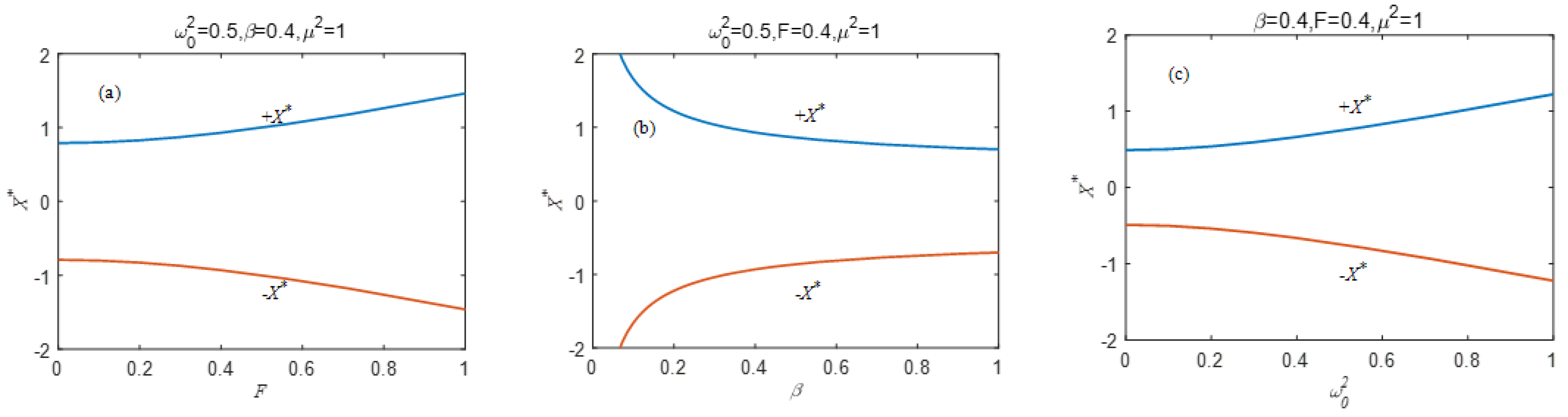
3.1. Pitchfork Bifurcation

Due to the different orders of the fractional derivatives, various new resonance phenomena are found for single-well and double-well systems, respectively. Furthermore, the value of the fractional order can be used as a bifurcation parameter by which the response characteristics of the mill roll system can be analyzed.

In the roller vibration system, the fast and slow variable separation method can be used to analyze the response characteristics of the system under the dual frequency signal excitation; it can also be used to eliminate the fast variables in the system. When compared with the averaging and multi-scale methods, this method can obtain a stable solution of the system and can effectively avoid the jump phenomenon in the response of a non-linear system.

According to the fast and slow variable separation method, assume $x=\mathrm{X}(t)+\mathsf{\Psi }(t,\Omega t)$. Where X(t) is a slow variable with the period of $2\pi /\omega$, and $\mathsf{\Psi }(t,\Omega t)$ is a fast variable with the period of $2\pi /\Omega$, then evidently the following applies:

$$\langle \mathsf{\Psi }(t,\Omega )\rangle =\frac{\Omega }{2\pi }{\displaystyle {\int }_0^{2\pi }\mathsf{\Psi }(t,\Omega )}dt=0$$

(9)

Substitute $x=\mathrm{X}(t)+\mathsf{\Psi }(t,\Omega t)$ into Equation (3) and separate fast and slow variables

$$\frac{d^2\mathsf{\Psi }}{d{t}^2}+\delta \frac{d^p\mathsf{\Psi }}{d{t}^p}=-({\omega }_0^2+3\beta {\mathrm{X}}^2)(\mathsf{\Psi }-\langle \mathsf{\Psi }\rangle )-3\beta \mathrm{X}({\mathsf{\Psi }}^2-\langle {\mathsf{\Psi }}^2\rangle )-\beta ({\mathsf{\Psi }}^3-\langle {\mathsf{\Psi }}^3\rangle )+F\cos (\Omega t)$$

(10a)

$$\frac{d^2\mathrm{X}}{d{t}^2}+\delta \frac{d^p\mathrm{X}}{d{t}^p}=-{\omega }_0^2\langle \mathsf{\Psi }\rangle -\beta {\langle \mathsf{\Psi }\rangle }^3-({\omega }_0^2+3\beta \langle {\mathsf{\Psi }}^2\rangle )\mathrm{X}-3\beta \langle \mathsf{\Psi }\rangle {\mathrm{X}}^2-\beta {\mathrm{X}}^3+f\cos (\omega t)$$

(10b)

Since $\mathsf{\Psi }$ is the fast variable, $d^2\mathsf{\Psi }/d{t}^2,d^p\mathsf{\Psi }/d{t}^p$>>$\mathsf{\Psi },{\mathsf{\Psi }}^2,{\mathsf{\Psi }}^3$. This results in neglecting all the nonlinear terms on the right hand of Equation (10b) and using Equations (9) and (10b), which can be reduced to the linear form:

$$\frac{d^2\mathsf{\Psi }}{d{t}^2}+\delta \frac{d^p\mathsf{\Psi }}{d{t}^p}+{\omega }_0^2\mathsf{\Psi }=F\cos (\Omega t)$$

(11)

Assume the solution of Equation (11) as per the following:

$$\mathsf{\Psi }=(F/\mu )\cos (\Omega t-\theta )$$

(12)

According to Equation (12), we can obtain

$$\begin{array}{l}\mathsf{\Psi }{\mathrm{|}}_{t=0}=(F/\mu )\cos (-\theta )\\ \mathsf{\Psi }{\mathrm{|}}_{t=\theta /\Omega }=F/\mu \end{array}$$

(13)

According to the fractional derivative formula of the simple harmonic function, we can obtain

$$\frac{d^p\mathsf{\Psi }}{d{t}^p}=\frac{d^p}{d{t}^p}[\frac{F}{\mu }\cos (\Omega t-\theta )]=\frac{F}{\mu }{\Omega }^p\cos (\Omega t-\theta +\frac{p\pi }{2})$$

(14)

which is the use of the method of undetermined coefficients. When substituting Equation (12) into Equation (11), and when calculating and comparing the equation coefficients of $\sin (\Omega t-\theta )$ and $\cos (\Omega t-\theta )$ at both ends of the equation by using triangle male, we can obtain

$$\{\begin{array}{c}-\frac{{\Omega }^{2}F}{\mu }+\delta \frac{{\Omega }^{p}F}{\mu }\cos (\frac{p\pi }{2})+{\omega }_0^2\frac{F}{\mu }=F\cos \theta \\ \delta \frac{{\Omega }^{p}F}{\mu }\sin (\frac{p\pi }{2})=F\sin \theta \end{array}$$

(15)

Then

$${\mu }^2={[{\omega }_0^2+\delta {\Omega }^p\cos (p\pi /2)-{\Omega }^2]}^2+{[\delta {\Omega }^p\sin (p\pi /2)]}^2$$

(16a)

$$\theta =\arctan \frac{\delta {\Omega }^p\sin (p\pi /2)}{{\omega }_0^2+\delta {\Omega }^p\cos (p\pi /2)-{\Omega }^2}$$

(16b)

From Equation (12), one obtains the averaging values of different order of $\mathsf{\Psi }$ within $\left[0,2\pi /\Omega \right]$:

$$\langle \mathsf{\Psi }\rangle =\langle {\mathsf{\Psi }}^3\rangle =0,\langle {\mathsf{\Psi }}^2\rangle =F^2/2{\mu }^2$$

(17)

When one inserts Equations (17) and (12) into Equation (10a), the govern equation for fast motion becomes

$$\frac{d^2\mathrm{X}}{d{t}^2}+\delta \frac{d^p\mathrm{X}}{d{t}^p}+S_1\mathrm{X}+S_2{\mathrm{X}}^3=f\cos (\omega t)$$

(18)

where

$$S_1={\omega }_0^2+3\beta F^2/(2{\mu }^2),S_2=\beta$$

(19)

From Equation (18), we can obtain the potential function of the system:

$$V_e(\mathrm{X})=S_1{\mathrm{X}}^2\mathrm{/2}+S_2{\mathrm{X}}^4\mathrm{/4}$$

(20)

Unlike Equation (4), the $V(x)$, which is completely determined by the parameters ${\omega }_0^2$ and $\beta$, $V_e(X)$, is also affected by the high-frequency excitation force F. When $f=0$, the slow variable system Equation (18) may have three equilibrium points.

$${\mathrm{X}}_1^{\ast }=0,{\mathrm{X}}_2^{\ast }=-\sqrt{-S_1/S_2},{\mathrm{X}}_3^{\ast }=\sqrt{-S_1/S_2}$$

(21)

The slow variable X may behave as the vibration around the stable equilibrium point. From Equation (21), we can know that when the S₁ > 0, then the $V_e$ is a single-well function and that the system has a unique stable equilibrium point $X_1^{*}=0$. When the S₁ < 0, $V_e$ is a double-well function and the system has two stable equilibrium points of ${\mathrm{X}}_{2,3}^{\ast }=\pm \sqrt{-S_1/S_2}$ and one unstable equilibrium point $X_1^{*}=0$. The influence of the system parameters on the equilibrium points are shown in Figure 2. The figures show that the system has a forked bifurcation and that different parameters have different effects on the degree of bifurcation. This phenomenon occurs because the high frequency signal softens the stiffness of the system, as well as alters the equilibrium point of the system, which thus causes the nonlinear system to become a pitchfork bifurcation.

In Equation (19), F is the independent variable. By solving $S_1=0$, we can obtain the critical value that changes the number of equilibrium points in the system, which is the equilibrium point causing the pitchfork bifurcation:

$$F_C=\sqrt{2{\mu }^2\left|{\omega }_0^2\right|/3\beta }$$

(22)

3.2. Vibration Resonance

To obtain the amplitude of the low-frequency excitation, assume $Y=X-X^{*}$ and bring it into Equation (18), thereby eliminating the constant component of the response and retaining the harmonic term as

$$\frac{d^{2}Y}{d{t}^2}+\delta \frac{d^{p}Y}{d{t}^p}+S_{3}Y+S_4{Y}^2+S_5{Y}^3=f\cos (\omega t)$$

(23)

where $S_3={\omega }_r^2=S_1+3S_2{X}^{*2},S_4=3S_2{X}^{*},S_5=\beta$,${\omega }_r$ is the resonance frequency because of $f<<1$. Furthermore, when $t\to \infty$,$\left|Y\right|<<1$, then neglect the nonlinear term in Equation (23) and obtain the linear equation for Y, which is

$$\frac{d^{2}Y}{d{t}^2}+\delta \frac{d^{p}Y}{d{t}^p}+{\omega }_r^{2}Y=f\cos (\omega t)$$

(24)

In using the undetermination coefficient method, we can assume the solution of Equation (24) is $Y=A_L\cos (\omega t-\varphi )$. Therefore, we can insert it into Equation (24), and thus we can obtain

$$A_L=f/\sqrt{{[{\omega }_r^2-{\omega }^2+\delta {\omega }^p\cos (p\pi /2)]}^2+{[\delta {\omega }^p\sin (p\pi /2)]}^2}$$

(25a)

$$\varphi =\arctan \{[\delta {\omega }^p\sin (p\pi /2)]/[{\omega }_r^2-{\omega }^2+\delta {\omega }^p\cos (p\pi /2)]\}$$

(25b)

where $\varphi$ represents the initial distance between the motion and the stable equilibrium point $X^{*}$. This means that $t=0,Y=\cos (\varphi )$ is the initial deviation between $X$ and $X^{*}$. Since p is included in Equation (25b), it has an effect on the value of the initial phase $\varphi$. The initial phase approaches 0 as p approaches 0 or 2. Furthermore, as p varies, $\varphi$ undergoes a solution as the value of p changes from −π/2 to π/2 (or from π/2 to −π/2). As such, the monotonicity of $\varphi$ before the solution is the opposite of the monotonicity after the solution.

The response amplitude is often used to define as $Q=A_L/f$ in order to study the vibrational resonance of the system. This represents the number of times a nonlinear system is amplified by the action of a weak low-frequency signal, thus

$$Q=1/\sqrt{{[{\omega }_r^2-{\omega }^2+\delta {\omega }^p\cos (p\pi /2)]}^2+{[\delta {\omega }^p\sin (p\pi /2)]}^2}$$

(26)

In order to verify the correctness of the analytical solution, an evaluation index of the numerical solution should also be given to quantify the vibration resonance phenomenon of the non-linear system of rolls. The degree of vibration resonance is usually measured by the amplitude gain of the system response to a low frequency input signal. The numerical method calculates the response amplitude as $Q=\sqrt{Q_S^2+Q_C^2}/f$, and where Qs and Qc are the sine and cosine components of the Fourier coefficients [51].

$$Q_S=\frac{2}{pT}{\displaystyle {\int }_0^{pT}x(t)\sin (\omega t)dt,}{Q}_C=\frac{2}{pT}{\displaystyle {\int }_0^{pT}x(t)\cos (\omega t)dt}$$

(27)

where $T=2\pi /\omega$ represents the period of the low-frequency signal and p is a positive integer that should be chosen as large enough to ensure the accuracy of the numerical results. In the theoretical analysis of this paper, only the $2\pi /\omega$ periodic slow variables and $2\pi /\Omega$ periodic sexual fast variables are present. In addition, other higher harmonics are ignored because the amplitudes of other higher harmonics are very small compared to the fundamental frequency when compared to the components.

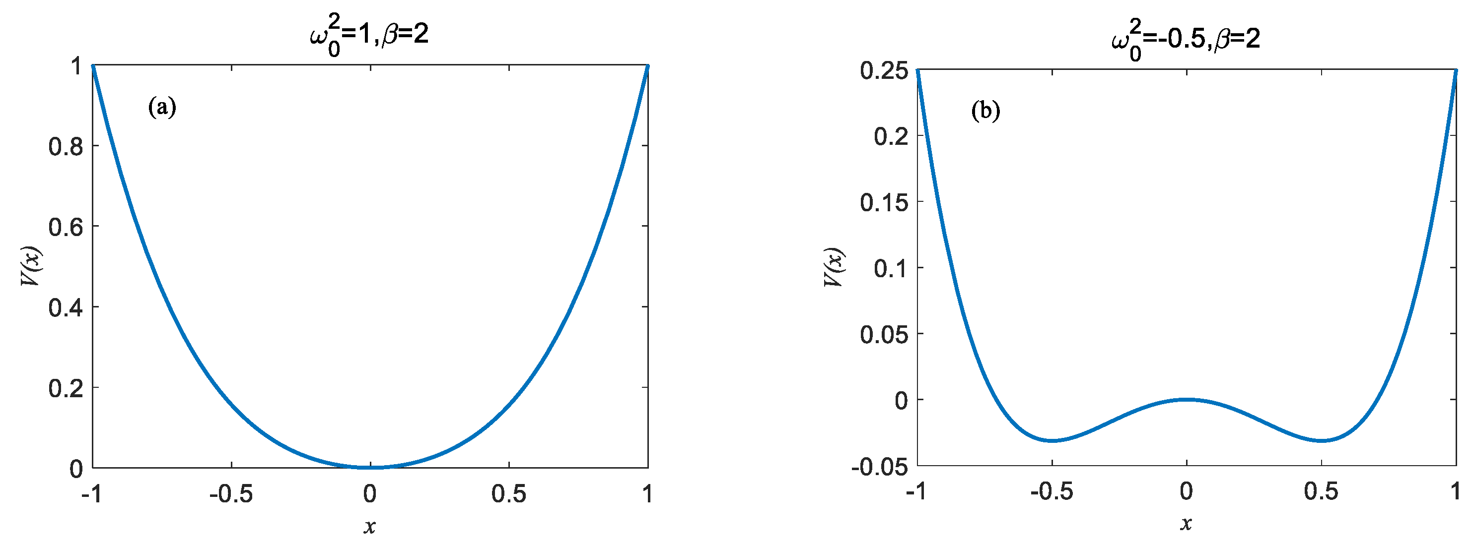
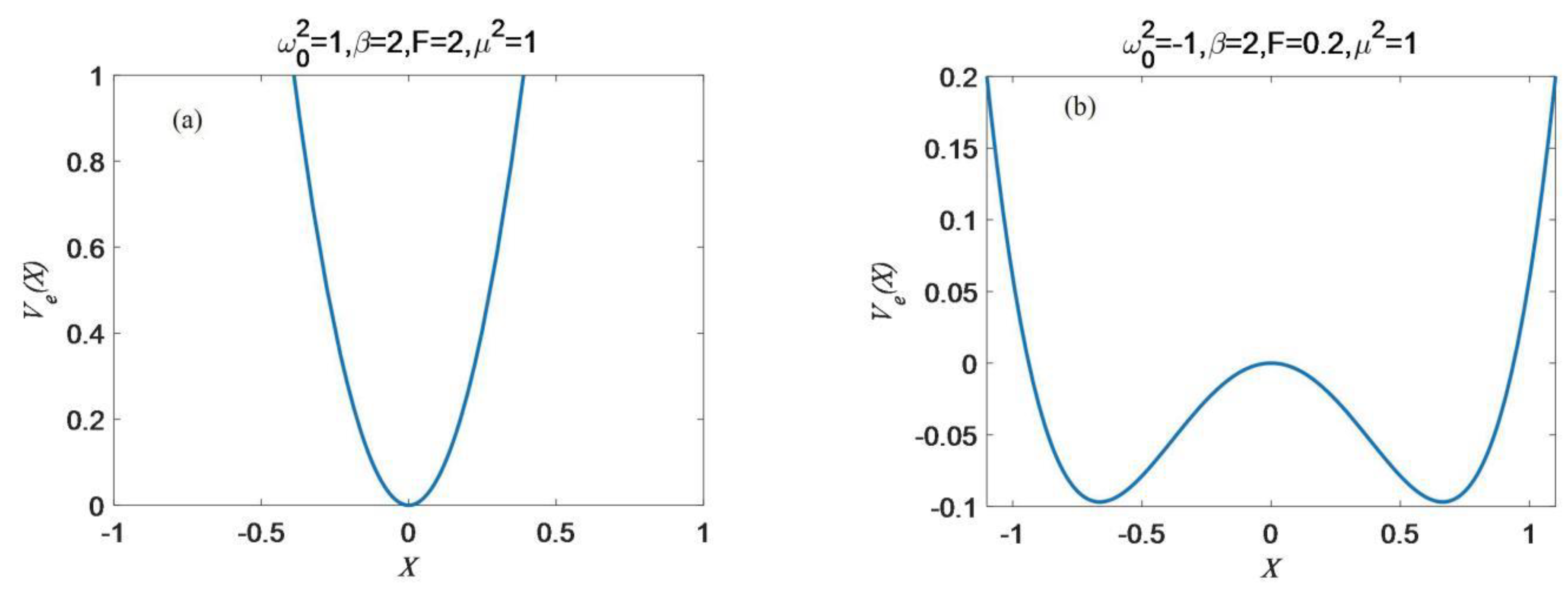
4. Single-well and Double-well Systems

This section studies the single-well and double-well of the roll system described in Equation (3). As shown in Figure 3, the response of the system is limited to within one potential well due to the small amplitude of the externally excited high-frequency signal, which does not allow traversal between two different potential wells. A single-well state is presented. As the external excitation high-frequency signal gradually increases, the response range of the system gradually expands into the other potential well. This results in a double-well phenomenon.

4.1. Single-well System

When ${\omega }_0^2,\beta >0$, $V(x)$ is a single-well potential function (Figure 3a), and it always has $S_1,S_2>0$. $V_e$, then it is also a single well (Figure 4a). Furthermore,$X_1^{*}=0$ is the only stable equilibrium point, thus $S_3=S_1,{\omega }_r=\sqrt{S_3}=\sqrt{S_1}$. As such, let

$$\begin{array}{l}S=[{\omega }_r^2-{\omega }^2+\delta {\omega }^p\cos (p\pi /2){]}^2+[\delta {\omega }^p\sin (p\pi /2){]}^2\\ =[S_3-{\omega }^2+\delta {\omega }^p\cos (p\pi /2){]}^2+[\delta {\omega }^p\sin (p\pi /2){]}^2\\ =[S_1-{\omega }^2+\delta {\omega }^p\cos (p\pi /2){]}^2+[\delta {\omega }^p\sin (p\pi /2){]}^2\\ =[{\omega }_0^2+3\beta F^2/(2{\mu }^2)-{\omega }^2+\delta {\omega }^p\cos (p\pi /2){]}^2+[\delta {\omega }^p\sin (p\pi /2){]}^2\end{array}$$

(28)

As $Q=1/\sqrt{S}$, the system vibration resonance occurs when S takes the minimum value.

Use $\omega$ as a control parameter. When varying the value of $\omega$ and fixing the other parameters, S has a minimum value when the critical frequency ${\omega }_{VR}>0$ is reached, thus making the first part of Equation (28) satisfy $S_{\omega }({\omega }_{VR})=0$. However, it is difficult to obtain an expression for ${\omega }_{VR}$ when $p\ne 1$. By numerical calculation, Figure 5a shows the relationship between ${\omega }_{VR}$ and F and p. The surface is curved and has extreme regions (Figure 5b) in which no resonance occurs. Consider the three different values of p, then the relationship between F and ${\omega }_{VR}$ is shown in Figure 5c and it can be found that the critical frequency increases gradually with the increase in the excitation amplitude F when p ≠ 1. This indicates that the introduction of the fractional differential term has a non-negligible effect on the system. Figure 5d shows the effect of the fractional order on the critical frequency of the system. As can be seen from the figure below, p has a concave curve in the interval [0, 2]. When p = 1, the critical frequency is at the bottom of the valley and increases gradually as p decreases or increases. In Figure 5e, it is clear that a single resonance occurs in the single-well system when the value of p deviates from 1, thereby implying that the new resonance phenomena may be induced as p varies. Figure 5f visually shows the effect of the excitation frequency on resonance as the decimal p takes on different values. The closer the value of p is to 2, the more likely it is to induce strong resonances.

Use F as a control parameter with F varying and the other parameters being fixed. The critical point at which the resonance occurs is obtained when the first part of Equation (28) satisfies $S_F(F_{VR})=0$ in the same manner as $S_{\min }=S(F_{VR})>0$.

$$F_{VR}=\sqrt{\frac{2{\mu }^2}{3\beta }({\omega }^2-{\omega }_0^2-\delta {\omega }^p\cos \frac{p\pi }{2})}$$

(29)

According to the above equation, F_VR is present when ${\omega }^2>{\omega }_0^2+\delta {\omega }^p\cos (p\pi /2)$, and when $p\ne 1$; as such, F_VR is not only related to $\delta$, but is also the value of p.

Figure 6a depicts the results of the analysis of F_VR and p. It is clear from the figure that the system has a resonance phenomenon when $p\ge 0.84$ and that there is no F_VR when $p<0.84$. As such, it is necessary to investigate the resonance phenomenon in the range of $0.84\le p\le 2$. Figure 6b is a plot of Q versus F and p. It is clear that a change in the value of F or p may trigger a vibration resonance. Figure 6c shows the relationship curve between Q and F. As the value of p changes, the relationship curve changes from a monotonic curve to a peak curve. Resonance only occurs at p = 1.8. This implies that the resonance of the single-well function may be caused by fractional damping.

In order to investigate the effect of the fractional order p on the response amplitude of the system, the relationship between Q and p is given in Figure 7a, which shows that Q and p are non-linearly correlated. Furthermore, the maximum resonance occurs at p = 1.8, and it is necessary to focus on the phenomenon of resonance while $p\in (1,2)$. When p takes three different values, the phase of the dynamic system defined by Equation (3) is shown in Figure 7b. It can be seen that the phase trajectory of the system is a circle that is centered at the origin.

4.2. Double-well System

When ${\omega }_0^2<0,\beta >0$, then $V(x)$ is the double-well potential function (Figure 3b). There are always $S_1<0$ and $V_e$, which are double-well functions (Figure 4b). The system has three equilibrium points, of which ${\mathrm{X}}_{2,3}^{\ast }=\pm \sqrt{-S_1/S_2}$ are the two stable equilibrium points, and $X_1^{*}=0$ is the unstable equilibrium point. Let

$$S={[{\omega }_r^2-{\omega }^2+\delta {\omega }^p\cos (p\pi /2)]}^2+{[\delta {\omega }^p\sin (p\pi /2)]}^2$$

(30)

Use $\omega$ as a control parameter. Varying the value of $\omega$ and fixing the other parameters, a non-zero root satisfying both $S_{\omega }({\omega }_{VR})=0$ and $S_{\omega \omega }({\omega }_{VR})>0$ can be obtained. The relationship between ${\omega }_{VR}$ and F and p is shown in Figure 8a. A convex region appears in Figure 8b, wherein the resonance does not occur. The relationship curve of ${\omega }_{VR}$ and F is shown in Figure 8c. The figure below shows that no matter what value p takes, there is no ${\omega }_{VR}$ while F < 1.1 and let F = 0.5. The relationship of ${\omega }_{VR}$ and p is shown in Figure 8d, and the response amplitude Q versus p and $\omega$ are shown in Figure 8e. Similar to a single well, if $V_e(x)$ is a double-well function, then the change in fractional order p will still cause a new vibration resonance; the numerical verification results are shown in Figure 8f.

Use F as a control parameter and vary the value of F while fixing the other parameters. The root of the equation $S_1=0$ is the $F_C$, which is used as a bifurcation point, and through this bifurcation point the potential function $V_e$ changes from bi-stable to mono-stable. When $F<F_C$, there are then three equilibrium points in Equation (18), including the intermediate unstable equilibrium point $X_1^{*}$ and the stable equilibrium point $X_{2,3}^{*}$ on both sides. In addition, the slow variable moves around the stable equilibrium point $X_{2,3}^{*}$. When $F>F_C$, the system has only one stable equilibrium point $X_1^{*}$ and the slow variable moves around the stable equilibrium point $X_1^{*}$.

The critical point $F_{VR}$ of the vibration resonance shall meet the equation ${\omega }_r^2-{\omega }^2+\delta {\omega }^p\cos (p\pi /2)=0$ or, $F_{VR}=F_C$. Through some calculations and analyses, three different cases are obtained as follows:

Case 1: If ω satisfies the condition

$$\delta {\omega }^p\cos (p\pi /2)<{\omega }^2<\delta {\omega }^p\cos (p\pi /2)-2{\omega }_0^2$$

(31)

then the phenomenon of the double resonance appears at the critical points of $F_{VR}^{(1)}<F_C$ and $F_{VR}^{(2)}>F_C$, where $F_{VR}^{(1)}$ is the solution of ${\omega }_r^2-{\omega }^2+\delta {\omega }^p\cos (p\pi /2)=0$ and $F_{VR}^{(2)}$ is given by Formula (29), then

$$F_{VR}^{(2)}={[\frac{2{\mu }^2}{3\beta }({\omega }^2-\delta {\omega }^p\cos \frac{p\pi }{2}-{\omega }_0^2)]}^{1/2}>F_C$$

(32a)

$$F_{VR}^{(1)}={[\frac{{\mu }^2}{3\beta }(\delta {\omega }^p\cos \frac{p\pi }{2}-{\omega }^2-2{\omega }_0^2)]}^{1/2}<F_C$$

(32b)

where $F_{VR}^{(1)}$ and $F_{VR}^{(2)}$ have the same maximum of the response amplitude

$$Q_{\max }^{(1)}=1/[\delta {\omega }^p\sin (p\pi /2)]$$

(33)

Case 2: If ω satisfies the condition

$${\omega }^2\ge \delta {\omega }^p\cos (p\pi /2)-2{\omega }_0^2$$

(34)

then only one single resonance appears at the critical point $F_{VR}^{(2)}>F_C$ and has the same maximum of the response amplitude as $F_{VR}^{(2)}$, then it is $Q_{\max }^{(2)}=Q_{\max }^{(1)}$.

Case 3: If ω satisfies the condition

$$0<{\omega }^2\le \delta {\omega }^p\cos (p\pi /2)$$

(35)

then the only single resonance appears at the point $F_C$, which, in this circumstance, is $S_3=S_1=0$, whereby the maximum of the response amplitude is

$$Q_{\max }^{(3)}=1/\sqrt{{[\delta {\omega }^p\cos (p\pi /2)-{\omega }^2]}^2+{[\delta {\omega }^p\sin (p\pi /2)]}^2}$$

(36)

As shown in Equation (30), the value of p has an effect on the value of S, which also affects $F_{VR}$. Figure 9a–c, respectively, represent the relationship curve of $F_{VR}$ and $\omega$ when p = 0.3, 1.0, and 1.8. Additionally, the blue dashed line represents the critical value $F_{VR}^{(1)}$ of the double resonance, and the red solid line represents the critical value $F_{VR}^{(2)}$ of the single resonance. It is found that when p takes different values, the two lines can intersect and thus becomes $F_{VR}^{(2)}>F_{VR}^{(1)}$ before the intersection. Additionally, after the intersection, the intersection position shifts downward with p increasing, which is the equal value of the two critical forces, as p increases and thus becomes smaller. The results of the response amplitudes Q versus F and p are shown in Figure 9d. According to the figure below, the double resonance appears with the increasing of p, but this phenomenon does not appear in the ordinary system. The reason is that in Equation (34) only one single-peak resonance appears at the critical point of $F_{VR}^{(2)}$ while p = 1.0. Figure 9e shows the analysis of the relationship between Q and F and p. It is obvious that with the change in F and p, it can also cause a resonance. Figure 9f shows the relationship between Q and F. As shown in the figure below, as the p-value changes, the relationship curve changes from a monotonic to peak curve. Bi-resonance occurs when p = 0.3 or 1.0, and single resonance occurs when p = 1.8.

5. Conclusions

In this paper, a fractional differential term is introduced into the non-linear vibration system of a mill roller system. The dynamic equations of the roll system were established. The forked bifurcation of the system was studied using the separation of a fast and slow variables method. Three equilibrium points were obtained and the single- and double-potential well motion forms of the system were derived. The response amplitude gains of the single- and dual-potential well systems were investigated using the excitation frequency and excitation amplitude as control parameters, respectively. The numerical simulations showed that the vibration resonance of the single potential well system is strongest when the fractional order p = 1.8. Furthermore, the strongest vibration resonance in the two-potential well system was obtained when p = 0.3 or 1.0. This study enriches the vibration characteristics of the roll system and can be used to provide a theoretical basis for guiding the design and manufacture of the roll system, as well as providing an important theoretical reference for vibration suppression.

References

1. Yarita, I.; Furukawa, K.; Seino, Y.; Takimoto, T.; Nakazato, Y.; Nakagawa, K. Analysis of chattering in cold rolling for ultrathin gauge steel strip. Trans. Iron Steel Inst. Jpn. 1978, 18, 1–10. [Google Scholar] [CrossRef]
2. Tamiya, T.; Furui, K.; Lida, H. Analysis of chattering Phenomenon in cold Rolling. In Proceedings of the International Conference on Steel Rolling, Tokyo, Japan, 29 September–4 October 1980; pp. 1192–1202. [Google Scholar]
3. Hou, D.X.; Peng, R.R.; Liu, H.R. Vertical-Horizontal coupling vibration characteristics of strip mill rolls under the variable friction. J. Northeast. Univ. (Nat. Sci.) 2013, 34, 1615–1619. [Google Scholar]
4. Hou, D.X.; Chen, H.; Liu, B. Analysis on parametrically excited nonlinear vertical vibration of roller system in rolling mills. J. Vib. Shock 2009, 28, 1–5. [Google Scholar]
5. Hou, D.X.; Zhu, Y.; Liu, H.R.; Liu, F.; Peng, R. Research on nonlinear vibration characteristics of cold rolling mill based on dynamic rolling force. J. Mech. Eng. 2013, 49, 45–50. [Google Scholar] [CrossRef]
6. Hou, D.X.; Wang, X.G.; Zhang, H.W.; Zhao, H.X. Parametrically excited vibration characteristics of cold rolling mill under nonlinear dynamic rolling process. J. Northeast. Univ. (Nat. Sci.) 2017, 38, 1754–1759. [Google Scholar]
7. Huang, J.L.; Zhang, Y.; Gao, Z.Y.; Zeng, L. Influence of asymmetric structure parameters on rolling mill stability. J. Vibroeng. 2017, 19, 4840–4853. [Google Scholar] [CrossRef] [Green Version]
8. Huang, J.L.; Zang, Y.; Gao, Z.Y. Influence of friction coefficient asymmetry on vibration and stability of rolling mills during hot rolling. Chin. J. Eng. 2019, 41, 1465–14722. [Google Scholar]
9. Sun, Y.Y.; Xiao, H.F.; Xu, J.W. Nonlinear vibration characteristics of a rolling mill system considering the roughness of rolling interface. J. Vib. Shock 2017, 36, 113–120. [Google Scholar]
10. He, D.P.; Wang, T.; Xie, J.Q.; Ren, Z.; Liu, Y. An analysis on parametrically excited nonlinear vertical vibration of a roller system in corrugated rolling mills. J. Vib. Shock 2019, 38, 164–171. [Google Scholar]
11. He, D.P.; Wang, T.; Xie, J.Q.; Ren, Z.; Liu, Y.; Ma, X. Research on principal resonance bifurcation control of roller system in corrugated rolling mills. J. Mech. Eng. 2020, 56, 109–118. [Google Scholar]
12. He, D.P.; Xu, H.D.; Wang, T. Nonlinear time-delay feedback controllability for vertical parametrically excited vibration of roll system in corrugated rolling mill. Metall. Res. Technol. 2020, 117, 3–12. [Google Scholar] [CrossRef] [Green Version]
13. Liu, B.; Jiang, J.H.; Liu, F.; Liu, H.; Li, P. Nonlinear vibration characteristic of strip mill under the coupling effect of roll-rolled piece. J. Vibroeng. 2016, 18, 5492–5505. [Google Scholar] [CrossRef] [Green Version]
14. Liu, B.; Jiang, J.H.; Liu, F.; Liu, H.; Li, P. Nonlinear vibration characteristics of strip mill influenced by horizontal vibration of rolled piece. China Mech. Eng. 2016, 27, 2513–2520. [Google Scholar]
15. Zhang, R.C.; Chen, Z.K.; Wang, F.B. Study on parametrically excited horizontal nonlinear vibration in single-roll driving mill system. J. Vib. Shock. 2010, 29, 105–108. [Google Scholar]
16. Yang, X.; Li, J.Y.; Tong, C.N. Nonlinear vibration modeling and stability analysis of vertical roller system in cold rolling mill. J. Vib. Meas. Diagn. 2013, 33, 302–306. [Google Scholar]
17. Seilsepour, H.; Zarastv, M.; Talebitooti, R. Acoustic insulation characteristics of sandwich composite shell systems with double curvature: The effect of nature of viscoelastic core. J. Vib. Control 2022, 29, 5–6. [Google Scholar] [CrossRef]
18. Ghafouri, M.; Ghassabi, M.; Zarastvand, M.R. Sound Propagation of Three-Dimensional Sandwich Panels: Influence of Three-Dimensional Re-Entrant Auxetic Core. AIAA J. 2022, 60, 6374–6384. [Google Scholar] [CrossRef]
19. Ghayesh, M.H. Nonlinear transversal vibration and stability of an axially moving viscoelastic string supported by a partial viscoelastic guide. J. Sound Vib. 2008, 314, 757–774. [Google Scholar] [CrossRef]
20. Ghayesh, M.H.; Moradian, N. Nonlinear dynamic response of axially moving, stretched viscoelastic strings. Arch. Appl. Mech. 2011, 81, 781–799. [Google Scholar] [CrossRef]
21. Ghayesh, M.H.; Alijani, F.; Darabi, M.A. An analytical solution for nonlinear dynamics of a viscoelastic beam-heavy mass system. J. Mech. Sci. Technol. 2011, 25, 1915–1923. [Google Scholar] [CrossRef]
22. Ghayesh, M.H.; Amabili, M.; Farokhi, H. Coupled global dynamics of an axially moving viscoelastic beam. Int. J. Non-Linear Mech. 2013, 51, 54–74. [Google Scholar] [CrossRef]
23. Ghayesh, M.H.; Amabili, M. Nonlinear dynamics of axially moving viscoelastic beams over the buckled state. Comput. Struct. 2012, 112–113, 406–421. [Google Scholar] [CrossRef]
24. Ghayesh, M.H.; Amabili, M.; Farokhi, H. Two-dimensional nonlinear dynamics of an axially moving viscoelastic beam with time-dependent axial speed. Chaos Solitons Fractals 2013, 52, 8–29. [Google Scholar] [CrossRef]
25. Ghayesh, M.H. Parametrically excited viscoelastic beam-spring systems: Nonlinear dynamics and stability. Struct. Eng. Mech. 2011, 40, 705–718. [Google Scholar] [CrossRef]
26. Farokhi, H.; Ghayesh, M.H.; Hussain, S. Three-dimensional nonlinear global dynamics of axially moving viscoelastic beams. J. Vib. Acoust. 2016, 138, 011007. [Google Scholar] [CrossRef] [Green Version]
27. Ghayesh, M.H.; Farokhi, H.; Hussain, S. Viscoelastically coupled size-dependent dynamics of microbeams. Int. J. Eng. Sci. 2016, 109, 243–255. [Google Scholar] [CrossRef]
28. Liu, L.; Wang, J.; Zhang, L.C.; Zhang, S. Multi-AUV Dynamic Maneuver Countermeasure Algorithm Based on Interval Information Game and Fractional-Order DE. Fractal Fract. 2022, 6, 235. [Google Scholar] [CrossRef]
29. Lu, Z.Q.; Gu, D.H.; Ding, H.; Lacarbonara, W.; Chen, L.Q. Nonlinear vibration isolation via a circular ring. Mech. Syst. Signal Process. 2020, 136, 106490. [Google Scholar] [CrossRef]
30. Li, X.; Dong, Z.Q.; Wang, L.P.; Niu, X.D.; Yamaguchi, H.; Li, D.C.; Yu, P. A magnetic field coupling fractional step lattice Boltzmann model for the complex interfacial behavior in magnetic multiphase flows. Appl. Math. Model. 2023, 117, 219–250. [Google Scholar] [CrossRef]
31. Mainardi, F. Fractional Calculus and Waves in Linear Viscoelasticity; Imperial College Press: London, UK, 2010. [Google Scholar]
32. Meral, F.C.; Royston, T.J.; Magin, R. Fractional calculus in viscoelasticity: An experimental study. Commun. Nonlinear Sci. Numer. Simul 2010, 15, 939–945. [Google Scholar] [CrossRef]
33. Xu, H.Y.; Yang, X.Y. Creep constitutive models for viscoelastic materials based on fractional derivatives. Comput. Math. Appl. 2017, 73, 1377–1387. [Google Scholar] [CrossRef]
34. Shen, L.J. Fractional derivative models for viscoelastic materials at finite deformations. Int. J. Solids Struct. 2020, 190, 226–237. [Google Scholar] [CrossRef]
35. Dang, R.Q.; Chen, Y.M. Fractional modelling and numerical simulations of variable-section viscoelastic arches. Appl. Math. Comput. 2021, 409, 126376. [Google Scholar] [CrossRef]
36. Hashemizadeh, E.; Ebrahimzadeh, A. An efficient numerical scheme to solve fractional diffusion-wave and fractional Klein–Gordon equations in fluid mechanics. Physica A 2018, 503, 1189–1208. [Google Scholar] [CrossRef]
37. Odibat, Z.; Momani, S. The variational iteration method: An efficient scheme for handling fractional partial differential equations in fluid mechanics. Comput. Math. Appl. 2009, 58, 2199–2208. [Google Scholar] [CrossRef] [Green Version]
38. Magin, R.L.; Ovadia, M. Modeling the cardiac tissue electrode interface using fractional calculus. IFAC Proc. 2008, 39, 1431–1442. [Google Scholar] [CrossRef]
39. Mainardi, F. Fractional Calculus. In Fractals and Fractional Calculus in Continuum Mechanics; Springer: Berlin, Germany, 1997; pp. 291–348. [Google Scholar]
40. Rossikhin, Y.A.; Shitikova, M.V. Application of fractional calculus for dynamic problems of solid mechanics: Novel trends and recent results. Appl. Mech. Rev. 2010, 63, 10801. [Google Scholar] [CrossRef]
41. Yan, Z.; Wang, W.; Liu, X.B. Analysis of a quintic system with fractional damping in the presence of vibrational resonance. Appl. Math. Comput. 2018, 321, 780–793. [Google Scholar] [CrossRef]
42. Xie, J.Q.; Wang, H.J.; Chen, L. Dynamical analysis of fractional oscillator system with cosine excitation utilizing the average method. Math. Methods Appl. Sci. 2022, 45, 10099–10115. [Google Scholar] [CrossRef]
43. Wen, B.C.; Li, Y.N.; Han, Q.K. Analytical Methods in Nonlinear Vibration Theory and Engineering Applications; Northeastern University Press: Shijiazhuang, China, 2000. [Google Scholar]
44. Podlubny, I. Fractional Differential Equations; IBT-M in S and E; Academic Press: New York, NY, USA, 1999. [Google Scholar]
45. Li, C. Numerical Methods for Fractional Calculus; CRC Press: Boca Raton, FL, USA, 2015. [Google Scholar]
46. Xu, M.; Tan, W. Intermediate processes and critical phenomena: Theory, method and progress of fractional operators and their applications to modern mechanics. Sci. Chin. 2006, 49, 257–272. [Google Scholar] [CrossRef]
47. Li, C.; Peng, G. Chaos in Chen’s system with a fractional order. Chaos Solitons Fract. 2004, 22, 443–450. [Google Scholar] [CrossRef]
48. French, M.; Rogers, J. A survey of fractional calculus for structural dynamics applications. IMAC 2001, 1, 305–309. [Google Scholar]
49. Yang, Y.; Xu, W.; Gu, X.; Sun, Y. Stochastic response of a class of self-excited systems with Caputo-type fractional derivative driven by Gaussian white noise. Chaos Solitons Fractals 2015, 77, 190–204. [Google Scholar] [CrossRef]
50. Yang, J.H. Vibrational resonance in fractional-order anharmonic oscillators. Chin. Phys. Lett. 2012, 29, 104501–104504. [Google Scholar] [CrossRef]
51. Gammaitoni, L.; Hänggi, P.; Jung, P. Stochastic resonance. Rev. Mod. Phys. 1998, 70, 223. [Google Scholar] [CrossRef]
Figure 1. A physical model of the horizontal nonlinear vibrations with the fractional order of roll systems.
Mathematics 11 01626 g001
Figure 2. The parameter changes cause a forked bifurcation of the roll system (a) F versus X*.(b) β versus X*. (c) ω 0 2 versus X*.
Mathematics 11 01626 g002
Figure 3. The potential function V ( x ) = ω 0 2 x 2 / 2 + β x 4 / 4 are shown as (a) the single-well system and (b) the double-well system.
Mathematics 11 01626 g003
Figure 4. The potential function V e ( x ) = ω 0 2 x 2 / 2 + β x 4 / 4 is shown as a (a) single-well system and (b) a double-well system.
Mathematics 11 01626 g004
Figure 5. (a) The surface diagram of the relationship between ωVR versus F and p. (b) The top view of (a). (c) The plot of the critical frequency ωVR versus F at three different fractional orders. (d) ωVR versus p for F = 0.2. (e) The analytical results for the response amplitude Q versus ω and p for F = 0.2. (f) The response amplitude Q versus ω for the three different values of p, while ω02 = 1; u2 = 1; β = 1; and δ = 1.5.
Mathematics 11 01626 g005
Figure 6. (a) The cover of FVR versus p. (b) The analytical results for the response amplitude Q versus F and p. (c) The response amplitude Q versus F for the three different values of p, while ω02 = 1; u2 = 1; β = 1; and δ = 1.5.
Mathematics 11 01626 g006
Figure 7. (a) The cover of Q versus p. (b) The phase portrait of system (3) for the three values of p, while ω02 = 1; u2 = 1; β = 1; and δ = 1.5.
Mathematics 11 01626 g007
Figure 8. (a) Surface diagram of the relationship between ωVR versus F and p. (b) The upward view of (a). (c) The plot of critical frequency ωVR versus F at three different fractional orders. (d) ωVR versus p for F = 0.5. (e) The analytical results for response amplitude Q versus ω and p for F = 0.5. (f) The response amplitude Q versus ω for the three different values of p, while ω02 = −1; u2 = 1; β = 1; and δ = 1.5.
Mathematics 11 01626 g008
Figure 9. (a) The FVR versus ω for p = 0.3. (b) The FVR versus ω for p = 1.0. (c) The FVR versus ω for p = 1.8. (d) The analytical result of FVR versus p. (e) The analytical results of the response amplitude Q versus F and p for ω = 1. (f) The response amplitude Q versus F for the different values of p, while ω02 = −1; u2 = 1; β = 1; and δ = 1.5.
Mathematics 11 01626 g009
Disclaimer/Publisher’s Note: The statements, opinions and data contained in all publications are solely those of the individual author(s) and contributor(s) and not of MDPI and/or the editor(s). MDPI and/or the editor(s) disclaim responsibility for any injury to people or property resulting from any ideas, methods, instructions or products referred to in the content.