Article

Three-Species Predator–Prey Stochastic Delayed Model Driven by Lévy Jumps and with Cooperation among Prey Species

by
Jaouad Danane
1,† and
Delfim F. M. Torres
2,*,†
1
Laboratory of Systems, Modelization and Analysis for Decision Support, National School of Applied Sciences (ENSA), University Hassan 1st of Settat, Berrechid B.P 218, Morocco
2
Center for Research and Development in Mathematics and Applications (CIDMA), Department of Mathematics, University of Aveiro, 3810-193 Aveiro, Portugal
*
Author to whom correspondence should be addressed.
These authors contributed equally to this work.
Mathematics 2023, 11(7), 1595; https://doi.org/10.3390/math11071595
Submission received: 17 January 2023 / Revised: 13 March 2023 / Accepted: 23 March 2023 / Published: 25 March 2023
(This article belongs to the Special Issue Mathematical Methods for Nonlinear Dynamics)

Abstract

:
Our study focuses on analyzing the behavior of a stochastic predator–prey model with a time delay and logistic growth of prey, influenced by Lévy noise. Initially, we establish the existence, uniqueness, and boundedness of a positive solution that spans globally. Subsequently, we explore the conditions under which extinction occurs, and identify adequate criteria for persistence. Finally, we validate our theoretical findings through numerical simulations, which also helps illustrate the dynamics of the stochastic delayed predator–prey model based on different criteria.

1. Introduction

Recently, the prey–predator problem has attracted the interest of many researchers in ecology [1,2,3]. The first prey–predator system, trying to describe the evolution of two sub-populations, the predator and the prey, was suggested in 1956 by Lotka and Volterra [4]. This basic model has played a crucial starting view in different studies of prey–predator dynamics. Understanding the different reactions between prey–predator components becomes then an important issue to control the extinction of predator or prey. For example, several models are used to better understand the behavior of viral infections, e.g., in lions, wildebeest and zebra [5], and fishing [6].
To better portray the growth of a population under constrained environments, Verhulst [7] introduced a special sort of growth equation, now known as the logistic equation. The logistic equation is very simple and very useful for one type of animal or one group of populations, as well as for more than one population. Without a predator, the growth rate of the prey population fulfills a logistic growth equation. Much research has been done on modeling by distinguishing the parameters for various species [8,9,10,11,12]. We should note that in some applications, such as the growth of population, the interaction of invulnerability, physiology, etc., means that the response growth rate of the species does not occur immediately, so it is necessary to include some kind of time delay [13]. Delays have a significant effect on the stability of the system. In some examples, the system is stable for a small time-delay value and turns into an unstable system for a higher delay [14]. The first to introduce a delay into the logistic differential equation was Hutchinson, with his paper from 1948 [15].
In the classical prey–predator model, it is assumed that the interaction is only within one prey and one predator. We can, however, take a model representing three interacting sub-populations, say one predator and two prey, where the prey being modeled do not have competition among them, while mutual cooperation can be established between them against any predator. A work of 2018 by Kundu and Maitra proposes a prey–predator model with mutualism for two prey and one predator, also taking into consideration the time delays, as follows [16]:
d x d t ( t ) = r 1 x ( t ) 1 x ( t τ 1 ) K 1 α 1 x ( t ) z ( t ) + β x ( t ) y ( t ) z ( t ) , d y d t ( t ) = r 2 y ( t ) 1 y ( t τ 2 ) K 2 α 2 y ( t ) z ( t ) + β x ( t ) y ( t ) z ( t ) , d z d t ( t ) = δ z ( t ) α 3 z 2 ( t ) + a 1 x ( t τ 3 ) z ( t ) + a 2 y ( t τ 3 ) z ( t ) ,
where x and y are the densities of the prey, the predator is represented by z, and the time delays τ 1 0 , τ 2 0 and τ 3 0 are incorporated in the growth component for each species, subject to the initial data
x ( t ) = ϕ 1 ( t ) 0 , y ( t ) = ϕ 2 ( t ) 0 , z ( t ) = ϕ 3 ( t ) 0 , t [ τ , 0 ] , τ = max { τ 1 , τ 2 , τ 3 } ,
with ϕ i C [ τ , 0 ] , R + for i = 1 , 2 , 3 . The description of the parameters of model (1) is given in Table 1.
Many stochastic predator–prey problems have been deployed in order to describe the effect of white noise on predator–prey dynamics [3,17,18,19,20]. In this context, in 2020, Rihan and Alsakaji studied a stochastic prey–predator model by introducing a Brownian perturbation to the three variables of the model and obtaining different conditions of extinction and persistence [17].
Lévy jumps present an important tool to model many real dynamic phenomena [21,22,23,24,25,26,27]. Because of the inherent stochastic properties of the prey–predator processes, it is natural to assume that the dynamic model may experience sudden strong perturbations in the predator–prey progression [28].
The authors of the previous delay model in [16] studied the effect of time delays on the stability of an equilibrium. Here we make model (1) more realistic and improve the results of [16] by considering that the predator and prey are exposed to uncertainties and randomness in the progress of a natural conflict. As a result, we consider here a stochastic system, which is more advantageous than the deterministic one because it takes into consideration not only the mean tendency but also the variance aspect surrounding it. In contrast to the deterministic model of [16], which always generates the same results for fixed initial values, our stochastic model may project different realities. In reality, here we add both random walks and Lévy jumps to (1) and, in contrast to [16], we study the questions of persistence and extinction, while in [16] their interests are different, being focused on bifurcation classification. Motivated by these facts and by the previous studies, here, we introduce jumps into model (1) as follows:
d x ( t ) = r 1 x ( t ) 1 x ( t τ 1 ) K 1 α 1 x ( t ) z ( t ) + β x ( t ) y ( t ) z ( t ) d t + σ 1 x ( t ) d W 1 ( t ) + U q 1 ( u ) x ( t ) N ˜ ( d t , d u ) , d y ( t ) = r 2 y ( t ) 1 y ( t τ 2 ) K 2 α 2 y ( t ) z ( t ) + β x ( t ) y ( t ) z ( t ) d t + σ 2 y ( t ) d W 2 ( t ) + U q 2 ( u ) y ( t ) N ˜ ( d t , d u ) , d z ( t ) = δ z ( t ) α 3 z 2 ( t ) + a 1 x ( t τ 3 ) z ( t ) + a 2 y ( t τ 3 ) z ( t ) d t + σ 3 z ( t ) d W 3 ( t ) + U q 3 ( u ) z ( t ) N ˜ ( d t , d u ) ,
where W i ( t ) , i = 1 , 2 , 3 , are standard Brownian motions defined on a complete probability space Ω , F , ( F t ) t 0 , P with the filtration ( F t ) t 0 and satisfying the usual conditions. We denote by x ( t ) , y ( t ) and z ( t ) the left limits of x ( t ) , y ( t ) and z ( t ) , respectively. Here N ( d t , d u ) is a Poisson counting measure with the stationary compensator ν ( d u ) d t , N ˜ ( d t , d u ) = N ( d t , d u ) ν ( d u ) d t , where ν is defined on a measurable subset U of the nonnegative half-line with ν ( U ) < and the intensity of W i ( t ) is σ i , i = 1 , 2 , 3 . The jump intensities are represented by q i ( u ) , i = 1 , 2 , 3 .
Our model and work is new and original because it introduces both white and Lévy noise into the system (1), to show the effect on the sub-population of the prey under their cooperation and by taking their recruitment rate in logistic growth, and considers the effect of the stochastic perturbation of the predator. On the other hand, we also deal for the first time in the literature with the effect of the delays on the three considered species, describing the intra-production of the new prey and the generation of the predator after reaction with the prey.
The paper is organized as follows. In Section 2, we give some properties of the solution of model (3). The stochastic extinction of both the prey and the predator is established in Section 3. In Section 4, we prove the persistence of the prey and the extinction of the predator. The stochastic persistence of both the predator and the prey is obtained in Section 5 and Section 6 is devoted to some numerical simulations that illustrate the theoretical findings. We end with Section 7 of conclusions, final discussions, and some possible future directions of research.

2. Properties of the Solution

In this section, we show the well-posedness of our stochastic predator–prey delayed model driven by Lévy jumps. In reality, we prove the existence and uniqueness of a global positive solution (Theorem 1) as well as its boundedness (Theorem 2).

2.1. Existence and Uniqueness of a Global Positive Solution

Our first theorem guarantees the existence and uniqueness of a global positive solution for (3). Please note that the unique global solution x ( t ) , y ( t ) , z ( t ) predicted by Theorem 1 satisfies x ( t ) K 1 and y ( t ) K 2 since K 1 is the carrying capacity for x and K 2 is the carrying capacity for y.
Theorem 1.
Let δ > α 3 . For any given initial condition (2), the system (3) has a unique global solution x ( t ) , y ( t ) , z ( t ) R + 3 , t τ , almost surely (a.s.).
Proof. 
The drift and the diffusion are locally Lipschitz. Thus, for any initial condition (2), there exists a unique local solution x ( t ) , y ( t ) , z ( t ) for t [ τ , τ e ) , where τ e is the explosion time. To demonstrate that this solution is global, we need to prove that τ e = a.s. First, we will prove that x ( t ) , y ( t ) , z ( t ) do not tend to infinity for a finite time. Let k 0 > 0 be a sufficiently large number, in such a way that ϕ 1 , ϕ 2 , ϕ 3 C [ τ , 0 ] , R + 3 is within the interval [ 1 / k 0 , k 0 ] . Let us define, for each integer k k 0 , the stopping time
τ k = inf t [ 0 , τ e ) : x ( t ) ( 1 / k , k ) or y ( t ) ( 1 / k , k ) or z ( t ) ( 1 / k , k ) .
We have established that τ k is an increasing number when k . Let τ = lim k τ k , where τ τ e a.s. We need to show that τ = , which means that τ e = and x ( t ) , y ( t ) , z ( t ) R + 3 a.s. Assume the opposite is verified, i.e., assume that τ < a.s. Then, there exist two constants 0 < ϵ < 1 and T > 0 such that P ( τ T ) ϵ . Consider the functional
V x ( t ) , y ( t ) , z ( t ) = x 1 ln x + r 1 K 1 t t + τ 1 x ( s τ 1 ) d s + y 1 ln y + r 2 K 2 t t + τ 1 y ( s τ 1 ) d s + z 1 ln z + ρ 2 t t + τ 1 a 1 x 2 ( s τ 3 ) + a 2 y 2 ( s τ 3 ) d s ,
where ρ = 2 β K 1 K 2 + α 1 + α 2 + a 1 K 1 + a 2 K 2 δ α 3 . From Itô’s formula [29], we have
d V x , y , z = L V d t + σ 1 ( x 1 ) d W 1 + σ 2 ( y 1 ) d W 2 + σ 3 ( z 1 ) d W 3 + U q 1 ( u ) x log 1 + q 1 ( u ) x + r 1 K 1 q 1 ( u ) t t + τ 1 x ( s τ 1 ) d s N ˜ ( d t , d u ) + U q 2 ( u ) y log 1 + q 2 ( u ) y + r 2 K 2 q 2 ( u ) t t + τ 2 y ( s τ 2 ) d s N ˜ ( d t , d u ) + U q 3 ( u ) z log 1 + q 3 ( u ) z + a 1 ρ 2 t t + τ 3 2 q 1 ( u ) x ( s τ 3 ) + q 1 2 ( u ) x 2 ( s τ 3 ) d s N ˜ ( d t , d u ) + U a 2 ρ 2 t t + τ 3 q 2 ( u ) y ( s τ 3 ) + q 2 2 ( u ) y 2 ( s τ 3 ) d s N ˜ ( d t , d u ) ,
where
L V = 1 1 x r 1 x ( t ) 1 x ( t τ 1 ) K 1 α 1 x ( t ) z ( t ) + β x ( t ) y ( t ) z ( t ) + σ 1 2 2 + 1 1 y r 2 y ( t ) 1 y ( t τ 2 ) K 2 α 2 y ( t ) z ( t ) + β x ( t ) y ( t ) z ( t ) + σ 2 2 2 + ρ a 1 2 x 2 x 2 ( t τ 3 ) + ρ a 2 2 y 2 y 2 ( t τ 3 ) + ρ 1 1 z δ z ( t ) α 3 z 2 ( t ) + a 1 x ( t τ 3 ) z ( t ) + a 2 y ( t τ 3 ) z ( t ) + ρ σ 3 2 2 + U q 1 ( u ) log 1 + q 1 ( u ) ν ( d u ) + U q 2 ( u ) log 1 + q 2 ( u ) ν ( d u ) + U q 3 ( u ) log 1 + q 3 ( u ) ν ( d u ) + ρ 2 U q 1 2 ( u ) t t + τ 3 a 1 x 2 ( s τ 3 ) d s + q 2 2 ( u ) t t + τ 3 a 2 y 2 ( s τ 3 ) d s ν ( d u ) .
Therefore, we have
L V r 1 x + 2 β x y z + r 1 x ( t τ 1 ) K 1 + α 1 z + σ 1 2 2 + r 2 y + r 2 y ( t τ 2 ) K 2 + α 2 z + σ 2 2 2 + ρ a 1 2 x 2 ( t τ 3 ) + ρ a 2 2 y 2 ( t τ 3 ) + ρ δ + ρ α 3 z ρ δ z + a 1 x z + a 2 y z + 4 C ,
L V r 1 K 1 + 2 β K 1 K 2 z + r 1 + α 1 z + σ 1 2 2 + σ 3 2 2 + r 2 K 2 + r 2 + α 2 z + σ 2 2 2 + ρ a 1 2 K 1 2 + ρ a 2 2 K 2 2 + ρ δ + ρ α 3 z ρ δ z + a 1 K 1 z + a 2 K 2 z + 4 C , L V r 1 K 1 + ρ δ + r 1 + σ 1 2 2 + σ 3 2 2 + r 2 K 2 + r 2 + σ 2 2 2 + ρ a 1 2 K 1 2 + ρ a 2 2 K 2 2 + 2 β K 1 K 2 + α 1 + α 2 + a 1 K 1 + a 2 K 2 + ρ α 3 ρ δ = 0 z + 4 C , L V C ,
where
C = max { U q 1 ( u ) log 1 + q 1 ( u ) ν ( d u ) , U q 2 ( u ) log 1 + q 2 ( u ) ν ( d u ) , U q 3 ( u ) log 1 + q 3 ( u ) ν ( d u ) , ρ τ 3 2 U q 1 2 ( u ) a 1 K 1 2 + q 2 2 ( u ) a 2 K 2 2 ν ( d u ) } ,
and
C = r 1 K 1 + ρ δ + r 1 + σ 1 2 2 + σ 3 2 2 + r 2 K 2 + r 2 + σ 2 2 2 + ρ a 1 2 K 1 2 + ρ a 2 2 K 2 2 + 4 C .
Integrating both sides of Equation (4) between 0 and τ k T , we obtain
0 E V x ( τ k T ) , y ( τ k T ) , z ( τ k T ) V x ( 0 ) , y ( 0 ) , z ( 0 ) + C T .
For each h > 0 , let us define
H ( h ) = inf V ( x 1 , x 2 , x 3 ) : x i h or x i 1 h , i = 1 , 2 , 3 ,
where x 1 = x , x 2 = y and x 3 = z . Then,
lim h H ( h ) = .
Consequently, letting k , we have
> V x ( 0 ) , y ( 0 ) , z ( 0 ) + C T = ,
which represents a contradiction of the previous assumption. Therefore, τ = and the model has a unique global solution ( x ( t ) , y ( t ) , z ( t ) ) a.s.  □

2.2. Stochastic Boundedness

Theorem 1 shows that the solution of system (3) remains in the positive cone R + 3 . However, this nonexplosion property in a population dynamical system is often not good enough: the property of ultimate boundedness is more desired. Next, we prove stochastically ultimate boundedness.
Theorem 2.
Under the conditions
σ 1 2 + U q 1 2 ( u ) ν ( d u ) + 2 r 1 + β K 2 α 1 K 1 < 0 , σ 2 2 + U q 2 2 ( u ) ν ( d u ) + 2 r 2 + β K 1 α 2 K 2 < 0 , σ 3 2 + U q 3 2 ( u ) ν ( d u ) + 2 a 1 K 1 + 2 a 2 K 2 δ α 1 K 1 α 2 K 2 < 0 ,
the solution of system (3) given by Theorem 1 is stochastically ultimately bounded for any initial condition (2).
Proof. 
Consider function V x , y , z = x 2 + y 2 + z 2 . Using Itô’s formula, we have
d V x , y , z = L V d t + 2 σ 1 2 x 2 d W 1 ( t ) + 2 σ 2 2 y 2 d W 2 ( t ) + 2 σ 3 2 z 2 d W 3 ( t ) + U ( 2 q 1 ( u ) + q 1 2 ( u ) ) x 2 N ˜ ( d t , d u ) + U ( 2 q 2 ( u ) + q 2 2 ( u ) ) y 2 N ˜ ( d t , d u ) + U ( 2 q 3 ( u ) + q 3 2 ( u ) ) z 2 N ˜ ( d t , d u ) ,
where
L V = 2 x r 1 x 1 x ( t τ 1 ) K 1 α 1 x z + β x y z + 2 y r 2 y 1 y ( t τ 2 ) K 2 α 2 y z + β x y z + 2 z δ z α 3 z 2 + a 1 x ( t τ 3 ) z + a 2 y ( t τ 3 ) z + σ 1 x 2 + σ 2 y 2 + σ 3 z 2 + U q 1 2 x 2 ν ( d u ) + U q 2 2 y 2 ν ( d u ) + U q 3 2 z 2 ν ( d u ) .
Then,
L V σ 1 2 + U q 1 2 ( u ) ν ( d u ) + 2 r 1 + β K 2 α 1 K 1 x 2 + σ 2 2 + U q 2 2 ( u ) ν ( d u ) + 2 r 2 + β K 1 α 2 K 2 y 2 + σ 3 2 + U q 3 2 ( u ) ν ( d u ) + 2 a 1 K 1 + 2 a 2 K 2 δ α 1 K 1 α 2 K 2 z 2 .
Put
f ( x , y , z ) = σ 1 2 + U q 1 2 ( u ) ν ( d u ) + 2 r 1 + β K 2 α 1 K 1 x 2 + σ 2 2 + U q 2 2 ( u ) ν ( d u ) + 2 r 2 + β K 1 α 2 K 2 y 2 + σ 3 2 + U q 3 2 ( u ) ν ( d u ) + 2 a 1 K 1 + 2 a 2 K 2 δ α 1 K 1 α 2 K 2 z 2 .
Using conditions (5), we find that function f ( x , y , z ) has an upper bound. Denote
M = sup ( x , y , z ) R + 3 f ( x , y , z ) and N = M + 1 .
Since f ( 0 , 0 , 0 ) = 0 , then N > 0 . According to Formula (6),
d V N ( x 2 + y 2 + z 2 ) d t + 2 σ 1 2 x 2 d W 1 ( t ) + 2 σ 2 2 y 2 d W 2 ( t ) + 2 σ 3 2 z 2 d W 3 ( t ) + U ( 2 q 1 ( u ) + q 1 2 ( u ) ) x 2 N ˜ ( d t , d u ) + U ( 2 q 2 ( u ) + q 2 2 ( u ) ) y 2 N ˜ ( d t , d u ) + U ( 2 q 3 ( u ) + q 3 2 ( u ) ) z 2 N ˜ ( d t , d u ) .
Then, using Itô’s formula, we obtain that
d e t V = e t V d t + e t d V N e t d t + 2 σ 1 2 x 2 d W 1 ( t ) + 2 σ 2 2 y 2 d W 2 ( t ) + 2 σ 3 2 z 2 d W 3 ( t ) + U ( 2 q 1 ( u ) + q 1 2 ( u ) ) x 2 N ˜ ( d t , d u ) + U ( 2 q 2 ( u ) + q 2 2 ( u ) ) y 2 N ˜ ( d t , d u ) + U ( 2 q 3 ( u ) + q 3 2 ( u ) ) z 2 N ˜ ( d t , d u ) .
Integrating both sides of (7) from 0 to t, and then taking expectations, we have
e t E [ V ( X ) ] V x ( 0 ) , y ( 0 ) , z ( 0 ) + N e t N t [ τ , 0 ] ,
where X = ( x , y , z ) . This fact implies that
lim sup t E [ V ( X ) ] N .
Since V ( X ) = x 2 + y 2 + z 2 , then
lim sup t E [ | ( X ) | 2 ] N .
For any ϵ > 0 , let A = N ϵ . Using Chebyshev’s inequality, we obtain that
P | ( X ) | > A E [ | ( X ) | 2 ] A 2 N N ϵ = ϵ .
The proof is complete.  □
We remark that our condition (5) assures the boundedness of the solution, which is crucial in biological models. Roughly speaking, Theorem 2 tells us that we need to control the intensities σ i of the Brownian motions and the jump intensities q i .

3. Stochastic Extinction of the Prey and Predator

In this section, we show conditions under which the population becomes extinct with probability of one (Theorem 3). In the follow-up, we use the following notation:
x ( t ) : = 1 t 0 t x ( s ) d s .
Theorem 3.
Let
c 1 = r 1 σ 1 2 2 , c 2 = r 2 σ 2 2 2 , c 3 = a 1 K 1 r 1 r 1 σ 1 2 2 + a 2 K 2 r 2 r 2 σ 2 2 2 δ σ 3 2 2 .
If max { c 1 , c 2 , c 3 } < 0 , then the solution of system (3) satisfies
lim sup t + x ( t ) = 0 , lim sup t + y ( t ) = 0 , lim sup t + z ( t ) = 0 ,
for any initial condition (2).
Proof. 
Let us define
F x = log x ( t ) r 1 K 1 t t + τ 1 x ( s τ 1 ) d s .
Using Itô’s formula, we have
d F = L F d t + σ 1 d W 1 ( t ) + U log 1 + q 1 ( u ) N ˜ ( d t , d u ) ,
where
L F = r 1 σ 1 2 2 + U log 1 + q 1 ( u ) q 1 ( u ) ν ( d u ) r 1 x ( t ) K 1 z ( t ) α 1 β y ( t ) .
Observe that x log ( 1 + x ) x is a nonpositive function. Since
L F r 1 σ 1 2 2 r 1 x ( t ) K 1 ,
then
1 t log x ( t ) r 1 K 1 t t + τ 1 x ( s τ 1 ) d s log x ( 0 ) + r 1 K 1 0 τ 1 x ( s τ 1 ) d s r 1 σ 1 2 2 r 1 K 1 x ( t ) + 0 t σ 1 d W 1 ( s ) t d s + 1 t 0 t U log 1 + q 1 ( u ) N ˜ ( d s , d u ) d s ,
and so
x ( t ) K 1 r 1 r 1 σ 1 2 2 + K 1 r 1 0 t σ 1 d W 1 ( s ) t d s + 1 t 0 t U log 1 + q 1 ( u ) N ˜ ( d s , d u ) d s K 1 r 1 log x ( t ) r 1 K 1 t t + τ 1 x ( s τ 1 ) d s log x ( 0 ) + r 1 K 1 0 τ 1 x ( s τ 1 ) d s t .
Put
M t = 0 t σ 1 d W 1 ( s ) .
Thus,
lim sup t + M t , M t t = lim sup t + σ 1 2 t < .
Now, using the strong law of large numbers for martingales, we obtain
lim inf t + M t t = 0 .
Moreover, one has
t t + τ 1 x ( s τ 1 ) d s = t τ 1 t x ( s ) d s = 0 t x ( s ) d s 0 t τ 1 x ( s ) d s ,
and therefore
lim t + 1 t t t + τ 1 x ( s τ 1 ) d s = lim t + 1 t 0 t x ( s ) d s 0 t τ 1 x ( s ) d s = 0 .
In addition,
lim t + 1 t τ 1 0 ϕ 1 ( s ) d s = 0 ,
so
lim sup t + x ( t ) K 1 r 1 r 1 σ 1 2 2 .
Using the same method, we prove that
lim sup t + y ( t ) K 2 r 2 r 2 σ 2 2 2 .
Now, consider
V ( t ) = log ( z ) + t t + τ 3 a 1 x ( s τ 3 ) + a 2 y ( s τ 3 ) d s .
Using Itô’s formula, it follows that
d V = L V d t + σ 3 d W 3 ( t ) + U log 1 + q 3 ( u ) N ˜ ( d t , d u ) ,
where
L V = δ α 3 z + a 1 x + a 2 y σ 3 2 2 + U log 1 + q 3 ( u ) q 3 ( u ) ν ( d u ) δ α 3 z + a 1 x + a 2 y σ 3 2 2 .
Then,
V ( t ) V ( 0 ) t a 1 x + a 2 y δ α 3 z σ 3 2 2 + 1 t 0 t σ 3 d W 3 ( t ) + U log 1 + q 3 ( u ) N ˜ ( d t , d u ) ,
and
z 1 α 3 a 1 x + a 2 y δ σ 3 2 2 V ( t ) V ( 0 ) t + 1 α 3 1 t 0 t σ 3 d W 3 ( t ) + U log 1 + q 3 ( u ) N ˜ ( d t , d u ) .
Using the same technique we have used for x , we obtain that
lim sup t + z 1 α 3 a 1 K 1 r 1 r 1 σ 1 2 2 + a 2 K 2 r 2 r 2 σ 2 2 2 δ σ 3 2 2 .
This completes the proof.  □

4. Stochastic Extinction of Predator

We now show conditions for which the population of predators becomes extinct with probability of one (Theorem 4).
Definition 1.
A positive function V is said to be persistent in mean if
lim inf t inf V = lim inf t inf 1 t 0 t V ( u ) d u > 0 .
Theorem 4.
Let
c 1 = r 1 σ 1 2 2 , c 2 = r 2 σ 2 2 2 , c 4 = a 1 K 1 + a 2 K 2 δ σ 3 2 2 .
For any given initial condition (2), if
min { c 1 , c 2 , 1 r 1 + 2 r 1 / K 1 , 1 r 2 + 2 r 2 / K 2 } > 0 , and c 4 0 ,
then
lim sup t z ( t ) = 0 ,
and all the prey persist in mean. Moreover, we have
lim inf t x ( t ) r 1 σ 1 2 2 1 r 1 + 2 r 1 / K 1 a . s . lim inf t y ( t ) r 2 σ 2 2 2 1 r 2 + 2 r 2 / K 2 a . s .
Proof. 
Using the first equation of (3), we have
x ( t ) x ( 0 ) t = 1 t 0 t r 1 x ( s ) 1 x ( s τ 1 ) K 1 α 1 x ( s ) z ( s ) + β x ( s ) y ( s ) z ( s ) d s + σ 1 x ( s ) d W 1 ( s ) + 1 t 0 t U q 1 ( u ) x ( s ) N ˜ ( d s , d u ) d s .
Let us define
F x = log x ( t ) r 1 K 1 t t + τ 1 x ( s τ 1 ) d s .
Then, using Itô’s formula, we have
d F = r 1 σ 1 2 2 + U log 1 + q 1 ( u ) q 1 ( u ) ν ( d u ) r 1 x ( t ) K 1 z ( t ) α 1 β y ( t ) d t + σ 1 d W 1 ( t ) + U log 1 + q 1 ( u ) N ˜ ( d t , d u ) .
Thus,
x ( t ) x ( 0 ) t + F ( t ) F ( 0 ) t r 1 x r 1 K 1 x + r 1 σ 1 2 2 + α 1 1 t 0 t U log 1 + q 1 ( u ) q 1 ( u ) ν ( d u ) d s r 1 x ( t ) K 1 + 1 t 0 t σ 1 ( 1 + x ( s ) ) d W 1 ( s ) + 1 t 0 t U log 1 + q 1 ( u ) + q 1 ( u ) x ( s ) N ˜ ( d s , d u ) d s .
Using the strong law of large numbers for martingales, we obtain
lim inf t + x r 1 σ 1 2 2 1 r 1 + 2 r 1 / K 1 .
With the same method, we prove that
lim inf t + y r 2 σ 2 2 2 1 r 2 + 2 r 2 / K 2 .
Now, consider
V ( t ) = log ( z ) + t t + τ 3 a 1 x ( s τ 3 ) + a 2 y ( s τ 3 ) d s .
Using Itô’s formula, we have that
d V = L V d t + σ 3 d W 3 ( t ) + U log 1 + q 3 ( u ) N ˜ ( d t , d u ) ,
where
L V = δ α 3 z + a 1 x + a 2 y σ 3 2 2 + U log 1 + q 3 ( u ) q 3 ( u ) ν ( d u ) δ α 3 z + a 1 K 1 + a 2 K 2 σ 3 2 2 .
Then,
V ( t ) V ( 0 ) t a 1 K 1 + a 2 K 2 δ α 3 z σ 3 2 2 + 1 t 0 t σ 3 d W 3 ( t ) + U log 1 + q 3 ( u ) N ˜ ( d t , d u ) ,
so that
z 1 α 3 a 1 K 1 + a 2 K 2 δ σ 3 2 2 V ( t ) V ( 0 ) t + 1 α 3 1 t 0 t σ 3 d W 3 ( t ) + U log 1 + q 3 ( u ) N ˜ ( d t , d u ) .
We conclude that
lim sup t + z 1 α 3 a 1 K 1 + a 2 K 2 δ σ 3 2 2 ,
and the proof is complete.  □

5. Stochastic Persistence

This section is devoted to proving the persistence of the prey and predator populations.
Theorem 5.
If
r 1 σ 1 2 2 1 r 1 + 2 r 1 / K 1 > 0 , r 2 σ 2 2 2 1 r 2 + 2 r 2 / K 2 > 0 , a 1 r 1 σ 1 2 2 1 r 1 + 2 r 1 / K 1 + a 2 r 2 σ 2 2 2 1 r 2 + 2 r 2 / K 2 δ σ 3 2 2 > 0 ,
and
min { 1 r 1 + 2 r 1 / K 1 , 1 r 2 + 2 r 2 / K 2 } > 0 ,
then all the prey and predators persist in mean. Moreover, one has
lim inf t + x r 1 σ 1 2 2 1 r 1 + 2 r 1 / K 1 a . s . lim inf t + y r 2 σ 2 2 2 1 r 2 + 2 r 2 / K 2 a . s . lim inf + z 1 α 3 a 1 r 1 σ 1 2 2 1 r 1 + 2 r 1 / K 1 + a 2 r 2 σ 2 2 2 1 r 2 + 2 r 2 / K 2 δ σ 3 2 2 a . s .
Proof. 
The first equation of (3) implies that
x ( t ) x ( 0 ) t = 1 t 0 t r 1 x ( s ) 1 x ( s τ 1 ) K 1 α 1 x ( s ) z ( s ) + β x ( s ) y ( s ) z ( s ) d s + σ 1 x ( s ) d W 1 ( s ) + 1 t 0 t U q 1 ( u ) x ( s ) N ˜ ( d s , d u ) d s .
Let
F x = log x ( t ) r 1 K 1 t t + τ 1 x ( s τ 1 ) d s .
Then, from Itô’s formula,
d F = r 1 σ 1 2 2 + U log 1 + q 1 ( u ) q 1 ( u ) ν ( d u ) r 1 x ( t ) K 1 z ( t ) α 1 β y ( t ) d t + σ 1 d W 1 ( t ) + U log 1 + q 1 ( u ) N ˜ ( d t , d u ) .
Therefore,
x ( t ) x ( 0 ) t + F ( t ) F ( 0 ) t r 1 x r 1 K 1 x α 1 1 t 0 t ( x + 1 ) z d s + r 1 σ 1 2 2 + α 1 1 t 0 t U log 1 + q 1 ( u ) q 1 ( u ) ν ( d u ) d s r 1 x ( t ) K 1 + 1 t 0 t σ 1 ( 1 + x ( s ) ) d W 1 ( s ) + 1 t 0 t U log 1 + q 1 ( u ) + q 1 ( u ) x ( s ) N ˜ ( d s , d u ) d s ,
and, using the strong law of large numbers for martingales, we obtain
lim inf + x r 1 σ 1 2 2 1 r 1 + 2 r 1 / K 1 .
Similarly, we prove that
lim inf t + y r 2 σ 2 2 2 1 r 2 + 2 r 2 / K 2 .
Using now Itô’s formula with
V ( t ) = log ( z ) + t t + τ 3 a 1 x ( s τ 3 ) + a 2 y ( s τ 3 ) d s ,
we have
d V = L V d t + σ 3 d W 3 ( t ) + U log 1 + q 3 ( u ) N ˜ ( d t , d u ) ,
where
L V = δ α 3 z + a 1 x + a 2 y σ 3 2 2 + U log 1 + q 3 ( u ) q 3 ( u ) ν ( d u ) .
Then,
V ( t ) V ( 0 ) t a 1 r 1 σ 1 2 2 1 r 1 + 2 r 1 / K 1 + a 2 r 2 σ 2 2 2 1 r 2 + 2 r 2 / K 2 δ α 3 z σ 3 2 2 + 1 t 0 t σ 3 d W 3 ( t ) + U log 1 + q 3 ( u ) N ˜ ( d t , d u )
so that
z 1 α 3 a 1 r 1 σ 1 2 2 1 r 1 + 2 r 1 / K 1 + a 2 r 2 σ 2 2 2 1 r 2 + 2 r 2 / K 2 δ σ 3 2 2 V ( t ) V ( 0 ) t + 1 α 3 1 t 0 t σ 3 d W 3 ( t ) + U log 1 + q 3 ( u ) N ˜ ( d t , d u ) .
Therefore,
lim inf + z 1 α 3 a 1 r 1 σ 1 2 2 1 r 1 + 2 r 1 / K 1 + a 2 r 2 σ 2 2 2 1 r 2 + 2 r 2 / K 2 δ σ 3 2 2 ,
which proves the intended result.  □

6. Numerical Simulations

This section is devoted to illustrating our mathematical findings using numerical simulations.
In the following examples, we apply the algorithm presented in [30] to solve system (3). In our simulations, the time period is in days. The different values for the parameters used in our numerical simulations are given in Table 2.
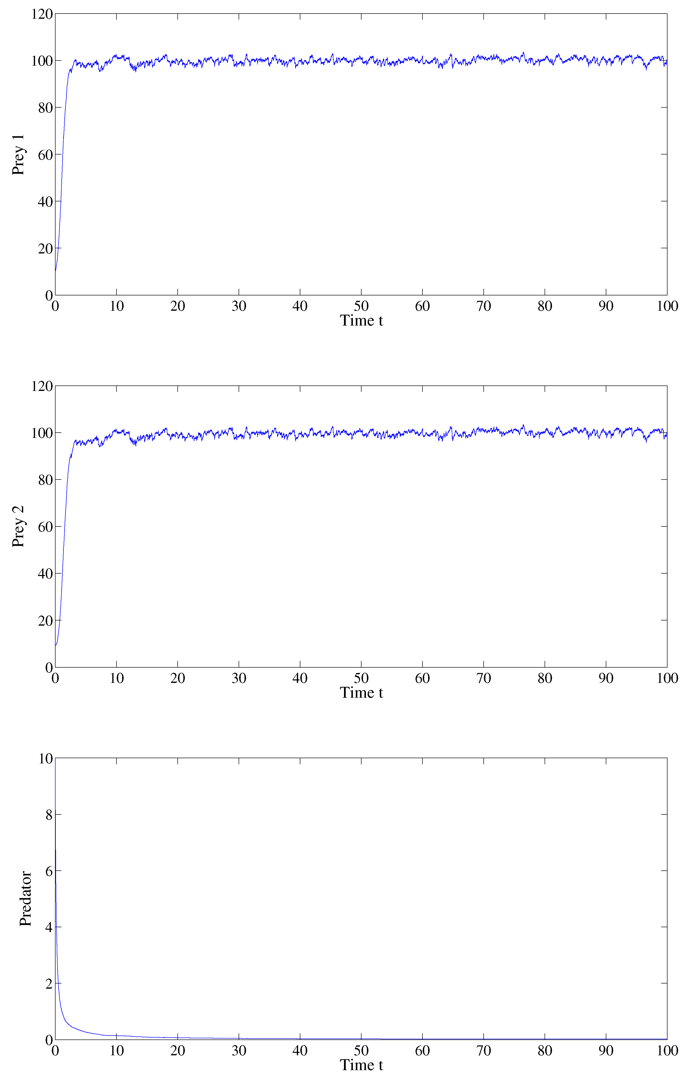
Figure 1 shows the evolution of the two prey, x and y, and the predator z, in the case that both prey and predator vanish. This means the extinction of the populations, which is in agreement with Section 3.
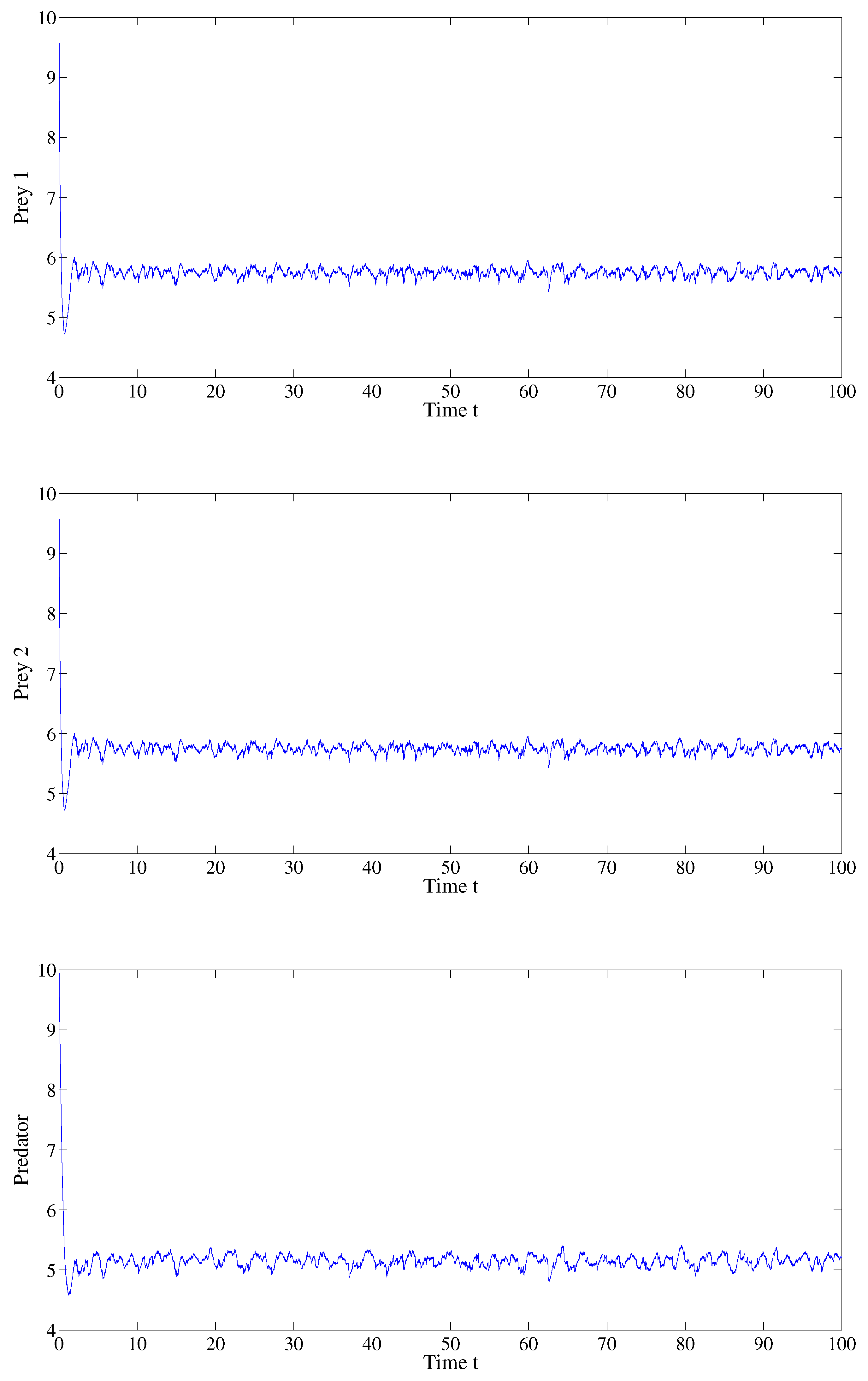
Figure 2 presents the dynamics of x, y and z in the case studied in Section 4, where the predator tends to zero and the prey remains strictly positive: the population of predators will be extinct while the population of prey persists.
Figure 3 illustrates the behavior of x, y and z in a situation where both the predator and the preys remain strictly positive, i.e., all populations persist. This agrees with our theoretical result of Section 5.
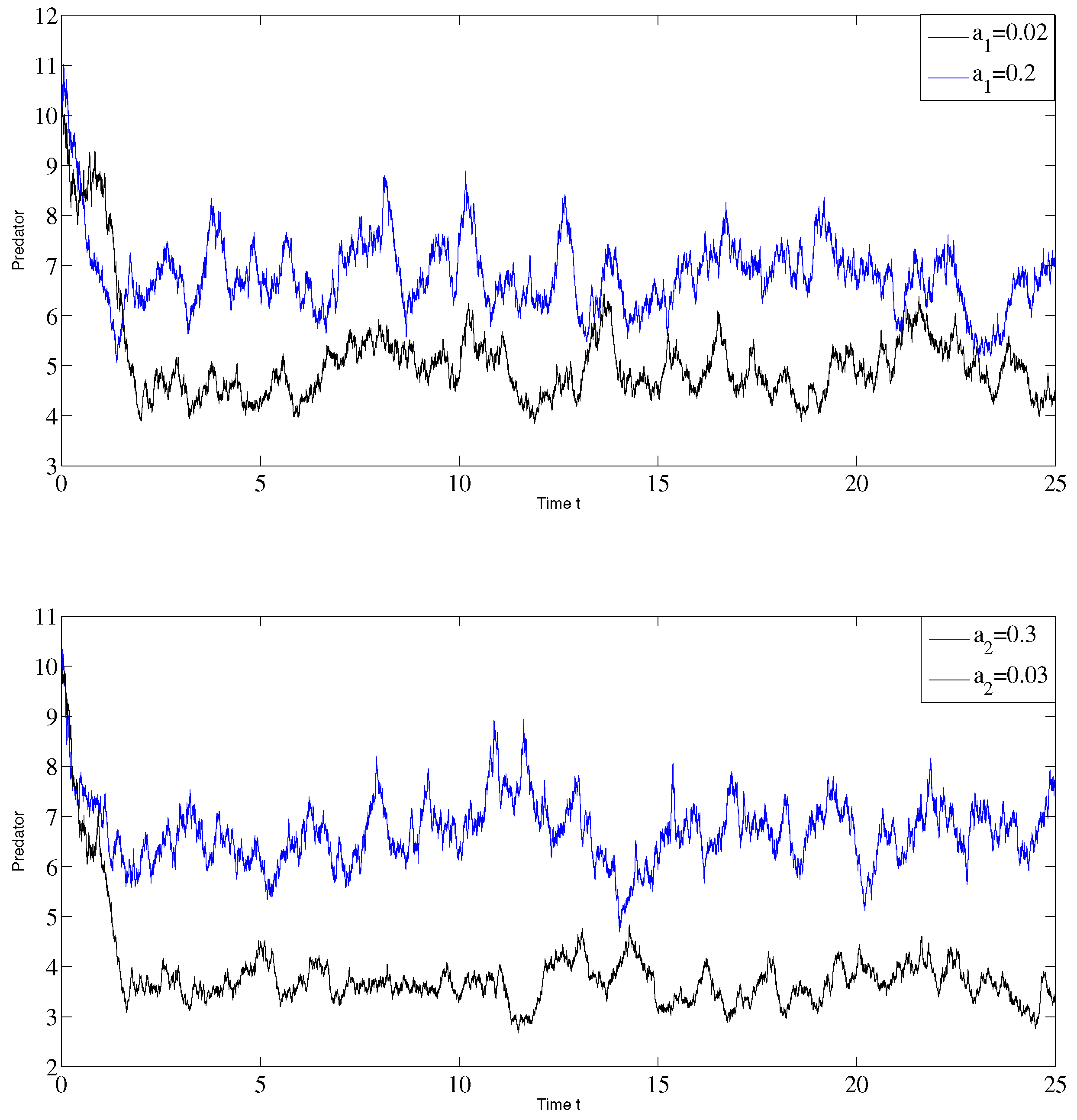
Figure 4 shows the impact of the transformation rates of predator to prey, a 1 and a 2 , based on the dynamics of the predator. We can remark that a 2 has more influence on the number of predators than the parameter a 1 .
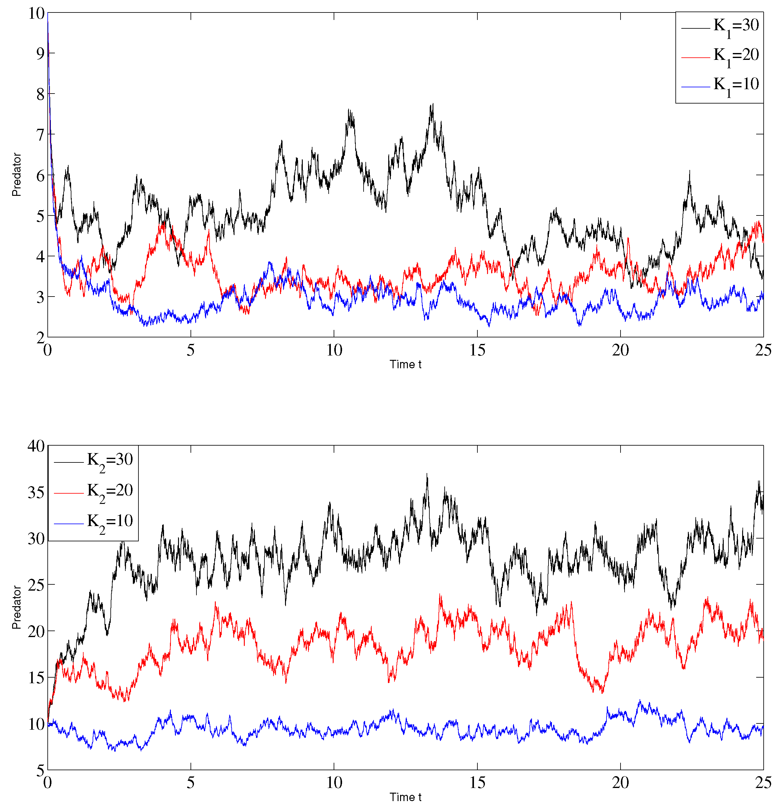
Figure 5 shows the impact of the carrying capacities K 1 and K 2 on the dynamics of the predator. We observe that K 2 has more influence on the number of predators than the parameter K 1 .
It is known that delays can affect the behavior of the studied population [31,32]. For this reason, now we study the effect of the delay on prey 1, prey 2, and the predator.
Figure 6 represents the dynamics of prey 1 for different values of τ 1 . We observe that when one increases the value of τ 1 from 0.5 to 2 days, that increases the amplitude of the prey 1 with a delay translation.
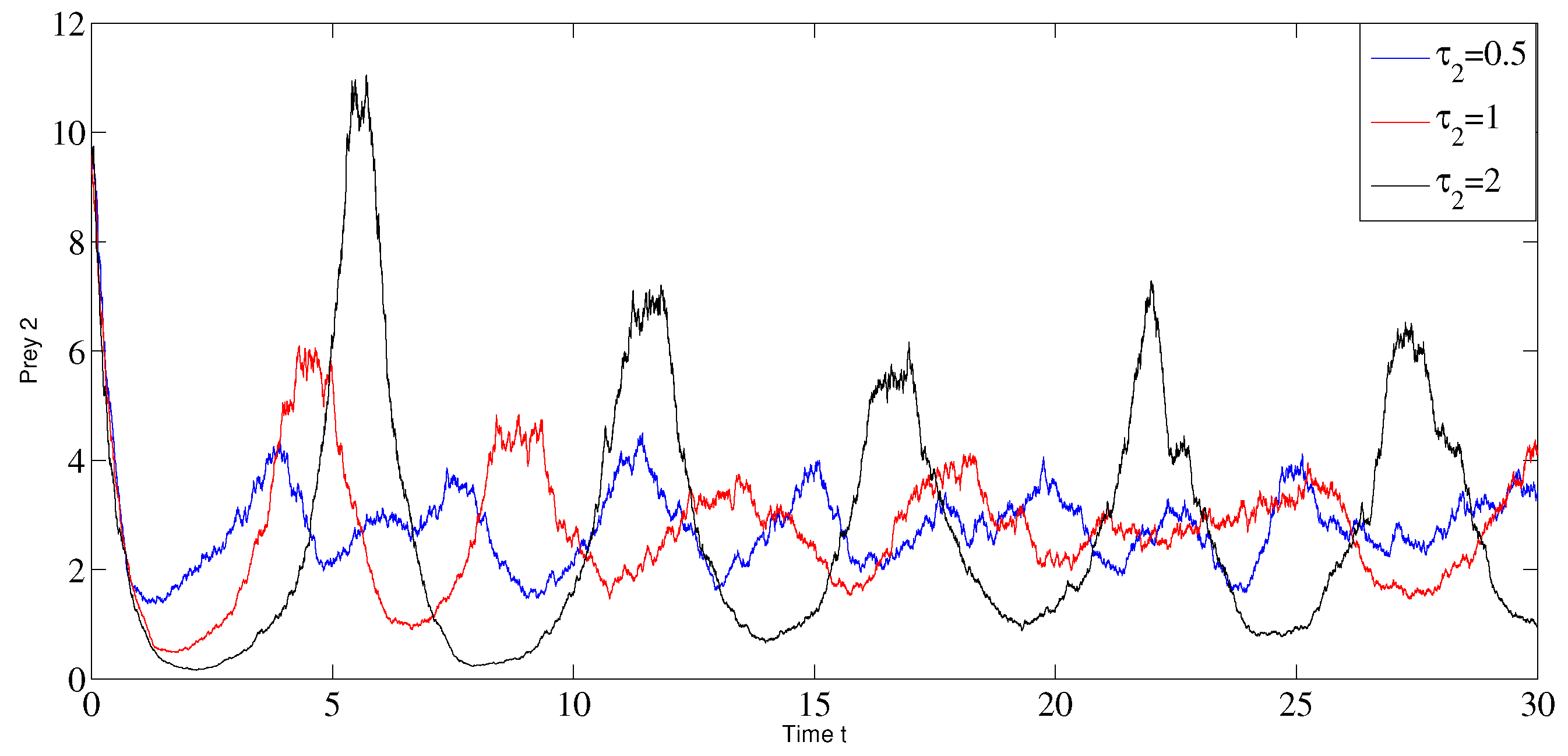
Figure 7 represents the dynamics of prey 2 for different values of τ 2 . We conclude that if we increase the value of τ 2 from 0.5 to 2 days, then the amplitude of the prey 2 increases with a delayed translation.
In Figure 8, we show the behavior of the predator population for different values of τ 3 . We note that an increase of the value of τ 3 from 0.5 to 2 days results in an increase of the amplitude of the predators with a delayed response.
Finally, in Figure 9 we illustrate the effect of the three delays. We observe that an increase on the values of τ 1 , τ 2 and τ 3 from 0.5 to 1 day implies an increase in the amplitude of all the populations with a translation.

7. Conclusions and Discussion

In this paper, we have proposed and analyzed a three-compartment model that depicts the interaction between two prey and one predator. The new stochastic predator–prey model incorporates Lévy noise and considers time delays of the two prey in the logistic functional production and in the transformation rate of predator to prey. Both white noise and Lévy jump perturbations are integrated into all model compartments. We have established the existence and uniqueness of a global positive solution and its boundedness, demonstrating the well-posedness of our stochastic predator–prey mathematical model. We have also provided sufficient conditions for the extinction of both prey and predator as well as for the persistence of the prey with the extinction of the predator. Additionally, we have presented a sufficient condition for the persistence in mean of both prey and the predator. Our theoretical findings are reinforced by different numerical results, demonstrating three possible scenarios: (i) the extinction of both prey and predator populations, (ii) the persistence of the prey and the extinction of the predator, and (iii) biological persistence, which is vital for maintaining the continuity of the reaction between prey and predator.
Several interesting research questions require further investigation in future studies. Specifically, our team intends to examine the spatial diffusion of a delayed prey–predator problem with Lévy jumps. Additionally, we plan to explore the bifurcation and chaotic behavior of the stochastic time-delayed prey–predator model. A comprehensive analysis is nontrivial and requires further inquiry, which we will undertake in another study. Furthermore, our analysis of the model under consideration can be expanded to include fractional-order derivative models, as described in [33,34], and we can explore alternative views of stochasticity, as demonstrated by the authors of [35]. We also note that the parameter values presented in Table 2 for numerical simulations of our theoretical results may not be applicable to real-world problems. Future research should strive to establish a connection with practical objectives and address the challenge of parameter estimation.

Author Contributions

Conceptualization, J.D. and D.F.M.T.; methodology, J.D. and D.F.M.T.; software, J.D.; validation, J.D. and D.F.M.T.; formal analysis, J.D. and D.F.M.T.; investigation, J.D. and D.F.M.T.; writing—original draft preparation, J.D. and D.F.M.T.; writing—review and editing, J.D. and D.F.M.T.; visualization, J.D.; project administration, D.F.M.T. All authors have read and agreed to the published version of the manuscript.

Funding

This research was funded by The Portuguese Foundation for Science and Technology (FCT) grant numbers UIDB/04106/2020 and UIDP/04106/2020.

Institutional Review Board Statement

Not applicable.

Informed Consent Statement

Not applicable.

Data Availability Statement

No new data were created or analyzed in this study. Data sharing is not applicable to this article.

Acknowledgments

The authors are very grateful to three anonymous referees for reading carefully the submitted manuscript and providing several valuable suggestions and comments.

Conflicts of Interest

The authors declare no conflict of interest. The funders had no role in the design of the study; in the collection, analyses, or interpretation of data; in the writing of the manuscript; or in the decision to publish the results.

References

  1. Tripathi, J.P.; Tyagi, S.; Abbas, Ṡ. Global analysis of a delayed density dependent predator-prey model with Crowley-Martin functional response. Commun. Nonlinear Sci. Numer. Simul. 2016, 30, 45–69. [Google Scholar] [CrossRef]
  2. Meng, X.-Y.; Huo, H.-F.; Xiang, H.; Yin, Q.-Y. Stability in a predator-prey model with Crowley-Martin function and stage structure for prey. Appl. Math. Comput. 2014, 232, 810–819. [Google Scholar] [CrossRef]
  3. Liu, Q.; Jiang, D.; Hayat, T.; Alsaedi, Ȧ. Dynamics of a stochastic predator-prey model with stage structure for predator and Holling type II functional response. J. Nonlinear Sci. 2018, 28, 1151–1187. [Google Scholar] [CrossRef]
  4. Lotka, A.J. Elements of Physical Biology; Dover: New York, NY, USA, 1956. [Google Scholar]
  5. Fay, T.H.; Greeff, J.C. Lion, wildebeest and zebra: A predator-prey model. Ecol. Model. 2006, 196, 237–244. [Google Scholar] [CrossRef]
  6. Spencer, P.D.; Collie, J.S. A simple predator-prey model of exploited marine fish populations incorporating alternative prey. Ices J. Mar. Sci. 1996, 53, 615–628. [Google Scholar] [CrossRef]
  7. Verhulst, P.-F. Notice sur la loi que la population suit dans son accroissement. Corresp. Math. Phys. 1838, 10, 113–121. [Google Scholar] [CrossRef]
  8. Edelstein-Keshet, L. Mathematical Models in Biology; Society for Industrial and Applied Mathematics (SIAM): Philadelphia, PA, USA, 2005. [Google Scholar] [CrossRef]
  9. Kingsland, S. The refractory model: The logistic curve and the history of population ecology. Q. Rev. Biol. 1982, 57, 29–52. [Google Scholar] [CrossRef]
  10. Kot, M. Elements of Mathematical Ecology; Cambridge University Press: Cambridge, UK, 2001. [Google Scholar] [CrossRef] [Green Version]
  11. MacLean, M.C.; Turner, Ȧ.W. The logistic curve applied to Canada’s population. Can. J. Econ. Polit. Sci. 1937, 3, 241–248. [Google Scholar] [CrossRef]
  12. Pearl, R.; Reed, Ŀ.J. The logistic curve and the census count of i930. Science 1930, 72, 399–401. [Google Scholar] [CrossRef]
  13. Abraha, T.; Basir, F.A.; Obsu, L.L.; Torres, D.F.M. Pest control using farming awareness: Impact of time delays and optimal use of biopesticides. Chaos Solitons Fractals 2021, 146, 11. [Google Scholar] [CrossRef]
  14. Arino, J.; Wang, L.; Wolkowicz, G.S.K. An alternative formulation for a delayed logistic equation. J. Theor. Biol. 2006, 241, 109–119. [Google Scholar] [CrossRef] [PubMed]
  15. Hutchinson, G.E. Circular causal systems in ecology. Ann. N. Y. Acad. Sci. 1948, 50, 221–246. [Google Scholar] [CrossRef] [PubMed]
  16. Kundu, S.; Maitra, S. Dynamical behaviour of a delayed three species predator-prey model with cooperation among the prey species. Nonlinear Dyn. 2018, 92, 627–643. [Google Scholar] [CrossRef]
  17. Rihan, F.A.; Alsakaji, H.J. Stochastic delay differential equations of three-species prey-predator system with cooperation among prey species. Discrete Contin. Dyn. Syst. Ser. S 2022, 15, 245–263. [Google Scholar] [CrossRef]
  18. Choo, S.; Kim, Y.-H. Global stability in stochastic difference equations for predator-prey models. J. Comput. Anal. Appl. 2017, 23, 462–486. [Google Scholar]
  19. Yang, L.; Zhong, S. Global stability of a stage-structured predator-prey model with stochastic perturbation. Discrete Dyn. Nat. Soc. 2014, 2014, 8. [Google Scholar] [CrossRef] [Green Version]
  20. Zhao, S.; Song, M. A stochastic predator-prey system with stage structure for predator. Abstr. Appl. Anal. 2014, 2014, 7. [Google Scholar] [CrossRef]
  21. Danane, J.; Allali, K.; Hammouch, Z.; Nisar, K.S. Mathematical analysis and simulation of a stochastic COVID-19 Lévy jump model with isolation strategy. Results Phys. 2021, 23, 12. [Google Scholar] [CrossRef]
  22. Akdim, K.; Ez-zetouni, A.; Danane, J.; Allali, K. Stochastic viral infection model with lytic and nonlytic immune responses driven by Lévy noise. Phys. A 2020, 549, 11. [Google Scholar] [CrossRef]
  23. Danane, J. Stochastic predator-prey Lévy jump model with Crowley-Martin functional response and stage structure. J. Appl. Math. Comput. 2021, 67, 41–67. [Google Scholar] [CrossRef]
  24. Zhang, X.; Li, W.; Liu, M.; Wang, K. Dynamics of a stochastic Holling II one-predator two-prey system with jumps. Phys. A 2015, 421, 571–582. [Google Scholar] [CrossRef]
  25. Liu, Q.; Chen, Q. Analysis of a stochastic delay predator-prey system with jumps in a polluted environment. Appl. Math. Comput. 2014, 242, 90–100. [Google Scholar] [CrossRef]
  26. Liu, M.; Bai, C.; Deng, M.; Du, B. Analysis of stochastic two-prey one-predator model with Lévy jumps. Phys. A 2016, 445, 176–188. [Google Scholar] [CrossRef]
  27. Zhao, Y.; Yuan, S. Stability in distribution of a stochastic hybrid competitive Lotka-Volterra model with Lévy jumps. Chaos Solitons Fractals 2016, 85, 98–109. [Google Scholar] [CrossRef]
  28. Wu, J. Stability of a three-species stochastic delay predator-prey system with Lévy noise. Phys. A 2018, 502, 492–505. [Google Scholar] [CrossRef]
  29. Øksendal, B.K.; Sulem, A. Applied Stochastic Control of Jump Diffusions, 3rd ed.; Universitext Series; Springer: Berlin/Heidelberg, Germany, 2009. [Google Scholar] [CrossRef]
  30. Zou, X.; Wang, K. Numerical simulations and modeling for stochastic biological systems with jumps. Commun. Nonlinear Sci. Numer. Simul. 2014, 19, 1557–1568. [Google Scholar] [CrossRef]
  31. Shao, Y.; Kong, W. A predator-prey model with Beddington-DeAngelis functional response and multiple delays in deterministic and stochastic environments. Mathematics 2022, 10, 3378. [Google Scholar] [CrossRef]
  32. Shao, Y. Dynamics of an impulsive stochastic predator-prey system with the Beddington-DeAngelis functional response. Axioms 2021, 10, 323. [Google Scholar] [CrossRef]
  33. Gholami, M.; Ghaziani, R.K.; Eskandari, Z. Three-dimensional fractional system with the stability condition and chaos control. Math. Model. Numer. Simul. Appl. 2022, 2, 41–47. [Google Scholar] [CrossRef]
  34. Yavuz, M.; Sene, N. Stability analysis and numerical computation of the fractional predator-prey model with the harvesting rate. Fractal Fract. 2020, 4, 35. [Google Scholar] [CrossRef]
  35. Naim, M.; Sabbar, Y.; Zeb, A. Stability characterization of a fractional-order viral system with the non-cytolytic immune assumption. Math. Model. Numer. Simul. Appl. 2022, 2, 164–176. [Google Scholar] [CrossRef]
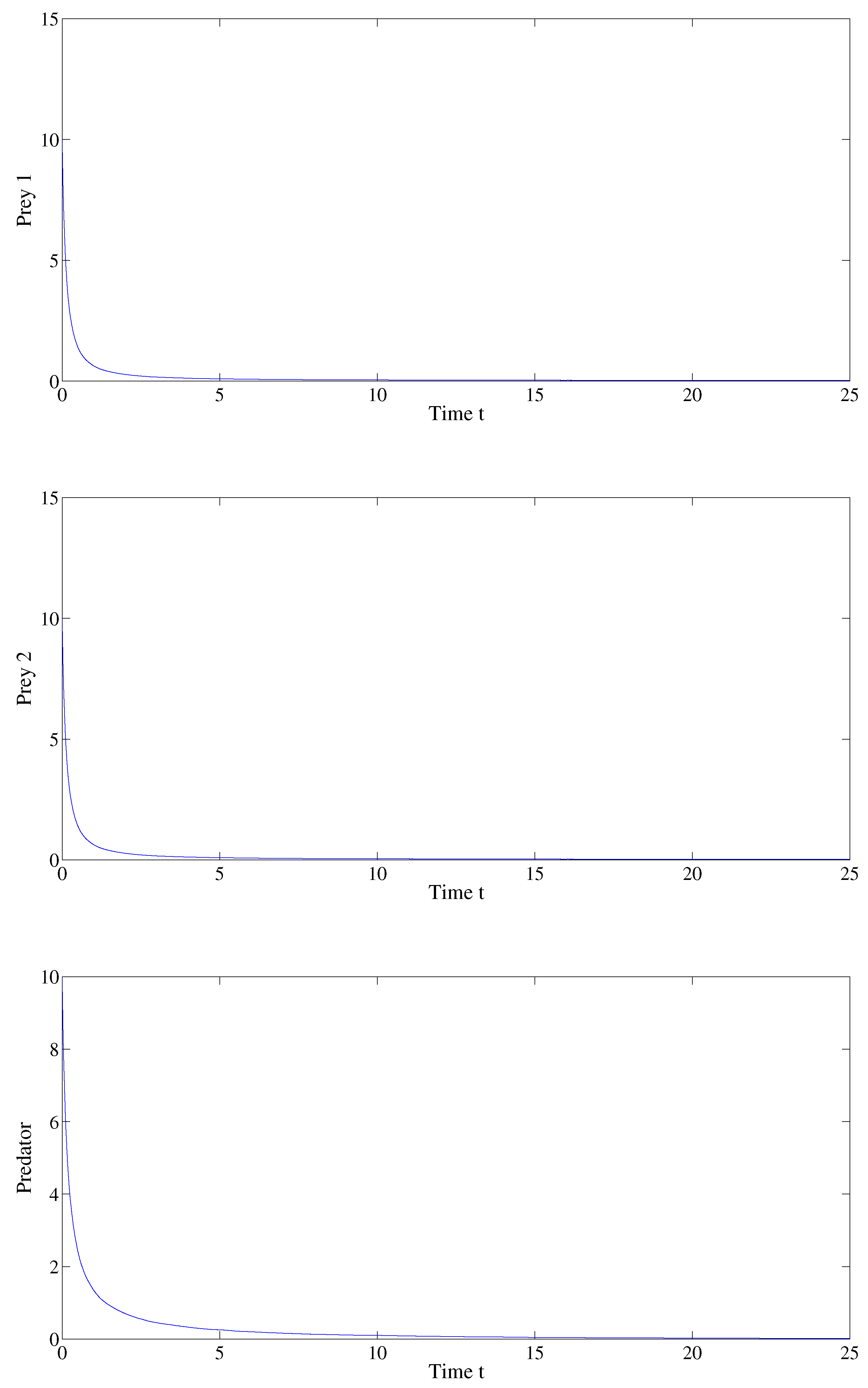
Figure 1. The behavior of the prey and predator populations in the extinction situation described by Theorem 3.
Mathematics 11 01595 g001
Figure 2. The behavior of the prey and predator populations in the extinction–persistence situation described by Theorem 4.
Mathematics 11 01595 g002
Figure 3. The behavior of the prey and predator populations in the case of persistence described by Theorem 5.
Mathematics 11 01595 g003
Figure 4. The behavior of the predator population for different values of a 1 and a 2 .
Mathematics 11 01595 g004
Figure 5. The behavior of the predator population for different values of K 1 and K 2 .
Mathematics 11 01595 g005
Figure 6. The behavior of the prey 1 population for different values of τ 1 .
Mathematics 11 01595 g006
Figure 7. The behavior of the prey 2 population for different values of τ 2 .
Mathematics 11 01595 g007
Figure 8. The behavior of the predator population for different values of τ 3 .
Mathematics 11 01595 g008
Figure 9. The behavior of the populations for different values of τ 1 , τ 2 and τ 3 .
Mathematics 11 01595 g009
Table 1. The description of the parameters for model (1).
ParametersDescription
r 1 The intrinsic growth rate for prey x
r 2 The intrinsic growth rate for prey y
K 1 The carrying capacity for x
K 2 The carrying capacity for y
α 1 The predation rate of prey x
α 2 The predation rate of prey y
β The rate of cooperation of preys x and y against predator z
δ The predator death rate
α 3 The rate of intra-species competition within the predators
a 1 The transformation rate of predator to preys x
a 2 The transformation rate of predator to preys y
Table 2. Values of the parameters used in the numerical simulations.
ParametersFigure 1Figure 2Figure 3
r 1 0.7 1.7 2
K 1 100100100
r 2 0.65 1.8 2.3
K 2 100100100
α 1 0.3 0.2 0.13
α 2 0.35 0.28 0.17
α 3 0.5 0.5 0.2
β 0.0001 0.0001 0.001
δ 0.1 0.4 0.02
τ 1 0.5 0.5 0.5
τ 2 111
τ 3 1.5 1.5 1.5
σ 1 10 4 10 5 10 5
σ 2 2 × 10 4 2 × 10 4 2 × 10 4
σ 3 2 × 10 4 2 × 10 3 2 × 10 3
q 1 ( u ) 0.04 0.04 0.04
q 2 ( u ) 0.006 0.006 0.006
q 3 ( u ) 0.008 0.008 0.008
Disclaimer/Publisher’s Note: The statements, opinions and data contained in all publications are solely those of the individual author(s) and contributor(s) and not of MDPI and/or the editor(s). MDPI and/or the editor(s) disclaim responsibility for any injury to people or property resulting from any ideas, methods, instructions or products referred to in the content.