Cooperative Control for Signalized Intersections in Intelligent Connected Vehicle Environments

Abstract

Cooperative control of vehicle trajectories and traffic signal phases is a promising approach to improving the efficiency and safety of transportation systems. This type of traffic flow control refers to the coordination and optimization of vehicle trajectories and traffic signal phases to reduce congestion, travel time, and fuel consumption. In this paper, we propose a cooperative control method that combines a model predictive control algorithm for adaptive traffic signal control and a trajectory construction algorithm. For traffic signal phase selection, the proposed modification of the adaptive traffic signal control algorithm combines the travel time obtained using either the vehicle trajectory or a deep neural network model and stop delays. The vehicle trajectory construction algorithm takes into account the predicted traffic signal phase to achieve cooperative control. To evaluate the method performance, numerical experiments have been conducted for three real-world scenarios in the SUMO simulation package. The experimental results show that the proposed cooperative control method can reduce the average fuel consumption by 1% to 4.2%, the average travel time by 1% to 5.3%, and the average stop delays to 27% for different simulation scenarios compared to the baseline methods.

1. Introduction

Transportation systems play an important role in the world economy. They provide freight transportation and facilitate supply chains, connect markets and resources, increase mobility and accessibility, etc. As a result, the development of transportation systems is necessary for the growth of the economy. According to [1], in 2021, transportation accounted for 8.4% of the gross domestic product in the U.S. Moreover, transportation-related industries employed almost 15 million people.

However, there are many challenges that can affect the efficient use of transportation networks. One of the main problems is congestion, which can lead to traffic delays, increased fuel consumption, and air pollution. With rising fuel prices, congestion had a significant negative economic impact on travel costs, freight transportation, and the supply chain, and increased the cost of goods and services around the world. According to [2], in the U.S., the typical driver lost 51 h due to traffic congestion in 2022, while in the UK it was around 80 h. This problem is even more acute in large cities. For example, in London, the most congested city in the world, drivers lost about 156 h on average due to congestion. In total, the cost of congestion was over $81 billion in the U.S. and more than £9 billion for UK drivers in 2022 [2]. Other problems in transportation systems include the negative impact of transportation on the environment due to air pollution and gas emissions, the need to improve passenger safety systems, such as the development of crash avoidance systems, and the need to modernize transportation infrastructure. Addressing these problems requires the development of innovative solutions such as intelligent transportation systems (ITS).

The intelligent transportation system is an advanced application that applies information and communication technologies for improving the efficiency, safety, and sustainability of transportation systems. ITSs provide tools for monitoring [3], traffic flow prediction [4,5], optimization [6] and control [7,8], public transport management [9], freight transportation [10], informing travelers [11], and so on. In [12], the authors studied the main stages of ITS development and reviewed the main works in the field of transportation engineering. It was concluded that ITSs can help transport agencies and regional departments improve their traffic management strategies in urban areas, as well as help commuters plan their trips and choose routes more efficiently.

Currently, the following directions of development of ITS can be distinguished. First, we note the development of the Internet of Things (IoT) ecosystem and smart cities. The integration of IoT devices into transportation systems is expected to play an important role in the future of ITS. Smart cities use advanced technologies such as sensors, cameras, and IoT devices to collect data on traffic flow, weather, and other factors that affect transport. This data can be used to optimize traffic flows, reduce emissions and improve the overall efficiency of transportation systems. Another significant milestone in the development of ITSs is the development of connected and autonomous vehicles (CAVs). Connected vehicles (CVs) can exchange information with other vehicles and with infrastructure, while autonomous vehicles (AVs) can use a wide range of sensors, cameras, and artificial intelligence techniques for driverless navigation. CAVs can reduce traffic accidents, improve road safety, reduce traffic congestion, and make transport more efficient overall.

Taking into account these factors, we can discuss the transition to cooperative ITS. Cooperative ITSs use communication and information technologies to improve transport systems by allowing vehicles, road infrastructure, and other road users to interact and exchange information in real-time. Examples of cooperative ITS applications include Advanced Traveler Information Systems (ATIS), Advanced Traffic Management Systems (ATMS), and Advanced Vehicle Safety Systems (AVSS).

In particular, this paper considers the problem of cooperative control of traffic signals and vehicle trajectories near signalized intersections. This type of traffic flow control refers to the coordination and optimization of vehicle trajectories and traffic signal phases to reduce congestion, travel time, and fuel consumption. Cooperative control can be achieved using advanced technologies such as Vehicle–to–Infrastructure (V2I) and Vehicle–to–Vehicle (V2V) communications in Vehicular Ad-hoc Networks (VANETs). The exchange of information between VANETs members must be secure and confidential [13]. Vehicles equipped with V2I or V2V communication systems can communicate with infrastructure objects and other connected vehicles to provide more accurate, safe, and efficient vehicle control. For example, if a vehicle ahead suddenly brakes, it can send a warning signal to the vehicle behind, enabling it to brake in time and avoid a collision. Another important task solved with the help of VANETs is the prediction of the motion state of nearby nonconnected vehicles [14]. The obtained predictions can be used for the safe movement of autonomous vehicles in mixed traffic flow environments and optimal route planning. V2I communication allows vehicles to communicate with infrastructure such as traffic signals and road sensors. For example, when a vehicle approaches an intersection, it can report its speed, position, and intended route. The traffic signal can then use this information to optimize green light phase times, reduce overall stop delays at the intersection, and improve traffic flow [15]. Similarly, vehicles can adjust their speed to reach the intersection during the green light phase and reduce stop delays. Cooperative control of vehicle trajectories and traffic signal phases is a promising approach for improving the efficiency and safety of transportation systems. This problem is now an active area of research and development in ITS.

The objective of this research is to develop and study a method for the coordinated control of traffic signals and vehicle trajectories in the intelligent connected vehicle environment. The proposed method consists of the following steps:

• Construction of vehicle trajectories with the condition that the intersection will be reached when the green traffic light is on;
• Estimation of the vehicle arrival time at the intersection, taking into account the vehicle trajectory or using a neural network prediction model;
• Assessment of the observed state of the transport network, including the stop delay for vehicles at the intersection and the arrival time at the intersection for each vehicle;
• Selection of the traffic signal phase based on the observed state using the selected adaptive traffic signal control algorithm; and
• Reconstruction of the vehicle trajectory, for which the predictive traffic signal phase has changed.

In step 4, it is proposed to use an adaptive traffic signal control algorithm that maximizes the predicted traffic flow through the intersection [16,17].

The contributions of this paper can be summarized as follows:

• A method of coordinated control of vehicle trajectories and traffic signals; and
• An algorithm for adaptive traffic signal control that maximizes the number of vehicles passing through the intersection, taking into account the trajectory of their movement and/or the arrival time at the intersection predicted by the neural network model.

The cooperative control method based on the model predictive control approach [17], which takes into account the trajectories of lead vehicles on intersection lanes, is new in the area of research on ITS based on our knowledge. Experimental results in the SUMO traffic simulation package [18], performed for three simulation scenarios, show the advantages of the proposed approach compared to the baseline methods.

The rest of the paper is organized as follows. Section 2 provides an overview of related works on the considered cooperative traffic signal control problem. Section 3 describes a cooperative control method, including a problem formulation, an adaptive traffic signal control algorithm, and a trajectory construction algorithm. In Section 4, we describe simulation scenarios and experimental results obtained using the SUMO microscopic traffic simulator that compares the effectiveness of the proposed method with the noncooperative and partially cooperative approaches. Finally, we discuss the obtained results, draw conclusions, and describe possible directions for further research in Section 5.

2. Related Works

The goal of a smart city transportation system is to provide residents with a range of transportation options that are safe, comfortable, and environmentally friendly. Smart city transportation systems use advanced technologies such as traffic sensors and intelligent traffic management systems to optimize traffic flow and reduce congestion. Intelligent connected vehicles (ICVs) are one of the most important elements of the traffic management system. ICVs are vehicles equipped with advanced communication and sensing technologies that enable them to communicate with other vehicles, pedestrians, and infrastructure. The authors of [19] presented a contract-based and priority transport management system. In the proposed transport management system, ICVs exchange information about their current motion states and the state of nearby nonconnected vehicles with each other and the traffic-managing center. This information is used to optimize the traffic flow of the transport network by the transport management system. In [20], the authors presented a method to solve the traffic optimization problem and applied it to optimize the energy consumption of vehicles in the transport network. In our work, we assume that all vehicles in the transport system are CAVs, and traffic flow optimization is achieved through the cooperation of an adaptive traffic signal control algorithm and a vehicle trajectory construction algorithm.

To provide an overview of the recent research papers on the cooperative traffic signal control problem, we sequentially consider three topics: adaptive traffic signal control, vehicle trajectory construction, and cooperative traffic signal control.

2.1. Traffic Signal Control

Traffic signal control (TSC) refers to the management of the timing and sequence of the traffic signal phases at intersections to optimize traffic flow and minimize congestion.

Early rule-based TSC methods used a set of predefined rules to control traffic signals, such as fixed-time control [21,22], actuated control [23,24,25], and adaptive control [7,26,27]. Rule-based methods are simple and easy to implement, but they can be inflexible and ineffective in environments where traffic changes rapidly.

The second class of traditional TSCs is optimization-based methods [28,29]. These methods consider the TSC problem as a multiobjective optimization problem and use mathematical optimization algorithms to find the optimal signal timing given various constraints and objectives such as minimizing delays and emissions and maximizing road capacity. Optimization-based methods are more flexible and can handle changing traffic conditions, but they are computationally complex and may require accurate environment models.

The third group of methods uses model predictive control (MPC) frameworks to predict various traffic flow characteristics that will be used to optimize traffic signal phases [17,30,31,32,33]. In [32], the authors used traffic volume prediction to calculate the optimal traffic signal phase split. In [30], using a simple macroscopic traffic model as input of the MPC framework was proposed. A point–queue model was considered in [31] to minimize the queue length for the TSC problem. In [17], the authors predicted the arrival time of each vehicle at an intersection with a deep neural network model and used this information to maximize the traffic flow through the intersection.

A more detailed survey of the traditional methods of adaptive and nonadaptive traffic signal control can be found in reviews [23,34,35].

Due to the active development of artificial intelligence and machine learning methods in the last decade, reinforcement learning methods have been extensively studied to solve the TSC problem [7,8,36,37]. Reinforcement learning (RL) is a type of machine learning in which an agent learns to make decisions by interacting with an environment. The agent interacts with the environment by performing an action based on an agent’s policy and an observed environment state and receives a reward based on the action taken. The goal of the agent is to learn the policy that maximizes the cumulative reward.

A representation of deep reinforcement learning (DRL) models (including state, action, and reward definitions) applied to TSC has been summarized in [36]. In [8], the authors provided a survey of recent deep RL-based traffic control applications with a focus on traffic signal control applications. The paper summarizes existing works on this problem and classifies them by application type, control models, RL settings, and studied algorithms. The authors also discussed the challenges and open research directions and concluded that existing approaches still need to be examined in real-world environments. The paper [37] provides a literature review on the TSC problem and discusses the challenges of synchronized TSC between adjacent signalized intersections.

RL algorithms can be classified into several types depending on learning approaches: value-based, policy-based, and actor–critic methods.

Q–learning is a value-based algorithm that estimates the expected reward of performing a certain action in a certain state using Q-values [38]. This approach can be used in scenarios with a small number of states and actions. To handle the high-dimensional state space problem, in a Deep Q–Networks (DQN) approach, it was proposed Q–Learning be combined with deep neural networks to represent Q–values [39,40,41,42,43]. A combination of a DQN model with a coordination algorithm was investigated in [39]. In [40], the authors proposed a cooperative DRL framework that controls traffic signals in a region using multiple regional agents and a centralized global agent. A DRL algorithm that extracts useful features from traffic data to learn the optimal policy was described in [41]. In [42], the authors proposed a novel DQN model, a state representation, and a reward definition to optimize traffic signal control in a partially observable environment with connected vehicles. In a Double DQN approach, it was proposed using two separate neural networks to estimate Q-values and select the best action [44,45]. This approach addresses the overfitting problem and shows more stable behavior in complex scenarios.

The second class of RL algorithms includes policy gradient methods. Policy-based algorithms directly optimize the policy, which is a probability distribution of action–state pairs, by updating the policy parameters based on the gradient of the expected reward [46,47,48]. In [46], the authors evaluated a deep deterministic policy gradient algorithm. The paper [47] investigated a proximal policy optimization (PPO) algorithm with variable time intervals for traffic signal phases. In [48], the authors proposed a modified PPO algorithm aimed at better adaptation to traffic conditions.

Actor–Critic methods are a combination of value-based and policy-based algorithms. In these methods, the actor represents a policy function that is used to select actions, and the critic represents a value function, which evaluates the actions performed by the actor [49,50,51,52]. In [50], the authors presented a multiagent RL method for adaptive TSC based on an advantage actor–critic algorithm (A2C). In [51], the authors integrated the deep neural network model that evaluates an environment state from a series of image representations of the intersection into an actor–critic model. Evaluation of different state representations for TSC using an asynchronous advantage actor–critic (A3C) algorithm was performed in [52].

Despite the active development of RL methods for the TSC problem, these methods have several disadvantages. First, training RL algorithms to solve the TSC problem can be time-consuming and computationally intensive, especially for large and complex real-world scenarios. Second, RL algorithms often require accurate environment models to learn the optimal policy. However, in real-world scenarios, obtaining accurate and complete information about the environment state can be challenging. Finally, it can be difficult to generalize RL algorithms to new situations, especially when the state and action spaces are large or when the environment changes significantly.

As a result, in this paper, the MPC-based method [17] is used as the base adaptive TSC algorithm.

2.2. Trajectory Construction

The optimal vehicle trajectory construction is necessary to prevent acceleration and deceleration of vehicles near traffic signals at intersections. This “stop–and–go” traffic pattern has several disadvantages, including increased fuel consumption and emissions, increased travel delays, decreased intersection capacity, and increased risk of accidents. In a connected vehicle environment, it is possible to slow down in advance to avoid stops and queues at intersections, reduce travel delays and fuel consumption, and improve the efficiency of the transportation system.

In [53] the authors evaluated an approach for trajectory identification from closed-circuit television (CCTV) video. The paper [54] describes a model for predicting the passage time of a queue of vehicles at a signalized intersection. Using this model, the authors proposed an approach for choosing an optimal speed mode to reduce the number of stops of connected vehicles.

In [55], the authors presented an optimization model designed to distribute the arrival time of vehicles at the intersection and minimize network delays. In [33], a time–velocity planning problem with constraint was formulated and solved to obtain a smooth trajectory, taking into account the velocity plan and longitudinal dynamics control. The paper [56] formulated a two-stage model that optimizes a trajectory of the longitudinal and lateral behavior of CAVs along a signalized arterial under a mixed traffic environment. In [57], the authors described heuristic algorithms for trajectory design that decompose a hard trajectory construction problem into a simple constructive heuristic. It was shown that the proposed algorithms allow us to find a feasible solution to the original problem. The computation complexity and optimality of the proposed algorithm were evaluated in [58].

In this paper, we use a modified version of the algorithm proposed in [57] to construct vehicle trajectories, taking into account speed, acceleration, distance to an intersection, and a traffic signal phase.

2.3. Cooperative Control

In this subsection, we provide an overview of the research papers on coordinated signal optimization and CAVs trajectory control.

A review of cooperative control methods in a connected vehicle environment was presented in [59]. The authors provided an overview of existing approaches, typical traffic control scenarios, and active and indirect control strategies and concluded that improved coordinated control in a hybrid traffic flow could significantly improve traffic efficiency.

In [17], the authors proposed a cooperative traffic signal control method in which a trajectory optimization algorithm takes into account the predicted traffic signal phase. However, an adaptive TSC algorithm did not take into account vehicle trajectories. The two-stage model for signal optimization and trajectory control was presented in [60]. In the first stage, an algorithm based on a recurrent long short-term memory (LSTM) neural network is used to predict driver behavior. In the second stage, this information is used as an input for the DRL model of signal optimization. In [61], the authors proposed a coupled control method in a mixed traffic environment to optimize the timing of traffic signal phases and CAV trajectories to reduce energy consumption. However, an experimental study of the method was conducted on a synthetic scenario with one intersection. In [62], a methodology for coordinated traffic signal control and trajectory optimization was proposed, formulated as a mixed-integer nonlinear program. The proposed approach is applicable only to intersections with exclusive left-turn movements.

This study presents a method for cooperative traffic signal control and trajectory optimization under a connected vehicle environment. In the next section, we present the problem statement and description of the developed method.

3. Cooperative Control Method

To describe the proposed method for cooperative traffic signals optimization and CAVs trajectory control, we sequentially describe its main parts: the adaptive traffic signal control algorithm, the trajectory construction algorithm, and the cooperative control method that combines these algorithms.

3.1. Problem Formulation

The main objective of cooperative control of vehicle trajectories and traffic signals is to optimize the traffic flow and increase the efficiency of the transportation system. To achieve these objectives, the following metrics are usually considered: traffic delay and fuel consumption. The key objective is to minimize travel time for vehicles, including by reducing stop delays at intersections, as this reduces congestion and enhances driver mobility. The second important criterion is fuel consumption reduction, as this can help reduce emissions and increase the energy efficiency of the transportation system.

The cooperative control problem can be formulated as follows:

$$\lambda ·Travel{T}_{\sum }\left(A_{TS},A_{Tr}\right)+\eta ·Delay{T}_{\sum }\left(A_{TS},A_{Tr}\right)+\delta ·Fuel{C}_{\sum }\left(A_{TS},A_{Tr}\right)\to \underset{A_{TS},A_{Tr}}{\min },$$

(1)

where $Travel{T}_{\sum }\left(A{T}_S,A_{Tr}\right)$ is the total travel time of all vehicles at the intersection, $Delay{T}_{\sum }\left(A_{TS},A_{Tr}\right)$ is the total stop delays of all vehicles at the intersection; $Fuel{C}_{\sum }\left(A_{TS},A_{Tr}\right)$ is the total fuel consumption by all vehicles; and $\lambda ,\eta ,\delta$ are weight coefficients that jointly characterize the relative importance of a particular factor. To solve this problem, the adaptive traffic signal control algorithm and the trajectory construction algorithm are used.

3.2. Adaptive Traffic Signal Control

3.2.1. MPC-Based Algorithm

To solve the adaptive traffic signal control problem, this paper proposes using the algorithm based on a model predictive control approach [17]. The algorithm consists of two stages. In the first stage, the number of vehicles passing through the intersection for each traffic signal phase is estimated. In the second stage, a phase is selected that maximizes the traffic flow and minimizes the stop delays.

Let us give a formal description of the algorithm in the pseudocode form. Introduce the following notation. We define $P$ as the set of traffic signal phases, ${\tau }_{\min }$ as a minimum phase switching interval, $t_{cur}$ as the duration of the current (active) phase $p_{cur}\in P$ of the traffic signal, and $p_{out}\in P$ as the selected (switching) phase. Using these notations, the adaptive TSC algorithm based on maximizing the predicted weighted traffic flow (denoted below as MaxPWFlow) can be defined as follows (Algorithm 1).

Algorithm 1: MaxPWFlow algorithm

1: Input data: ${\tau }_{\min }, t_{cur}, p_{cur}, P$ 2: Output data: $p_{out}$ 3: if ${\mathit{t}}_{\mathit{c}\mathit{u}\mathit{r}}<{\mathbf{\tau }}_{\mathit{m}\mathit{i}\mathit{n}}$ then 4:   $p_{out}=p_{cur}$ 5:   $t_{cur}=t_{cur}+1$ 6: else 7:   $p_{out}=\arg \max \left(\left\{PWFlow\left(p\right) \mathrm{for} p \mathrm{in} P\right\}\right)$ 8:   $t_{cur}=0$ 9: end if

The main step of the algorithm is the prediction of traffic flow characteristics in function $PredFlow$, which represents traffic demand and is used to optimize the traffic signal phases. In this paper, it is proposed using two characteristics: the number of vehicles crossing the intersection during the time interval of the next phase and the stop delay of vehicles at the intersection. As a result, function $PredFlow\left(p\right)$ for given phase $p\in P$ is defined as follows:

$$PWFlow\left(p\right)={\displaystyle \sum _{l\in L_p^{income}}{\displaystyle \sum _{c\in C_l}\eta }}\left(c,l\right)I\left(T_o^{pnext}\le t\left(c\right)<T_o^{pnext}+{\tau }_{min}\right),$$

(2)

where $L_p^{income}$ is the set of lanes with allowed movements when phase $p\in P$ is on, $C_l$ is the set of vehicles on lane $l$, $T_o^{pnext}$ is the phase switching time, $t\left(c\right)$ is the time that vehicle $c\in C_l$ will cross the intersection, $\eta \left(c,l\right)$ is the coefficient that takes into account the stop delay of vehicle $c$ on lane $l$, and $I\left(val\right)$ is the indicator function:

$$I\left(val\right)=\{\begin{array}{c}1,val=True,\\ 0, \mathrm{otherwise}.\end{array}$$

(3)

Coefficient $\eta \left(c,l\right)$ is defined as follows:

$$\eta \left(c,l\right)=1+\alpha ·delay\left(c,l\right),$$

(4)

where $delay\left(c,l\right)$ is the stop delay of vehicle $c$ on lane $l$, and $\alpha =0.01$ is an experimentally chosen coefficient.

To estimate crossing time $t\left(c\right)$, we consider two options:

• For vehicles with the known (constructed) trajectory, the crossing time is calculated precisely according to the trajectory since the trajectory determines the vehicle speed at each time moment; and
• For other vehicles, the crossing time is estimated using a prediction model based on the deep neural network (DNN) model.

In this paper, we construct trajectories only for lead vehicles on signalized lanes closest to intersections. Other vehicles are controlled using a car-following model. This approach can significantly reduce computational resources. The original Shooting Heuristic algorithm constructs trajectories sequentially for all vehicles on the lane. According to the proposed cooperative control method (Section 3.4), the trajectory of the lead vehicle needs to be reconstructed in some cases. Therefore, it is necessary to sequentially reconstruct trajectories of all vehicles on the lane when using the original Shooting Heuristic algorithm. In addition, different types of vehicles allow us to apply the proposed method in a mixed traffic flow environment with CAV and connected human-driven vehicles. In this case, the trajectory is constructed only for the lead CAVs on signalized lanes.

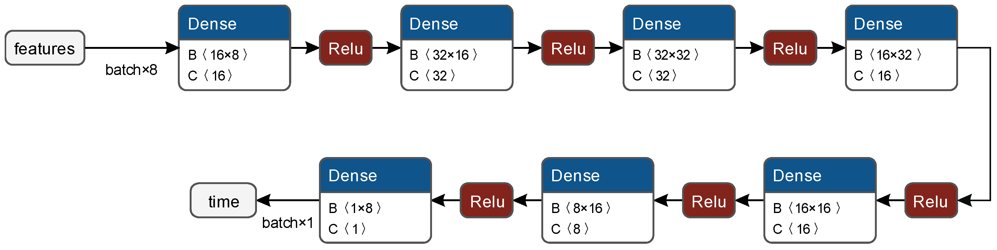
3.2.2. Crossing Time Prediction Algorithm

To predict the crossing time $t\left(c\right)$ of vehicle $c\in C_l$, we propose using a DNN-based model. As an input to the DNN model, a set of features describing the vehicle movement and the traffic state in the intersection area is used. The feature set includes:

• Distance from the current vehicle position to the intersection;
• Vehicle speed;
• Vehicle acceleration;
• Maximum allowed speed;
• Number of preceding vehicles;
• Type of the expected movement direction at the intersection; and
• Speed and position of the nearest vehicle on the outgoing lane.

The DNN model predicts the crossing time based on the defined input feature set.

The DNN model consists of seven dense layers. The architecture of the DNN model is shown in Figure 1.

All figures and tables should be cited in the main text as Figure 1,

Table 1. Simulation scenario parameters.

Scenario	Traffic Signals	Intersections	Segments	Trips
“Cologne-3”	3	29	48	2830
“Cologne-8”	8	78	149	1740
“Cologne-316”	316	2928	5808	13,530

, etc.

For the vehicle that is controlled directly, the crossing time is calculated based on its trajectory. In the next subsection, we describe the trajectory construction algorithm.

3.3. Trajectory Construction

To formulate the trajectory optimization problem, we introduce some notation. Let the considered vehicle $c\in C_l$ enter lane $l$ adjacent to the intersection in position $l_0$ at time $t_0$ with speed $v_0$. Denote the lane length as $L$, the maximum vehicle traveling speed on lane $l$ as $v_{\max }$, the maximum vehicle acceleration as $\overline{a}$, and the maximum vehicle deceleration as $\underset{\_}{a}$.

The vehicle trajectory $tr$ must be feasible and safe and satisfy the following constraints:

$$\begin{array}{l}tr\left(t_0\right)=l_0,\\ 0\le t{r}^{\prime }\left(t\right)\le v_{\max }, \underset{\_}{a}\le t{r}^{″}\left(t\right)\le \overline{a}, \forall t\in (-\infty ,+\infty ), \\ G\left(T\left(tr,L\right)\right)=T\left(tr,L\right),\end{array}$$

(5)

where $t{r}^{\prime }(t)$ is the first-order derivative (speed), $t{r}^{″}(t)$ is the second-order right derivative (acceleration), $T\left(tr,L\right)$ is the time that the vehicle will arrive at the intersection (i.e., reaches position $L$), and $G(t)$ is the function that returns the time when the green light for lane $l$ is on, greater than or equal to $t$. Function $G(t)$ can be defined as follows:

$$G(t)=\min \{t^{\prime }:t^{\prime }\ge t\wedge t^{\prime }\in \left[T_0+n{T}_c,T_0+n{T}_c+T_g\right),n\in {\mathbb{Z}}^{+}\},$$

(6)

where $T_o$ is the traffic signal cycle start time, $T_g,T_y,$ and $T_r$ are the durations of the green light, the yellow light, and the red light, respectively, $T_c=T_g+T_y+T_r$ is the duration of the traffic signal phase, and ${\mathbb{Z}}^{+}$ is the set of positive integers.

In this paper, a modified version of the Shooting Heuristic (SH) algorithm [57] is used to build the trajectory. We construct trajectories only for lead vehicles on signalized lanes closest to intersections. Other vehicles are controlled using a car-following model [18].

The first step of the algorithm is the Forward Shooting Process (FSP), which constructs a two-section trajectory. The first section describes a uniformly accelerated motion from the starting position described by the tuple $(t_0,v_0,l_0)$ until the cruising speed $v_{cruise}\in (0,v_{\max }]$ is reached. Traveling along the first section of the trajectory takes $(v_{cruise}-v_0)/{\overline{a}}^f$ seconds. The second section describes a uniform rectilinear motion with speed $v_{cruise}$ from time $t_0+(v_{cruise}-v_0)/{\overline{a}}^f$ until the vehicle enters the intersection. The vehicle enters the intersection at time ${\widehat{t}}_{}^{+}$ defined as follows:

$${\widehat{t}}_{}^{+}(v_{cruise},{\overline{a}}^f)=t_0+\{\begin{array}{l}\frac{-v_0-\sqrt{{(v_0)}^2+2{\overline{a}}^{f}L}}{{\overline{a}}^f}, if L\le \frac{v_{cruise}{}^2-{(v_0)}^2}{2{\overline{a}}^f},\\ \frac{L}{v_{cruise}}+\frac{{(v_{cruise}-v_0)}^2}{2{\overline{a}}^f{v}_{cruise}}, otherwise.\end{array}$$

(7)

The constructed trajectory $t{r}^f$ is required if the vehicle traveling along the trajectory enters the intersection with the green light on, i.e., the following condition is satisfied: $G\left(T\left(t{r}^f,L\right)\right)=T\left(t{r}^f,L\right)$. Otherwise, the second step of the SH algorithm is performed, which is called the Backward Shooting Process (BSP).

In the BSP step, trajectory $t{r}^f$ is revised. First, the second section of the trajectory is shifted along the time axis to the start of the next green phase $G({\widehat{t}}_{}^{+})$. This shifted section becomes the initial section of a modified trajectory $t{r}^b$. Sections of trajectory $t{r}^b$ are constructed from the initial section with acceleration ${\overline{a}}^b\in (0, \overline{a}]$ and deceleration ${\underset{\_}{a}}^b\in [\overline{a}, 0)$. Finally, the trajectories $t{r}^f$ and $t{r}^b$ merge into a feasible trajectory $tr$. The set of parameters $({\overline{a}}^f, {\overline{a}}^b,{\underset{\_}{a}}^b, v_{cruise})$ defines the smoothness of trajectory $tr$.

Figure 2 plots the time-space trajectories of the human-driven vehicles and CAV trajectories constructed using the SH algorithm.

To optimize the constructed trajectory $tr$, a weighted sum of several factors is used as the optimization objective function:

$$M(tr)=\lambda ·TravelT(tr)+\eta ·DelayT(tr)+\delta ·FuelC(tr),$$

(8)

where $TravelT(tr)$ is the travel time of the vehicle along trajectory $tr$, $DelayT(tr)$ is the stop delay, $FuelC(tr)$ is the fuel consumption along trajectory $tr$, and $\lambda ,\eta ,\delta$ are the weight coefficients.

To calculate the fuel consumption, we use the model based on data from [63]. According to the model, the fuel consumption at time moment $t$ depends on speed $v=t{r}^{\prime }\left(t\right)$ and acceleration $a=t{r}^{″}\left(t\right)$ of the vehicle [18]:

$$FuelC(tr(t))=\{\begin{array}{l}0,if a<0,\\ \frac{3014+v·(299.3·a-149+9.014·v)}{2671.2}, otherwise.\end{array}$$

(9)

The trajectory optimization problem can be formulated as follows:

$$\begin{array}{l}M(tr({\overline{a}}^f, {\overline{a}}^b,{\underset{\_}{a}}^b, v_{cruise}))\to \underset{{\overline{a}}^f, {\overline{a}}^b,{\underset{\_}{a}}^b, v_{cruise}}{\min },\\ 0<{\overline{a}}^f\le \overline{a}, 0<{\overline{a}}^b\le \overline{a},\\ \underset{\_}{a}\le {\underset{\_}{a}}^b<0, 0\le v_{cruise}\le v_{\max }.\end{array}$$

(10)

To solve the optimization problem, a subgradient algorithm was used [58]. In the first step, a set of control parameters $({\overline{a}}^f, {\overline{a}}^b,{\underset{\_}{a}}^b, v_{cruise})$ is selected from the trajectory constructed by the SH algorithm.

Then, the numerical subgradient is calculated by slightly changing the current control parameters. Next, the algorithm searches along the subgradient direction trying to minimize the objective function (N1). This numerical subgradient search process is repeated until certain terminal criteria (the maximum number of steps when searching along a gradient) are met.

The constructed optimal trajectory is used in the cooperative control method described in the next subsection.

3.4. Cooperative Control

The proposed cooperative control method combines the adaptive traffic signal control algorithm (described in Section 3.2) and the CAVs trajectory construction algorithm (described in Section 3.3).

To provide cooperative control, it is necessary to redefine function $G(t)$ used as the constraint in the vehicle trajectory algorithm (N0) in the BSP step. Since we consider adaptive traffic signal control, in which the time of the traffic signal cycle is not constant, the function definition (N2) cannot be used.

Let $p\in P$ be the active phase of the traffic signal, $p_{next}\in P$ be the predicted traffic signal phase obtained as a result of the adaptive TSC algorithm, and ${\tau }_{min}$ be the minimum phase switching interval. We define the start time of phase $p$ as $T_o^p$ and the start time of phase $p_{next}$ as $T_o^{pnext}=T_o^p+{\tau }_{\min }$. $c\left(p,l\right)\in \left\{green, yellow, red\right\}$ denotes the traffic light for phase $p$ and lane $l$.

Using this notation, we define function $G(t,l,p,p_{next})$ as follows:

$$G(t,l,p,p_{next})=\{\begin{array}{l}t, \mathrm{if} c\left(p,l\right)=green \wedge \left(c\left(p_{next},l\right)=green\vee t<T_o^{pnext}\right),\\ \max \left\{t,T_o^{pnext}\right\}, \mathrm{if} c\left(p,l\right)\ne green \wedge c\left(p_{next},l\right)=green,\\ \max \left\{t,T_o^{pnext}+{\tau }_{\min }\right\}, otherwise.\end{array}$$

(11)

The cooperative control method can be described as follows:

• Construct trajectories for all lead vehicles on each lane $l$ assuming $c\left(p_{next},l\right)=green$ for all lanes;
• Calculate the crossing time $t\left(c\right)$:
  • For the lead vehicles, $t\left(c\right)$ is calculated based on the constructed trajectory;
  • For other vehicles, $t\left(c\right)$ is calculated using the crossing time prediction algorithm described in Section 3.2.2;
• Select the next phase $p_{next}$ using the adaptive traffic signal control algorithm MaxPWFlow described in Section 3.2:
  • Calculate the traffic demand using (2);
  • Select the next phase that maximizes the traffic demand; and
• Given the predicted next phase $p_{next}$, reconstruct trajectories for all lead vehicles for which the assumption $c\left(p_{next},l\right)=green$ is not satisfied.

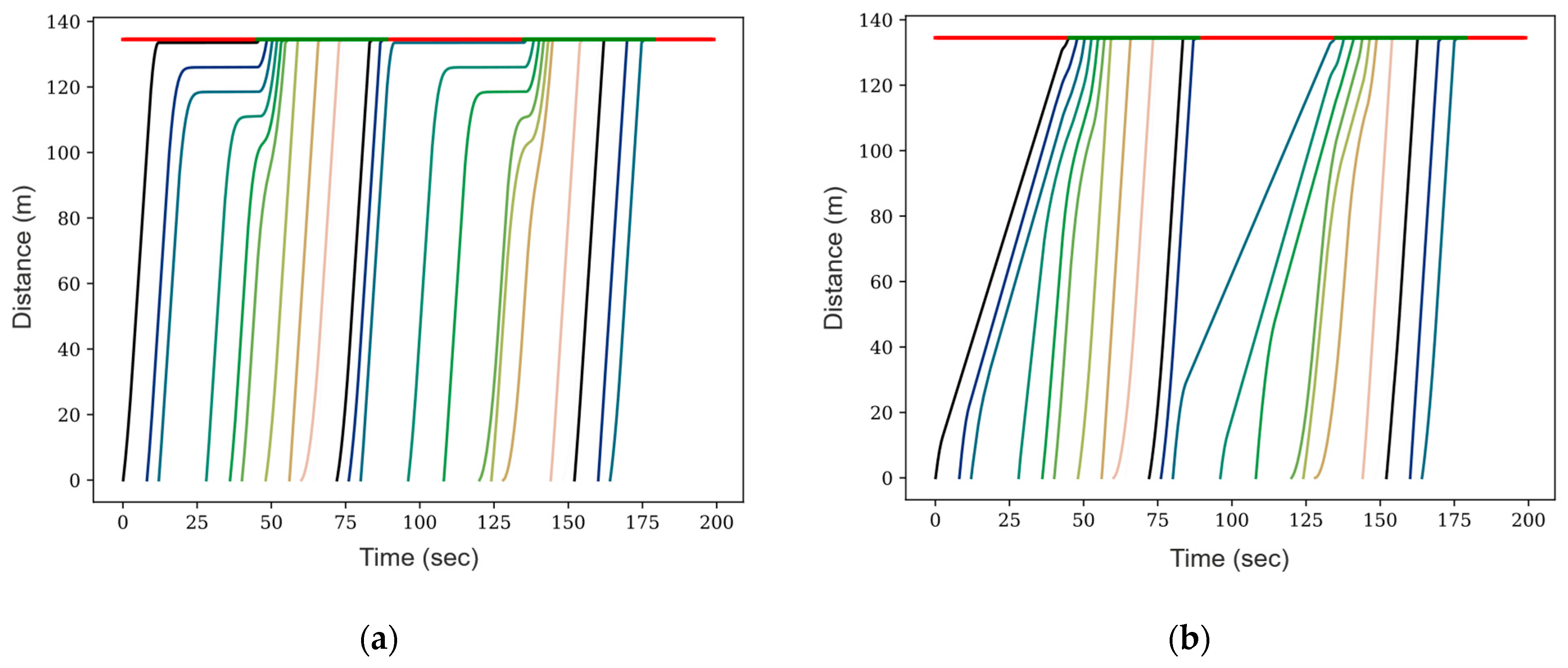
4. Experiments

The purpose of the experimental study was to evaluate the effectiveness of the proposed cooperative control method in real-world simulation scenarios. SUMO (Simulation of Urban MObility) [18] was used as the simulation platform. SUMO is an open-source traffic simulation package designed for the microscopic simulation of multimodal traffic scenarios in large-scale road networks. SUMO supports autonomous driving, vehicle communications, traffic management, traffic signal control, and other features.

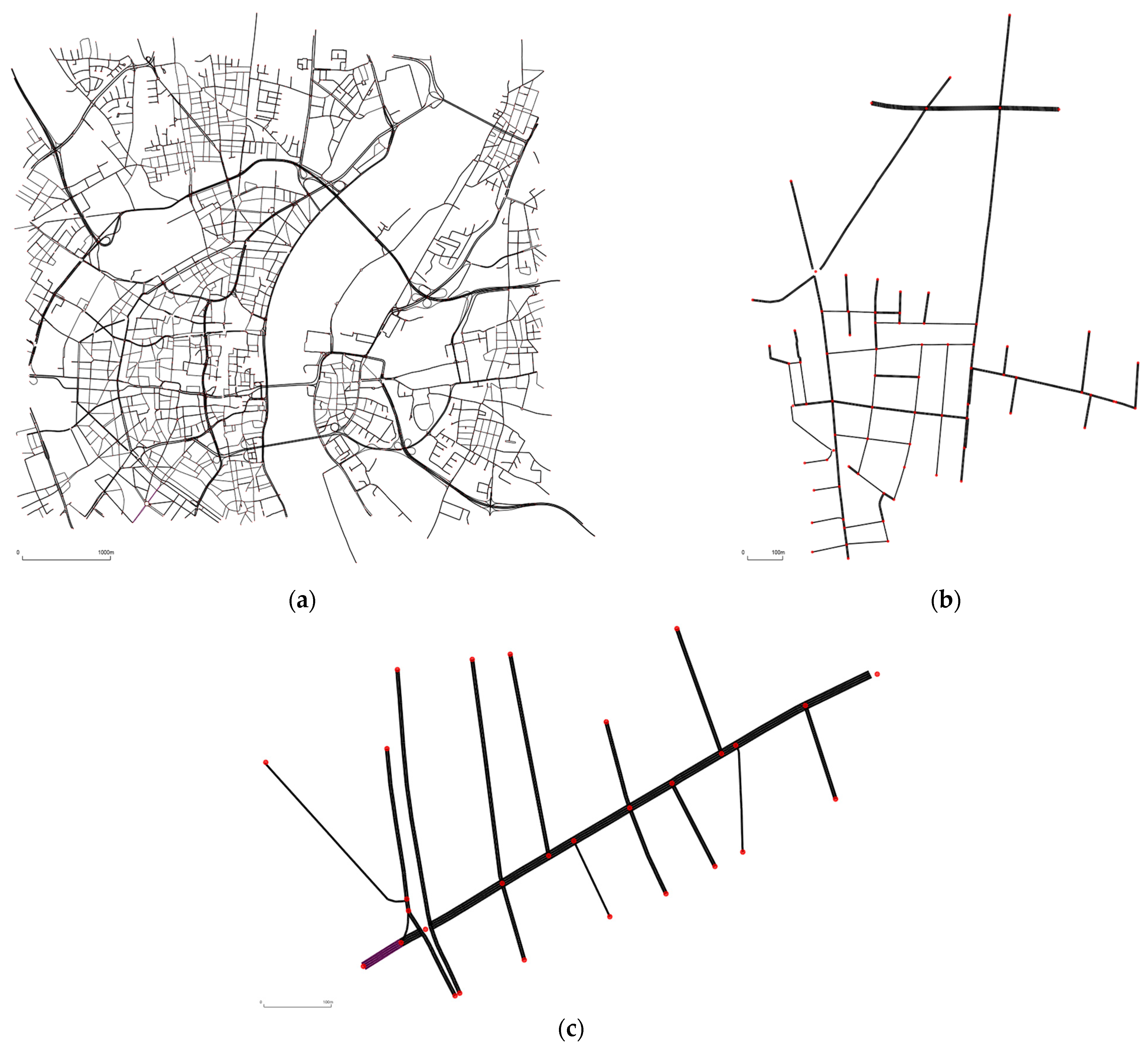
4.1. Case Study

We applied the proposed method to 3 simulation scenarios based on the well-established “TAPAS Cologne” SUMO scenario [64]:

• Simulation scenario in an arterial corridor “Cologne-3” [65];
• Simulation scenario in a small road network “Cologne-8” [65]; and
• Simulation scenario in a large road network “Cologne-316” [17].

The main scenario parameters are presented in Table 1.

Figure 3 shows the road networks of the described scenarios. Red dots represent intersections.

Each scenario was simulated in 10 episodes with 10 different random seeds. In each episode, the departure time and departure position when the vehicle entered the network were different.

In this study, we used 3 performance measurements to evaluate the effectiveness of the proposed method: the average travel time, the average stop delays, and the average fuel consumption.

4.2. Baseline Methods

In the experimental study, we compared the proposed cooperative control method with noncooperative adaptive traffic signal control strategies and semicooperative approaches in which the traffic signal phase is taken into account to construct the vehicle trajectory, but the trajectory is not used in adaptive traffic signal control. A direct comparison of the proposed method with other cooperative control approaches is difficult for several reasons: existing algorithms do not provide source code or datasets for comparison, use different traffic simulation software tools, ignore lane changes, etc.

Namely, we compared the following methods:

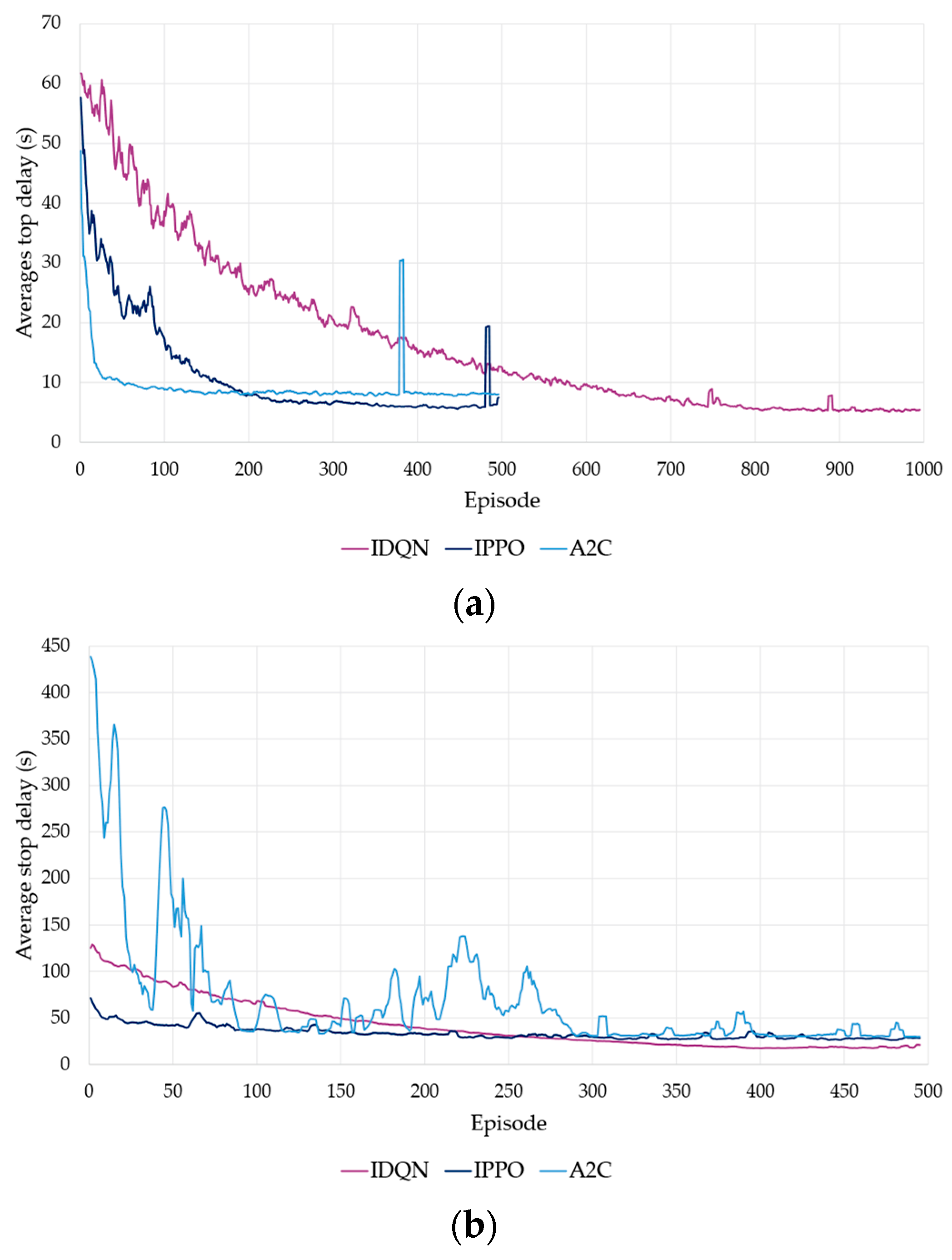
• IDQN: the independent DQN adaptive traffic signal control algorithm, in which each intersection is controlled by 1 RL agent [65];
• IPPO: the independent proximal policy optimization algorithm [65];
• A2C: the advantage actor–critic algorithm [66];
• MaxPWFlow: the MPC-based algorithm described in Section 3.2.1 [17];
• Trajectory Control: the semicooperative algorithm with MPC-based adaptive TSC control [17];
• Trajectory Control + RL: the semicooperative algorithm with IDQN-based adaptive TSC control; and
• Cooperative Control: the method of cooperative control proposed in this paper.

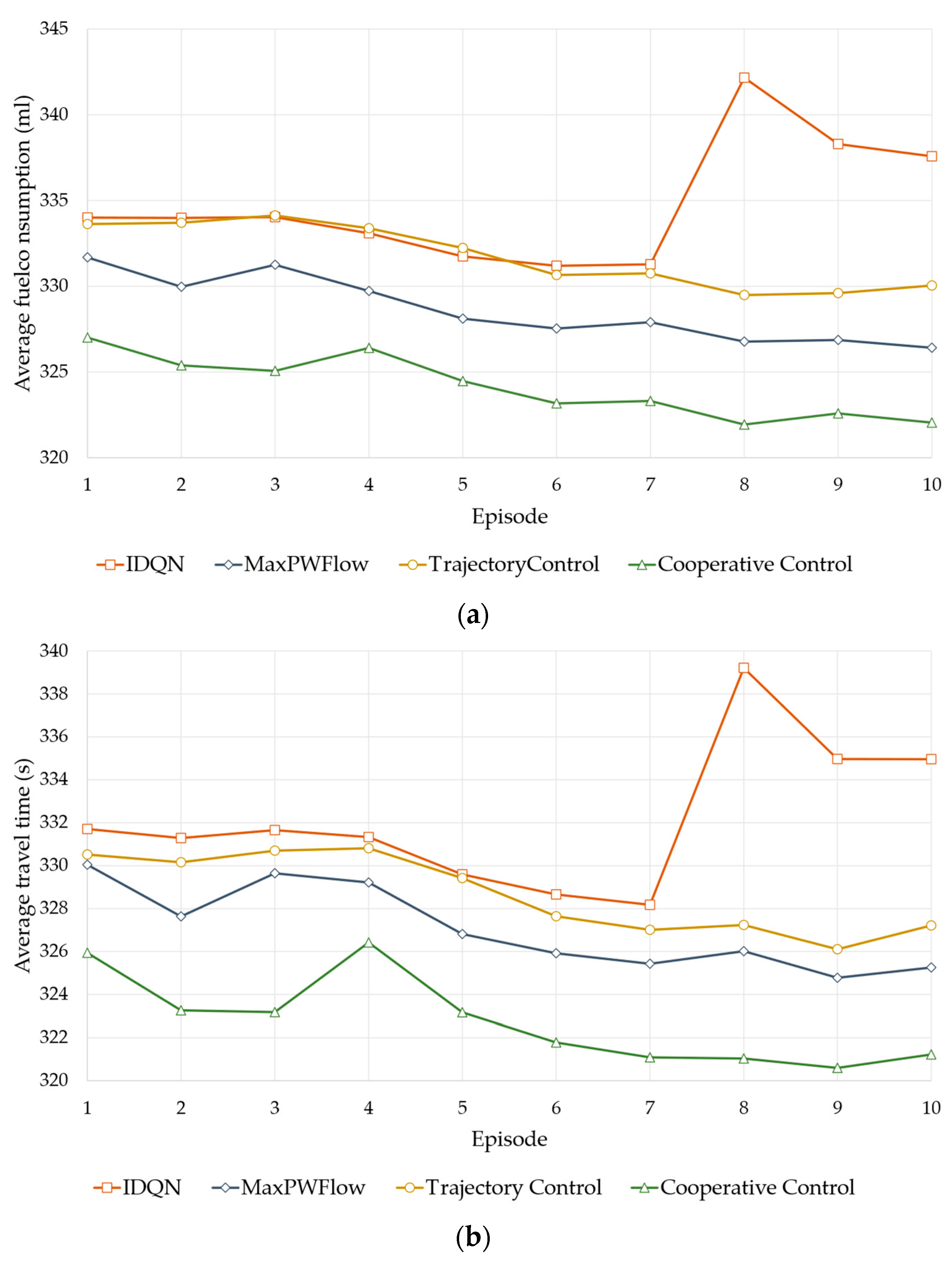
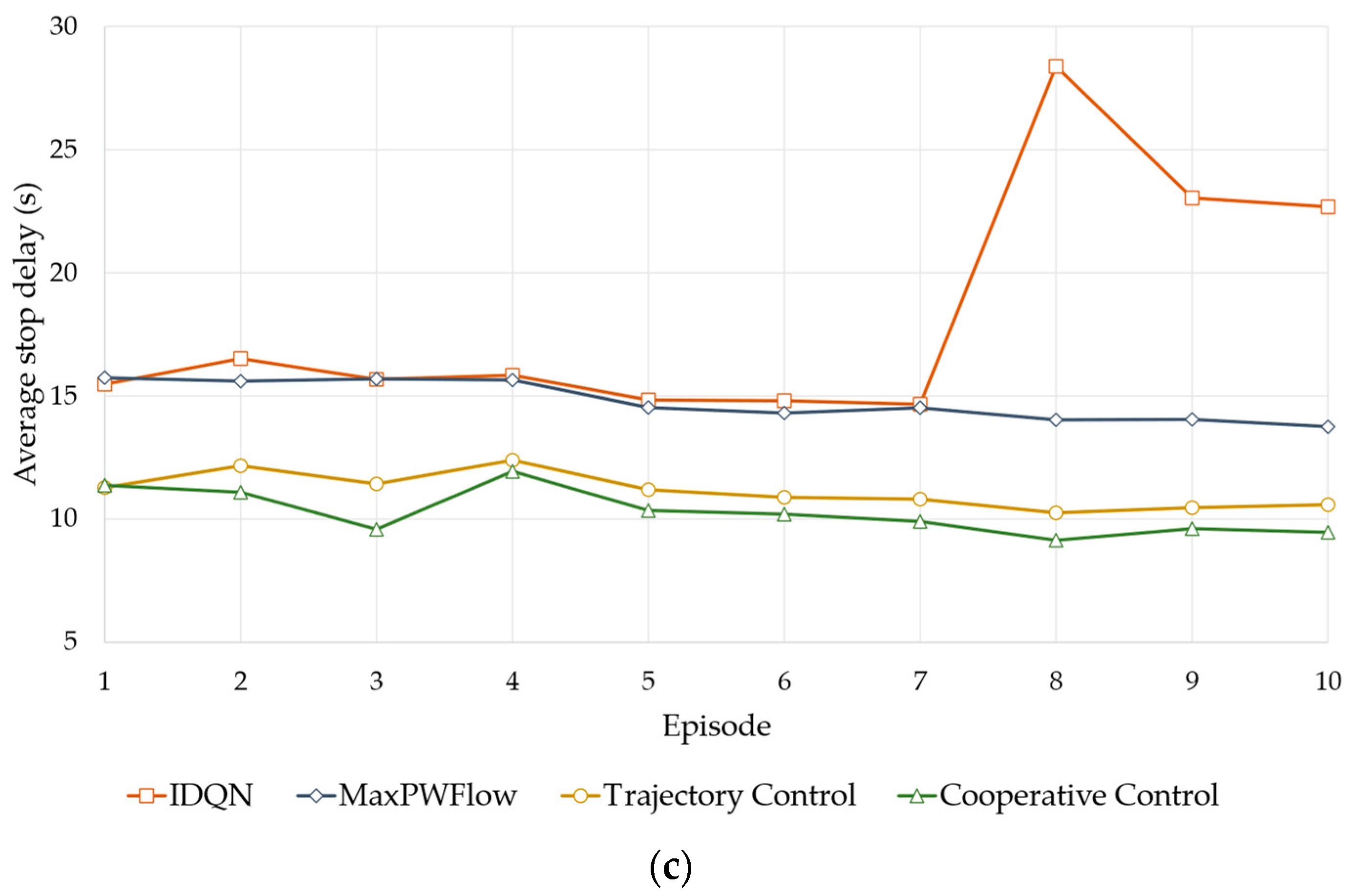
4.3. Experimental Results

In the first stage of the experimental study, we evaluated the convergence of the training process of the RL algorithms. To compare the training process, we collected the average stop delays depending on the episodes. Figure 4 shows the learning curves for each algorithm in the “Cologne-8” and “Collogne-316” scenarios. The learning curves were averaged with a sliding window over 5 episodes. According to Figure 4, the IDQN algorithm required more episodes to achieve a stable average stop delay measurement.

Table 2. Average fuel consumption (ml) for different simulation scenarios.

Model	“Cologne-3”	“Cologne-8”	“Cologne-316”
IDQN	64.24 ± 0.84	88.51 ± 1.76	334.74 ± 3.37
IPPO	64.42 ± 0.88	88.52 ± 1.74	416.93 ± 8.85
A2C	66 ± 0.6	93.68 ± 1.75	355.62 ± 9.36
MaxPWFlow	62.15 ± 0.4	86.48 ± 1.77	328.62 ± 1.81
TrajectoryControl	60.55 ± 0.46	84.42 ± 1.58	331.76 ± 1.75
Trajectory Control + RL	61.76 ± 0.43	86.52 ± 1.6	333.82 ± 1.7
Cooperative Control	59.57 ± 0.43	83.41 ± 1.5	325.25 ± 1.71

compares the average fuel consumption for each scenario. The table includes the average values and standard deviation over 10 episodes. As shown in the table, the proposed cooperative control method reduced the fuel consumption compared with the baseline methods in each scenario. The average reduction in fuel consumption ranged from 1% for the “Cologne-316” scenario to 4.2% for the “Cologne-3” scenario in comparison with noncooperative control.

In the next step, we evaluated the average travel time and average stop delays. These measurements are presented in

Table 3. Average travel time (sec) for different simulation scenarios.

Model	“Cologne-3”	“Cologne-8”	“Cologne-316”
IDQN	57.9 ± 1.08	89.89 ± 2.07	332.15 ± 3.19
IPPO	58.25 ± 1.01	89.51 ± 1.98	406.94 ± 7.92
A2C	60.57 ± 0.9	95.15 ± 2.09	350.28 ± 8.32
MaxPWFlow	55.01 ± 0.57	87.69 ± 2.03	327.08 ± 1.85
TrajectoryControl	53.48 ± 0.7	85.57 ± 1.88	328.68 ± 1.72
Trajectory Control + RL	54.5 ± 0.52	88.11 ± 1.83	331.83 ± 1.85
Cooperative Control	52.12 ± 0.44	84.32 ± 1.89	323.96 ± 1.95

and

Table 4. Average stop delays (sec) for different simulation scenarios.

Model	“Cologne-3”	“Cologne-8”	“Cologne-316”
IDQN	7.49 ± 0.82	4.46 ± 0.28	18.2 ± 4.52
IPPO	7.57 ± 0.81	4.01 ± 0.14	101.45 ± 9.24
A2C	8.9 ± 0.67	7.44 ± 0.31	29.12 ± 9.41
MaxPWFlow	6.08 ± 0.36	3.18 ± 0.15	14.79 ± 0.75
TrajectoryControl	3.65 ± 0.4	0.71 ± 0.18	11.15 ± 0.67
Trajectory Control + RL	3.27 ± 0.34	0.86 ± 0.1	12.52 ± 1.46
Cooperative Control	3.38 ± 0.37	0.62 ± 0.07	10.76 ± 0.87

, respectively.

As can be seen from the presented results, the cooperative control method showed the best results in 8 out of 9 cases. The semicooperative approach “Trajectory Control + RL” led to an insignificant reduction in the average stop delays by 0.1 s only for the “Cologne-3” scenario.

The performance measures by the average travel time criteria showed that the proposed method led to a reduction of the travel time from 1% for the “Cologne-316” scenario to 5.3% for the “Cologne-3” scenario in comparison with the MaxPWFlow algorithm. These results are similar to the average fuel consumption performance comparison. The average stop delay measurements showed that cooperative adaptive traffic signal control and trajectory optimization have the potential to reduce the stop delays by up to 27% compared to the MaxPWFlow algorithm in the “Cologne-316” large-scale scenario.

The obtained results allow us to conclude that the best result among the RL-based algorithms was shown by the value-based IDQN algorithm. However, more episodes are required to train this algorithm, as shown in Figure 4. In addition, the RL-based algorithms had a higher standard deviation, which indirectly indicated that these algorithms provided less robust results than the MPC-based TSC algorithm.

Next, we analyzed the performance measures in more detail. Figure 5 plots the considered measurements for each simulation episode of the “Cologne-316” scenario. To make the figure clearer, we show the results of the best algorithms of each type. Figure 5 shows that the proposed method performed better in each episode of the considered scenario.

Finally, we evaluated the computation time of the 2 main operations of the proposed method. The process of choosing the next phase of a traffic signal took 5 ms on average; and the construction of trajectory for 1 vehicle took 240 ms on average. The proposed method can be used in real-time processing. Additionally, it should be noted that the proposed method can be parallelized to further reduce computation time.

5. Conclusions

The development of connected and autonomous vehicles (CAVs) is the key trend in the development of intelligent transportation systems. CAVs can reduce traffic accidents, improve road safety, reduce traffic congestion, and make transport more efficient overall.

This paper proposed a method for cooperative control of traffic signals and vehicle trajectories near signalized intersections. The cooperative control method combines the adaptive traffic signal control algorithm based on maximizing the predicted weighted traffic flow and the CAVs trajectory construction algorithm.

The effectiveness of the proposed approach was experimentally evaluated in the SUMO microscopic traffic simulation package in three real-world scenarios. The results show that our method can reduce the average fuel consumption by 1% to 4.2%, the average travel time by 1% to 5.3%, and the average stop delays to 27% for different simulation scenarios compared to the best adaptive traffic signal control approach.

There are some limitations to the practical application of the proposed method. First, we assume that all vehicles in the transport network are CAVs. However, currently, the percentage of autonomous vehicles on the roads is extremely low. Second, we assume that there are no communication delays between vehicles and infrastructure, and the vehicle state information is ground truth data. Nevertheless, in reality, the exchange of information takes some time, and this information may not be accurate enough.

In future work, we plan to consider several areas of research. First, the proposed method assumes there is no communication delays between vehicles and infrastructure, which in reality is not true. Second, a comparison with other cooperative control methods is planned. Finally, an important research direction is the modification of the proposed method for application in a mixed environment with CAVs and human-driven vehicles.

References

- United States. Department of Transportation. Bureau of Transportation Statistics. Transportation Statistics Annual Report 2022; United States. Department of Transportation. Bureau of Transportation Statistics: Washington, DC, USA, 2022. [CrossRef]
- Pishue, B. 2022 INRIX Global Traffic Scorecard. Available online: https://inrix.com/scorecard/ (accessed on 18 February 2023).
- Balid, W.; Tafish, H.; Refai, H.H. Intelligent Vehicle Counting and Classification Sensor for Real-Time Traffic Surveillance. IEEE Trans. Intell. Transp. Syst. 2018, 19, 1784–1794. [Google Scholar] [CrossRef]
- Zhao, S.; Xing, S.; Mao, G. An Attention and Wavelet Based Spatial-Temporal Graph Neural Network for Traffic Flow and Speed Prediction. Mathematics 2022, 10, 3507. [Google Scholar] [CrossRef]
- Gu, Y.; Deng, L. STAGCN: Spatial–Temporal Attention Graph Convolution Network for Traffic Forecasting. Mathematics 2022, 10, 1599. [Google Scholar] [CrossRef]
- Kholodov, Y.; Alekseenko, A.; Kazorin, V.; Kurzhanskiy, A. Generalization Second Order Macroscopic Traffic Models via Relative Velocity of the Congestion Propagation. Mathematics 2021, 9, 2001. [Google Scholar] [CrossRef]
- Wei, H.; Zheng, G.; Gayah, V.; Li, Z. A Survey on Traffic Signal Control Methods. arXiv 2020, arXiv:1904.08117. [Google Scholar]
- Haydari, A.; Yılmaz, Y. Deep Reinforcement Learning for Intelligent Transportation Systems: A Survey. IEEE Trans. Intell. Transp. Syst. 2022, 23, 11–32. [Google Scholar] [CrossRef]
- Moreira-Matias, L.; Mendes-Moreira, J.; de Sousa, J.F.; Gama, J. Improving Mass Transit Operations by Using AVL-Based Systems: A Survey. IEEE Trans. Intell. Transp. Syst. 2015, 16, 1636–1653. [Google Scholar] [CrossRef]
- Sarvi, M.; Kuwahara, M. Using ITS to Improve the Capacity of Freeway Merging Sections by Transferring Freight Vehicles. IEEE Trans. Intell. Transp. Syst. 2008, 9, 580–588. [Google Scholar] [CrossRef]
- Agafonov, A.A.; Yumaganov, A.S. Bus Arrival Time Prediction Using Recurrent Neural Network with LSTM Architecture. Opt. Mem. Neural Netw. 2019, 28, 222–230. [Google Scholar] [CrossRef]
- Lv, Z.; Shang, W. Impacts of Intelligent Transportation Systems on Energy Conservation and Emission Reduction of Transport Systems: A Comprehensive Review. Green Technol. Sustain. 2023, 1, 100002. [Google Scholar] [CrossRef]
- Gupta, M.; Benson, J.; Patwa, F.; Sandhu, R. Secure V2V and V2I Communication in Intelligent Transportation Using Cloudlets. IEEE Trans. Serv. Comput. 2022, 15, 1912–1925. [Google Scholar] [CrossRef]
- Wang, Y.; Yan, Y.; Shen, T.; Bai, S.; Hu, J.; Xu, L.; Yin, G. An Event-Triggered Scheme for State Estimation of Preceding Vehicles under Connected Vehicle Environment. IEEE Trans. Intell. Veh. 2023, 8, 583–593. [Google Scholar] [CrossRef]
- Xu, B.; Ban, X.J.; Bian, Y.; Wang, J.; Li, K. V2I Based Cooperation between Traffic Signal and Approaching Automated Vehicles. In Proceedings of the 2017 IEEE Intelligent Vehicles Symposium (IV), Los Angeles, CA, USA, 11–14 June 2017. [Google Scholar]
- Agafonov, A.; Yumaganov, A.; Myasnikov, V. An Algorithm for Cooperative Control of Traffic Signals and Vehicle Trajectories. In Proceedings of the 2022 4th International Conference on Control Systems, Mathematical Modeling, Automation and Energy Efficiency (SUMMA), Lipetsk, Russia, 9–11 November 2022; pp. 675–680. [Google Scholar]
- Agafonov, A.A.; Yumaganov, A.S.; Myasnikov, V.V. Adaptive Traffic Signal Control Based on Neural Network Prediction of Weighted Traffic Flow. Optoelectron. Instrum. Data Process. 2022, 58, 503–513. [Google Scholar] [CrossRef]
- Lopez, P.A.; Wiessner, E.; Behrisch, M.; Bieker-Walz, L.; Erdmann, J.; Flotterod, Y.-P.; Hilbrich, R.; Lucken, L.; Rummel, J.; Wagner, P. Microscopic Traffic Simulation Using SUMO. In Proceedings of the 2018 21st International Conference on Intelligent Transportation Systems (ITSC), Maui, HI, USA, 4–7 November 2018; pp. 2575–2582. [Google Scholar]
- Nguyen, D.D.; Rohacs, J. Smart City Total Transport-Managing System: (A Vision Including the Cooperating, Contract-Based and Priority Transport Management). In Lecture Notes of the Institute for Computer Sciences, Social Informatics and Telecommunications Engineering; Springer International Publishing: Cham, Switzerland, 2019; pp. 74–85. ISBN 9783030058722. [Google Scholar]
- Nguyen, D.D.; Rohács, J.; Rohács, D.; Boros, A. Intelligent Total Transportation Management System for Future Smart Cities. Appl. Sci. 2020, 10, 8933. [Google Scholar] [CrossRef]
- Webster, F.V. Traffic Signal Settings; H.M. Stationery Office: Richmond, UK, 1958. [Google Scholar]
- Little, J.; Kelson, M.; Gartner, N. MAXBAND: A Program for Setting Signals on Arteries and Triangular Networks. Transp. Res. Rec. J. Transp. Res. Board 1981, 795, 40–46. [Google Scholar]
- Papageorgiou, M.; Kiakaki, C.; Dinopoulou, V.; Kotsialos, A.; Wang, Y. Review of Road Traffic Control Strategies. Proc. IEEE 2003, 91, 2043–2067. [Google Scholar] [CrossRef]
- Ribeiro, I.M.; Simões, M.d.L.d.O. The Fully Actuated Traffic Control Problem Solved by Global Optimization and Complementarity. Eng. Optim. 2016, 48, 199–212. [Google Scholar] [CrossRef]
- Cools, S.-B.; Gershenson, C.; D’Hooghe, B. Self-Organizing Traffic Lights: A Realistic Simulation. In Advances in Applied Self-Organizing Systems; Prokopenko, M., Ed.; Advanced Information and Knowledge Processing; Springer: London, UK, 2013; pp. 45–55. ISBN 978-1-4471-5113-5. [Google Scholar]
- Varaiya, P. The Max-Pressure Controller for Arbitrary Networks of Signalized Intersections. In Advances in Dynamic Network Modeling in Complex Transportation Systems; Ukkusuri, S.V., Ozbay, K., Eds.; Complex Networks and Dynamic Systems; Springer: New York, NY, USA, 2013; pp. 27–66. ISBN 978-1-4614-6243-9. [Google Scholar]
- Savithramma, R.M.; Sumathi, R. Road Traffic Signal Control and Management System: A Survey. In Proceedings of the 2020 3rd International Conference on Intelligent Sustainable Systems (ICISS), Thoothukudi, India, 3–5 December 2020; pp. 104–110. [Google Scholar]
- Lin, H.; Han, Y.; Cai, W.; Jin, B. Traffic Signal Optimization Based on Fuzzy Control and Differential Evolution Algorithm. IEEE Trans. Intell. Transp. Syst. 2022, 1–12. [Google Scholar] [CrossRef]
- Jafari, S.; Shahbazi, Z.; Byun, Y.-C. Improving the Road and Traffic Control Prediction Based on Fuzzy Logic Approach in Multiple Intersections. Mathematics 2022, 10, 2832. [Google Scholar] [CrossRef]
- Kamal, M.A.S.; Imura, J.; Ohata, A.; Hayakawa, T.; Aihara, K. Control of Traffic Signals in a Model Predictive Control Framework. IFAC Proc. Vol. 2012, 45, 221–226. [Google Scholar] [CrossRef]
- Yazici, A.; Seo, G.; Ozguner, U. A Model Predictive Control Approach for Decentralized Traffic Signal Control. IFAC Proc. Vol. 2008, 41, 13058–13063. [Google Scholar] [CrossRef]
- Nakanishi, H.; Namerikawa, T. Optimal Traffic Signal Control for Alleviation of Congestion Based on Traffic Density Prediction by Model Predictive Control. In Proceedings of the 2016 55th Annual Conference of the Society of Instrument and Control Engineers of Japan (SICE), Tsukuba, Japan, 20–23 September 2016; pp. 1273–1278. [Google Scholar]
- Shen, X.; Zhang, X.; Ouyang, T.; Li, Y.; Raksincharoensak, P. Cooperative Comfortable-Driving at Signalized Intersections for Connected and Automated Vehicles. IEEE Robot. Autom. Lett. 2020, 5, 6247–6254. [Google Scholar] [CrossRef]
- Li, L.; Wen, D.; Yao, D. A Survey of Traffic Control with Vehicular Communications. IEEE Trans. Intell. Transp. Syst. 2014, 15, 425–432. [Google Scholar] [CrossRef]
- Roess, R.; Prassas, E.; McShane, W. Traffic Engineering, 4th ed.; Pearson: Upper Saddle River, NJ, USA, 2010; ISBN 978-0-13-613573-9. [Google Scholar]
- Miao, W.; Li, L.; Wang, Z. A Survey on Deep Reinforcement Learning for Traffic Signal Control. In Proceedings of the 2021 33rd Chinese Control and Decision Conference (CCDC), Kunming, China, 22–24 May 2021; pp. 1092–1097. [Google Scholar]
- Tomar, I.; Indu, S.; Pandey, N. Traffic Signal Control Methods: Current Status, Challenges, and Emerging Trends. In Proceedings of Data Analytics and Management; Gupta, D., Polkowski, Z., Khanna, A., Bhattacharyya, S., Castillo, O., Eds.; Springer Nature: Singapore, 2022; pp. 151–163. [Google Scholar]
- Watkins, C.J.C.H.; Dayan, P. Q-Learning. Mach. Learn. 1992, 8, 279–292. [Google Scholar] [CrossRef]
- van der Pol, E.; Oliehoek, F.A. Coordinated Deep Reinforcement Learners for Traffic Light Control. In Proceedings of the Learning, Inference and Control of Multi-Agent Systems (at NIPS 2016), Barcelona, Spain, 5–10 December 2016; Available online: https://pure.uva.nl/ws/files/10793554/vanderpol_oliehoek_nipsmalic2016.pdf (accessed on 18 February 2023).
- Tan, T.; Bao, F.; Deng, Y.; Jin, A.; Dai, Q.; Wang, J. Cooperative Deep Reinforcement Learning for Large-Scale Traffic Grid Signal Control. IEEE Trans. Cybern. 2020, 50, 2687–2700. [Google Scholar] [CrossRef]
- Gao, J.; Shen, Y.; Liu, J.; Ito, M.; Shiratori, N. Adaptive Traffic Signal Control: Deep Reinforcement Learning Algorithm with Experience Replay and Target Network. arXiv 2017. [Google Scholar] [CrossRef]
- Ducrocq, R.; Farhi, N. Deep Reinforcement Q-Learning for Intelligent Traffic Signal Control with Partial Detection. Int. J. Intell. Transp. Syst. Res. 2023. [Google Scholar] [CrossRef]
- Boukerche, A.; Zhong, D.; Sun, P. A Novel Reinforcement Learning-Based Cooperative Traffic Signal System Through Max-Pressure Control. IEEE Trans. Veh. Technol. 2022, 71, 1187–1198. [Google Scholar] [CrossRef]
- van Hasselt, H.; Guez, A.; Silver, D. Deep Reinforcement Learning with Double Q-Learning. In Proceedings of the Thirtieth AAAI Conference on Artificial Intelligence; AAAI Press: Phoenix, Arizona, 2016; pp. 2094–2100. [Google Scholar]
- Agafonov, A.A.; Myasnikov, V.V. Hybrid Prediction-Based Approach for Traffic Signal Control Problem. Opt. Mem. Neural Netw. 2022, 31, 277–287. [Google Scholar] [CrossRef]
- Casas, N. Deep Deterministic Policy Gradient for Urban Traffic Light Control. arXiv 2017. [Google Scholar] [CrossRef]
- Zhu, Y.; Cai, M.; Schwarz, C.W.; Li, J.; Xiao, S. Intelligent Traffic Light via Policy-Based Deep Reinforcement Learning. Int. J. Intell. Transp. Syst. Res. 2022, 20, 734–744. [Google Scholar] [CrossRef]
- An, Y.; Zhang, J. Traffic Signal Control Method Based on Modified Proximal Policy Optimization. In Proceedings of the 2022 10th International Conference on Traffic and Logistic Engineering (ICTLE), Macau, China, 12–14 August 2022; pp. 83–88. [Google Scholar]
- Aslani, M.; Mesgari, M.S.; Seipel, S.; Wiering, M. Developing Adaptive Traffic Signal Control by Actor–Critic and Direct Exploration Methods. Proc. Inst. Civ. Eng.-Transp. 2019, 172, 289–298. [Google Scholar] [CrossRef]
- Chu, T.; Wang, J.; Codecà, L.; Li, Z. Multi-Agent Deep Reinforcement Learning for Large-Scale Traffic Signal Control. IEEE Trans. Intell. Transp. Syst. 2019, 21, 1086–1095. [Google Scholar] [CrossRef]
- Ma, D.; Zhou, B.; Song, X.; Dai, H. A Deep Reinforcement Learning Approach to Traffic Signal Control with Temporal Traffic Pattern Mining. IEEE Trans. Intell. Transp. Syst. 2022, 23, 11789–11800. [Google Scholar] [CrossRef]
- Genders, W.; Razavi, S. Evaluating Reinforcement Learning State Representations for Adaptive Traffic Signal Control. Procedia Comput. Sci. 2018, 130, 26–33. [Google Scholar] [CrossRef]
- Minnikhanov, R.; Anikin, I.; Mardanova, A.; Dagaeva, M.; Makhmutova, A.; Kadyrov, A. Evaluation of the Approach for the Identification of Trajectory Anomalies on CCTV Video from Road Intersections. Mathematics 2022, 10, 388. [Google Scholar] [CrossRef]
- Shepelev, V.; Zhankaziev, S.; Aliukov, S.; Varkentin, V.; Marusin, A.; Marusin, A.; Gritsenko, A. Forecasting the Passage Time of the Queue of Highly Automated Vehicles Based on Neural Networks in the Services of Cooperative Intelligent Transport Systems. Mathematics 2022, 10, 282. [Google Scholar] [CrossRef]
- Yu, C.; Sun, W.; Liu, H.X.; Yang, X. Managing Connected and Automated Vehicles at Isolated Intersections: From Reservation- to Optimization-Based Methods. Transp. Res. Part B Methodol. 2019, 122, 416–435. [Google Scholar] [CrossRef]
- Wang, Q.; Gong, Y.; Yang, X. Connected Automated Vehicle Trajectory Optimization along Signalized Arterial: A Decentralized Approach under Mixed Traffic Environment. Transp. Res. Part C Emerg. Technol. 2022, 145, 103918. [Google Scholar] [CrossRef]
- Zhou, F.; Li, X.; Ma, J. Parsimonious Shooting Heuristic for Trajectory Design of Connected Automated Traffic Part I: Theoretical Analysis with Generalized Time Geography. Transp. Res. Part B Methodol. 2017, 95, 394–420. [Google Scholar] [CrossRef]
- Ma, J.; Li, X.; Zhou, F.; Hu, J.; Park, B.B. Parsimonious Shooting Heuristic for Trajectory Design of Connected Automated Traffic Part II: Computational Issues and Optimization. Transp. Res. Part B Methodol. 2017, 95, 421–441. [Google Scholar] [CrossRef]
- Zhang, L.; Wang, Y.; Zhu, H. Theory and Experiment of Cooperative Control at Multi-Intersections in Intelligent Connected Vehicle Environment: Review and Perspectives. Sustainability 2022, 14, 1542. [Google Scholar] [CrossRef]
- Guo, Y.; Ma, J. DRL-TP3: A Learning and Control Framework for Signalized Intersections with Mixed Connected Automated Traffic. Transp. Res. Part C Emerg. Technol. 2021, 132, 103416. [Google Scholar] [CrossRef]
- Du, Y.; Shangguan, W.; Chai, L. A Coupled Vehicle-Signal Control Method at Signalized Intersections in Mixed Traffic Environment. IEEE Trans. Veh. Technol. 2021, 70, 2089–2100. [Google Scholar] [CrossRef]
- Tajalli, M.; Hajbabaie, A. Traffic Signal Timing and Trajectory Optimization in a Mixed Autonomy Traffic Stream. IEEE Trans. Intell. Transp. Syst. 2022, 23, 6525–6538. [Google Scholar] [CrossRef]
- HBEFA—Handbook Emission Factors for Road Transport. Available online: https://www.hbefa.net/e/index.html (accessed on 14 February 2023).
- TAPASCologne. Available online: https://sumo.dlr.de/docs/Data/Scenarios/TAPASCologne.html (accessed on 15 February 2023).
- Ault, J.; Sharon, G. Reinforcement Learning Benchmarks for Traffic Signal Control. In Proceedings of the Neural Information Processing Systems Track on Datasets and Benchmarks (Round 1), Virtual-only Conference, 6–14 December 2021; Available online: https://datasets-benchmarks-proceedings.neurips.cc/paper/2021/file/f0935e4cd5920aa6c7c996a5ee53a70f-Paper-round1.pdf (accessed on 18 February 2023).
- PFRL. Available online: https://github.com/pfnet/pfrl (accessed on 15 February 2023).