On Solutions of Fractional Integrodifferential Systems Involving Ψ-Caputo Derivative and Ψ-Riemann–Liouville Fractional Integral

Abstract

In this paper, we investigate a new class of nonlinear fractional integrodifferential systems that includes the $\Psi$-Riemann–Liouville fractional integral term. Using the technique of upper and lower solutions, the solvability of the system is examined. We add two examples to demonstrate and validate the main result. The main results highlight crucial contributions to the general theory of fractional differential equations.

1. Introduction

As of today, fractional calculus (FC), which is the generalization of derivatives and integrals to non-integer orders, has been explored and developed into a powerful indicator for finding extremely challenging hidden phenomena in dynamical systems (see [1,2,3,4,5,6,7,8,9,10,11,12,13]). There are numerous solution characterizations; however, many authors have focused on the existence of solutions to fractional differential models (see [14,15,16,17,18,19,20,21,22,23]). Recent advances in FC theory have produced significant findings in a variety of domains, including engineering, electronics, mechanics, signal processing, control theory, physics, chemistry, biology, pictures, biophysics, aerodynamics, and blood flow (see [24,25,26,27]). The fractional operators have frequently been used in numerous real-world applications (see [28,29,30,31,32]).

The FC technique is frequently applied in the context of the classical derivatives of Caputo, Riemann–Liouville, Grunwald–Letnikov, or Caputo–Hadamard. However, a new derivative operator known as the $\Psi$-Caputo fractional derivative ($\Psi$-CFD) has been presented as a generalization operator for all of the aforementioned. The benefit of the new derivative is that, by carefully choosing the psi function, all classical derivatives can be easily generated. There have been various studies looking into the qualitative characteristics of solutions for $\Psi$-fractional differential systems in recent years (see [33,34,35,36,37,38,39,40]). To demonstrate the existence theory, researchers have employed a variety of nonlinear analysis techniques, including topological degree theory, mathematical inequalities, fixed-point theory, and measure of noncompactness [41,42,43,44].

The following new nonlinear fractional differential system with the $\Psi$-Riemann–Liouville fractional integral ($\Psi$-RLFI) term will be discussed in this work.

$$\left\{\begin{array}{c}{\mathcal{D}}_{{\mathfrak{r}}_1^{+}}^{\delta ;\Psi }\varkappa \left(\varsigma \right)=\mathcal{F}\left(\varsigma ,\varkappa \left(\varsigma \right),{\mathcal{I}}_{{\mathfrak{r}}_1^{+}}^{\delta ;\Psi }\varkappa \left(\varsigma \right)\right),\varsigma \in [{\mathfrak{r}}_1,{\mathfrak{r}}_2],\hfill \\ \varkappa \left({\mathfrak{r}}_1\right)={\varkappa }_{{\mathfrak{r}}_1},\hfill \end{array}\right.$$

(1)

where ${\mathcal{D}}_{{\mathfrak{r}}_1^{+}}^{\delta ;\Psi }$ and ${\mathcal{I}}_{{\mathfrak{r}}_1^{+}}^{\delta ;\Psi }$ stand for the $\Psi$-CFD and $\Psi$-RLFI operators, which will be defined later in Definitions 2 and 4, $\mathcal{F}:[{\mathfrak{r}}_1,{\mathfrak{r}}_2]\times \mathbb{R}\times \mathbb{R}\to \mathbb{R},{\varkappa }_{{\mathfrak{r}}_1}\in \mathbb{R},$ and $0<{\mathfrak{r}}_1<{\mathfrak{r}}_2<\infty .$ The function $\Psi :[{\mathfrak{r}}_1,{\mathfrak{r}}_2]\to \mathbb{R}$ is increasing with ${\Psi }^{\prime }\left(\varsigma \right)\ne 0,$$\forall \varsigma ,$ and $\mathcal{C}(J,\mathbb{R})$ represents the Banach space of continuous functions $\varkappa :J\to \mathbb{R}$ with the norm $\parallel \varkappa \parallel =sup\left\{\right|\varkappa \left(\varsigma \right)|:\varsigma \in J\}.$

The objective of this paper is to employ the technique of upper and lower solutions (ULS) to demonstrate the existence of solutions for system (1). It should be noted that the inclusion of the $\Psi$-Riemann–Liouville fractional integral term in the main system is a unique concept that has not been considered in previous research. Many studies have looked at the usage of ULS to solve fractional boundary problems [45,46]. However, to the best of the authors’ expectations, the application of such a method for the generalized system (1) has not yet been observed.

The paper is structured as follows: Section 2 contains some fundamental definitions and crucial findings that are required in the sequential sections. Section 3 is devoted to proving the main result, which is the existence of the solutions of (1). Prior to the main theorem, system (1) is converted to an equivalent integral equation. Finally, in the last section, we present two applications to clarify the analytical validity of the results.

2. Preliminaries

Here we present some concepts and definitions that are necessary for the remaining part of the paper. Throughout the paper, we denote by $A\mathcal{C}$ the $\mathbb{R}$-valued absolutely continuous functions on $[{\mathfrak{r}}_1,{\mathfrak{r}}_2]$ and $C({\mathfrak{r}}_1,{\mathfrak{r}}_2;\mathbb{R}):=\mathcal{C}$, and $\left[\delta \right]$ indicates the integer part of the real number $\delta$.

Definition 1

([36]). Let $\varkappa :(0,\infty )\to \mathbb{R}$ be a continuous function. Then the Riemann–Liouville fractional derivative (RLFD) of order $\delta >0,n=\left[\delta \right]+1$ is defined by

$${}^{RL}{\mathcal{D}}_{0+}^{\delta }\varkappa \left(\varsigma \right)=\frac{1}{\Gamma (n-\delta )}{\left(\frac{d}{d\varsigma }\right)}^n{\int }_0^{\varsigma }{(\varsigma -\tau )}^{n-\delta -1}\varkappa \left(\tau \right)d\tau ,$$

where Γ is the Gamma function

$$\Gamma \left(\delta \right)={\int }_0^{\infty }{\varsigma }^{\delta -1}{e}^{-\varsigma }d\varsigma .$$

Definition 2

([35,39]). The Ψ-RLFI of order $\delta >0$ for a continuous function $\varkappa :\left[{\mathfrak{r}}_1,T\right]\to \mathbb{R}$ is defined by

$${\mathcal{I}}_{{\mathfrak{r}}_1^{+}}^{\delta ;\Psi }\varkappa \left(\varsigma \right)={\int }_{{\mathfrak{r}}_1}^{\varsigma }\frac{{(\Psi \left(\varsigma \right)-\Psi \left(\tau \right))}^{\delta -1}}{\Gamma \left(\delta \right)}{\Psi }^{\prime }\left(\tau \right)\varkappa \left(\tau \right)d\tau .$$

Definition 3

([35]). The CFD of order $\delta >0$ for a $\varkappa :\left[0,+\infty \right)\to \mathbb{R}$ is defined by

$${\mathcal{D}}^{\delta }\varkappa \left(\varsigma \right)=\frac{1}{\Gamma (n-\delta )}{\int }_0^{\varsigma }{\left(\varsigma -\tau \right)}^{n-\delta -1}{\varkappa }^{\left(n\right)}\left(\tau \right)d\tau ,\delta \in \left(n-1,n\right),n\in \mathbb{N}.$$

Definition 4

([35,39]). The Ψ-CFD of order $\delta >0$ for a continuous function $\varkappa :\left[{\mathfrak{r}}_1,T\right]\to \mathbb{R}$ is defined by

$${\displaystyle {\mathcal{D}}_{{\mathfrak{r}}_1^{+}}^{\delta ;\Psi }\varkappa \left(\varsigma \right)={\int }_{{\mathfrak{r}}_1}^{\varsigma }\frac{{(\Psi \left(\varsigma \right)-\Psi \left(\tau \right))}^{n-\delta -1}}{\Gamma (n-\delta )}{\Psi }^{\prime }\left(\tau \right){\partial }_{\Psi }^n\varkappa \left(\tau \right)d\tau ,\varsigma >{\mathfrak{r}}_1,\delta \in \left(n-1,n\right),}$$

where ${\partial }_{\Psi }^n={\left(\frac{1}{{\Psi }^{\prime }\left(\varsigma \right)}\frac{d}{d\varsigma }\right)}^n,n\in \mathbb{N}$.

We list some important characteristics of $\Psi$-RLFI and $\Psi$-CFD operators. The proofs can be found in [35].

Lemma 1

([35,39]). Let $q,\ell >0$, $\varkappa \in \mathcal{C}$, and $\forall \varsigma \in [{\mathfrak{r}}_1,{\mathfrak{r}}_2]$; assume $F_{{\mathfrak{r}}_1}\left(\varsigma \right)=\Psi \left(\varsigma \right)-\Psi \left({\mathfrak{r}}_1\right)$. Then

1.

${\mathcal{I}}_{{\mathfrak{r}}_1}^{q;\Psi }{\mathcal{I}}_{{\mathfrak{r}}_1}^{\ell ;\Psi }\varkappa \left(\varsigma \right)={\mathcal{I}}_{{\mathfrak{r}}_1}^{q+\ell ;\Psi }\varkappa \left(\varsigma \right),$

2.

${\mathcal{D}}_{{\mathfrak{r}}_1}^{q;\Psi }{\mathcal{I}}_{{\mathfrak{r}}_1}^{q;\Psi }\varkappa \left(\varsigma \right)=\varkappa \left(\varsigma \right),$

3.

${\displaystyle {\mathcal{I}}_{{\mathfrak{r}}_1}^{q;\Psi }{\left(F_{{\mathfrak{r}}_1}\left(\varsigma \right)\right)}^{\ell -1}=\frac{\Gamma (\ell )}{\Gamma (\ell +q)}{\left(F_{{\mathfrak{r}}_1}\left(\varsigma \right)\right)}^{\ell +q-1},}$

4.

${\displaystyle {\mathcal{D}}_{{\mathfrak{r}}_1}^{q;\Psi }{\left(F_{{\mathfrak{r}}_1}\left(\varsigma \right)\right)}^{\ell -1}=\frac{\Gamma (\ell )}{\Gamma (\ell -q)}{\left(F_{{\mathfrak{r}}_1}\left(\varsigma \right)\right)}^{\ell -q-1},}$

5.

${\mathcal{D}}_{{\mathfrak{r}}_1}^{q;\Psi }{\left(F_{{\mathfrak{r}}_1}\left(\varsigma \right)\right)}^k=0,k\in \{0,\dots ,n-1\},n\in \mathbb{N},q\in (n-1,n]$.

Lemma 2

([35,39]). Let $n-1<{\delta }_1\le n,{\delta }_2>0,{\mathfrak{r}}_1>0,\varkappa \in L({\mathfrak{r}}_1,\mathcal{T})$, and ${\mathcal{D}}_{{\mathfrak{r}}_1^{+}}^{{\delta }_1;\Psi }\varkappa \in L({\mathfrak{r}}_1,\mathcal{T})$. Then for all $\varsigma \in [{\mathfrak{r}}_1,{\mathfrak{r}}_2]$

$$\begin{array}{cc}\hfill {\mathcal{I}}_{{\mathfrak{r}}_1^{+}}^{{\delta }_1;\Psi }{\mathcal{D}}_{{\mathfrak{r}}_1^{+}}^{{\delta }_1;\Psi }\varkappa \left(\varsigma \right)& =\varkappa \left(\varsigma \right)+{\varpi }_0+{\varpi }_1\left(\Psi \left(\varsigma \right)-\Psi \left({\mathfrak{r}}_1\right)\right)+{\varpi }_2{\left(\Psi \left(\varsigma \right)-\Psi \left({\mathfrak{r}}_1\right)\right)}^2\hfill \\ \hfill & +\cdots +{\varpi }_{n-1}{\left(\Psi \left(\varsigma \right)-\Psi \left({\mathfrak{r}}_1\right)\right)}^{n-1},\hfill \end{array}$$

with ${\varpi }_{\ell }\in \mathbb{R},\ell =0,1,\dots ,n-1$. Furthermore,

$${\mathcal{D}}_{{\mathfrak{r}}_1^{+}}^{{\delta }_1;\Psi }{\mathcal{I}}_{{\mathfrak{r}}_1^{+}}^{{\delta }_1;\Psi }\varkappa \left(\varsigma \right)=\varkappa \left(\varsigma \right),$$

and

$${\mathcal{I}}_{{\mathfrak{r}}_1^{+}}^{{\delta }_1;\Psi }{\mathcal{I}}_{{\mathfrak{r}}_1^{+}}^{{\delta }_2;\Psi }\varkappa \left(\varsigma \right)={\mathcal{I}}_{{\mathfrak{r}}_1^{+}}^{{\delta }_2;\Psi }{\mathcal{I}}_{{\mathfrak{r}}_1^{+}}^{{\delta }_1;\Psi }\varkappa \left(\varsigma \right)={\mathcal{I}}_{{\mathfrak{r}}_1^{+}}^{{\delta }_1+{\delta }_2;\Psi }\varkappa \left(\varsigma \right).$$

Obviously, we can obtain

$${\mathcal{I}}_{{\mathfrak{r}}_1^{+}}^{\delta ;\Psi }{\left(\Psi \left(\varsigma \right)-\Psi \left({\mathfrak{r}}_1\right)\right)}^{\nu -1}=\frac{\Gamma \left(\nu \right)}{\Gamma (\nu +\delta )}{\left(\Psi \left(\varsigma \right)-\Psi \left({\mathfrak{r}}_1\right)\right)}^{\nu +\delta -1},$$

$${\mathcal{D}}_{{\mathfrak{r}}_1^{+}}^{\delta ;\Psi }{\left(\Psi \left(\varsigma \right)-\Psi \left({\mathfrak{r}}_1\right)\right)}^{\nu -1}=\frac{\Gamma \left(\nu \right)}{\Gamma (\nu -\delta )}{\left(\Psi \left(\varsigma \right)-\Psi \left({\mathfrak{r}}_1\right)\right)}^{\nu -\delta -1}.$$

Lemma 3

([35]). Let $\delta ,\nu$ positive real numbers.

(i) 

If $1\le \gamma <\infty$, so for $\varkappa \in L^{\gamma }({\mathfrak{r}}_1,{\mathfrak{r}}_2;\mathbb{R})$, we obtain

$${\mathcal{I}}_{{\mathfrak{r}}_1^{+}}^{\nu ;\Psi }{\mathcal{I}}_{{\mathfrak{r}}_1^{+}}^{\delta ;\Psi }\varkappa \left(\varsigma \right)={\mathcal{I}}_{{\mathfrak{r}}_1^{+}}^{\delta +\nu ;\Psi }\varkappa \left(\varsigma \right)\mathrm{for}\varsigma \in [{\mathfrak{r}}_1,{\mathfrak{r}}_2].$$

(ii) 

If $1\le \gamma <\infty$ and $\delta >\nu$, then for $\varkappa \in L^{\gamma }({\mathfrak{r}}_1,{\mathfrak{r}}_2;\mathbb{R})$, we have

$${\mathcal{D}}_{{\mathfrak{r}}_1^{+}}^{\nu ;\Psi }{\mathcal{I}}_{{\mathfrak{r}}_1^{+}}^{\delta ;\Psi }\varkappa \left(\varsigma \right)={\mathcal{I}}_{{\mathfrak{r}}_1^{+}}^{\delta -\nu ;\Psi }\varkappa \left(\varsigma \right)\mathrm{for}\varsigma \in [{\mathfrak{r}}_1,{\mathfrak{r}}_2].$$

Definition 5.

Let $0<{\mathfrak{r}}_1<{\mathfrak{r}}_2<\infty$ and $\varkappa :[{\mathfrak{r}}_1,{\mathfrak{r}}_2]\to \mathbb{R}$. The Ψ-CFD of order $\delta \in (0,1]$ of ϰ is defined by

$${\mathcal{D}}_{{\mathfrak{r}}_1^{+}}^{\delta ;\Psi }\varkappa \left(\varsigma \right)={\mathcal{D}}_{{\mathfrak{r}}_1^{+}}^{\delta ;\Psi }\left[\varkappa \left(\varsigma \right)-\varkappa \left({\mathfrak{r}}_1\right)\right]\mathrm{for}\varsigma \in [{\mathfrak{r}}_1,{\mathfrak{r}}_2].$$

Remark 1.

This shows us that if $\varkappa \in A\mathcal{C}({\mathfrak{r}}_1,{\mathfrak{r}}_2;\mathbb{R})$, then Ψ-CFD, Definition 5 has an equivalent formula

$${\mathcal{D}}_{{\mathfrak{r}}_1^{+}}^{\delta ;\Psi }\varkappa \left(\varsigma \right)=\frac{1}{\Gamma (1-\delta )}{\int }_{{\mathfrak{r}}_1}^{\varsigma }{\left(\Psi \left(\varsigma \right)-\Psi \left(\tau \right)\right)}^{-\delta }{\varkappa }^{\prime }\left(\tau \right)d\tau \mathrm{for}\varsigma \in [{\mathfrak{r}}_1,{\mathfrak{r}}_2].$$

Lemma 4

([35]). Let $\delta >0$ and $n=\left[\delta \right]+1$.

(i) 

If $\varkappa \in \mathcal{C}$, then

$${\mathcal{D}}_{{\mathfrak{r}}_1^{+}}^{\delta ;\Psi }\left({\mathcal{I}}_{{\mathfrak{r}}_1^{+}}^{\delta ;\Psi }\varkappa \left(\varsigma \right)\right)=\varkappa \left(\varsigma \right)\mathrm{for}\varsigma \in [{\mathfrak{r}}_1,{\mathfrak{r}}_2].$$

(ii) 

If $\varkappa \in A\mathcal{C}$, then

$${\mathcal{I}}_{{\mathfrak{r}}_1^{+}}^{\delta ;\Psi }\left({\mathcal{D}}_{{\mathfrak{r}}_1^{+}}^{\delta ;\Psi }\varkappa \left(\varsigma \right)\right)=\varkappa \left(\varsigma \right)-\varkappa \left({\mathfrak{r}}_1\right)\mathrm{for}\varsigma \in [{\mathfrak{r}}_1,{\mathfrak{r}}_2].$$

3. Main Results

In this section, we prove the main result, which is the existence of solutions for system (1).

Theorem 1.

Given a continuous function $\mathcal{F}:[{\mathfrak{r}}_1,{\mathfrak{r}}_2]\times \mathbb{R}\times \mathbb{R}\to \mathbb{R}$, if $\varkappa \in \mathcal{C}$ is a solution of the integral equation

$$\varkappa \left(\varsigma \right)={\varkappa }_{{\mathfrak{r}}_1}+\frac{1}{\Gamma \left(\delta \right)}{\int }_{{\mathfrak{r}}_1}^{\varsigma }{\left(\Psi \left(\varsigma \right)-\Psi \left(\tau \right)\right)}^{\delta -1}\mathcal{F}(\tau ,\varkappa \left(\tau \right),{\mathcal{I}}_{{\mathfrak{r}}_1^{+}}^{\delta }\varkappa \left(\tau \right)){\Psi }^{\prime }\left(\tau \right)d\tau \mathrm{for}\varsigma \in [{\mathfrak{r}}_1,{\mathfrak{r}}_2].$$

(2)

then it is a solution of (1).

Proof. 

Suppose that $\varkappa \in \mathcal{C}$ is a solution of (2). Obviously, we get $\varkappa \left({\mathfrak{r}}_1\right)={\varkappa }_{{\mathfrak{r}}_1}$ and $\varsigma \to {\mathcal{I}}_{{\mathfrak{r}}_1^{+}}^{\delta ;\Psi }\varkappa \left(\varsigma \right)\in \mathcal{C}$. The continuity of $\mathcal{F}$ and the integral ${\mathcal{I}}_{{\mathfrak{r}}_1^{+}}^{\delta ;\Psi }$ ensures that $\varsigma \to \mathcal{F}(\varsigma ,\varkappa \left(\varsigma \right),{\mathcal{I}}_{{\mathfrak{r}}_1^{+}}^{\delta ;\Psi }\varkappa \left(\varsigma \right))$ is continuous as well and

$${\mathcal{I}}_{{\mathfrak{r}}_1^{+}}^{\delta ;\Psi }\mathcal{F}(\varsigma ,\varkappa \left(\varsigma \right),{\mathcal{I}}_{{\mathfrak{r}}_1^{+}}^{\delta ;\Psi }\varkappa \left(\varsigma \right)){\mid }_{\varsigma ={\mathfrak{r}}_1}=0.$$

Since $\varsigma \to {\mathcal{I}}_{{\mathfrak{r}}_1^{+}}^{\delta ;\Psi }\mathcal{F}(\varsigma ,\varkappa \left(\varsigma \right),{\mathcal{I}}_{{\mathfrak{r}}_1^{+}}^{\delta ;\Psi }\varkappa \left(\varsigma \right))$ is continuous, by Equation (2) $\varkappa$ is differential for a.e. $\varsigma \in ({\mathfrak{r}}_1,{\mathfrak{r}}_2)$, i.e., $\varkappa \in A\mathcal{C}$. By Lemma 4, we obtain

$${\mathcal{D}}_{{\mathfrak{r}}_1^{+}}^{\delta ;\Psi }{\mathcal{I}}_{{\mathfrak{r}}_1^{+}}^{\delta ;\Psi }\mathcal{F}(\varsigma ,\varkappa \left(\varsigma \right),{\mathcal{I}}_{{\mathfrak{r}}_1^{+}}^{\delta ;\Psi }\varkappa \left(\varsigma \right))=\mathcal{F}(\varsigma ,\varkappa \left(\varsigma \right),{\mathcal{I}}_{{\mathfrak{r}}_1^{+}}^{\delta ;\Psi }\varkappa \left(\varsigma \right))\mathrm{for}\varsigma \in [{\mathfrak{r}}_1,{\mathfrak{r}}_2].$$

Moreover, from Remark 1 we obtain

$$\begin{array}{cc}\hfill {\mathcal{D}}_{{\mathfrak{r}}_1^{+}}^{\delta ;\Psi }[\varkappa \left(\varsigma \right)-{\varkappa }_{{\mathfrak{r}}_1}]& =\frac{1}{\Gamma (1-\delta )}{\int }_{{\mathfrak{r}}_1}^{\varsigma }{\left(\Psi \left(\varsigma \right)-\Psi \left(\tau \right)\right)}^{-\delta }{[\varkappa \left(\tau \right)-{\varkappa }_{{\mathfrak{r}}_1}]}^{\prime }d\tau \hfill \\ \hfill & =\frac{1}{\Gamma (1-\delta )}{\int }_{{\mathfrak{r}}_1}^{\varsigma }{\left(\Psi \left(\varsigma \right)-\Psi \left(\tau \right)\right)}^{-\delta }{\varkappa }^{\prime }\left(\tau \right)d\tau \hfill \\ \hfill & ={\mathcal{D}}_{{\mathfrak{r}}_1^{+}}^{\delta ;\Psi }\varkappa \left(\varsigma \right)\mathrm{for}\varsigma \in [{\mathfrak{r}}_1,{\mathfrak{r}}_2].\hfill \end{array}$$

Thus $\varkappa \in \mathcal{C}$ is a solution of (1) as desired. □

Next, we outline the ULS approach for integral Equation (2).

Definition 6.

Let $(\underline{\varkappa },\overline{\varkappa })\in \mathcal{C}\times \mathcal{C}$. We call $(\underline{\varkappa },\overline{\varkappa })$ the upper and lower solutions of (2), respectively, if

$$\underline{\varkappa }\left(\varsigma \right)\le {\varkappa }_{{\mathfrak{r}}_1}+\frac{1}{\Gamma \left(\delta \right)}{\int }_{{\mathfrak{r}}_1}^{\varsigma }{\left(\Psi \left(\varsigma \right)-\Psi \left(\tau \right)\right)}^{\delta -1}\mathcal{F}(\tau ,\underline{\varkappa }\left(\tau \right),{\mathcal{I}}_{{\mathfrak{r}}_1^{+}}^{\delta }\underline{\varkappa }\left(\tau \right)){\Psi }^{\prime }\left(\tau \right)d\tau \mathit{for}\mathit{all}\varsigma \in [{\mathfrak{r}}_1,{\mathfrak{r}}_2],$$

and

$$\overline{\varkappa }\left(\varsigma \right)\ge {\varkappa }_{{\mathfrak{r}}_1}+\frac{1}{\Gamma \left(\delta \right)}{\int }_{{\mathfrak{r}}_1}^{\varsigma }{\left(\Psi \left(\varsigma \right)-\Psi \left(\tau \right)\right)}^{\delta -1}\mathcal{F}(\tau ,\overline{\varkappa }\left(\tau \right),{\mathcal{I}}_{{\mathfrak{r}}_1^{+}}^{\delta }\overline{\varkappa }\left(\tau \right)){\Psi }^{\prime }\left(\tau \right)d\tau \mathit{for}\mathit{all}\varsigma \in [{\mathfrak{r}}_1,{\mathfrak{r}}_2].$$

For a pair $\left(\underline{\varkappa },\overline{\varkappa }\right)$ of ULS of (2), we set

$$U_{(\underline{\varkappa },\overline{\varkappa })}=\left\{\varkappa \in \mathcal{C}:\underline{\varkappa }\left(\varsigma \right)\le \varkappa \left(\varsigma \right)\le \overline{\varkappa }\left(\varsigma \right),\varsigma \in [{\mathfrak{r}}_1,{\mathfrak{r}}_2]\mathrm{and}\varkappa \mathrm{is}\mathrm{a}\mathrm{solution}\mathrm{of}\left(2\right)\right\}.$$

Theorem 2.

Suppose $\mathcal{F}\in C([{\mathfrak{r}}_1,{\mathfrak{r}}_2]\times {\mathbb{R}}^2,\mathbb{R})$. Let $\left(\underline{\varkappa },\overline{\varkappa }\right)\in \mathcal{C}\times \mathcal{C}$ be a pair of ULS of (2) with $\underline{\varkappa }\left(\varsigma \right)\le \overline{\varkappa }\left(\varsigma \right)$ for all $\varsigma \in [{\mathfrak{r}}_1,{\mathfrak{r}}_2]$. If $(\varkappa ,U)\to \mathcal{F}(\varsigma ,\varkappa ,U)$ is nondecreasing, that is

$$\mathcal{F}\left(\varsigma ,{\varkappa }_1,y_1\right)\le \mathcal{F}\left(\varsigma ,{\varkappa }_2,y_2\right)\mathit{for}{\varkappa }_1\le {\varkappa }_2\mathit{and}{y}_1\le y_2.$$

Then there exist maximal and minimal solutions ${\varkappa }_M,{\varkappa }_L\in U_{(\underline{\varkappa },\overline{\varkappa })}$, i.e., for each $\varkappa \in U_{(\underline{\varkappa },\overline{\varkappa })}$

$${\varkappa }_L\left(\varsigma \right)\le \varkappa \left(\varsigma \right)\le {\varkappa }_M\left(\varsigma \right)\mathrm{for}\mathrm{all}\varsigma \in \left[0,T\right].$$

Proof. 

We start by constructing two sequences $\left\{y_n\right\}$ and $\left\{z_n\right\}$ as follows

$$\left\{\begin{array}{c}{y}_0=\underline{\varkappa },\hfill \\ y_{n+1}\left(\varsigma \right)={\varkappa }_{{\mathfrak{r}}_1}+\frac{1}{\Gamma \left(\delta \right)}{\int }_{{\mathfrak{r}}_1}^{\varsigma }{\left(\Psi \left(\varsigma \right)-\Psi \left(\tau \right)\right)}^{\delta -1}\mathcal{F}\left(\tau ,y_n\left(\tau \right),{\mathcal{I}}_{{\mathfrak{r}}_1^{+}}^{\delta }{y}_n\left(\tau \right)\right){\Psi }^{\prime }\left(\tau \right)d\tau ,\hfill \\ \varsigma \in \left[{\mathfrak{r}}_1,{\mathfrak{r}}_2\right]\mathrm{and}n=0,1,\dots ,\hfill \end{array}\right.$$

and

$$\left\{\begin{array}{c}{z}_0=\overline{\varkappa },\hfill \\ z_{n+1}\left(\varsigma \right)={\varkappa }_{{\mathfrak{r}}_1}+\frac{1}{\Gamma \left(\delta \right)}{\int }_{{\mathfrak{r}}_1}^{\varsigma }{\left(\Psi \left(\varsigma \right)-\Psi \left(\tau \right)\right)}^{\delta -1}\mathcal{F}\left(\tau ,z_n\left(\tau \right),{\mathcal{I}}_{{\mathfrak{r}}_1^{+}}^{\delta }{z}_n\left(\tau \right)\right){\Psi }^{\prime }\left(\tau \right)d\tau ,\hfill \\ \varsigma \in \left[{\mathfrak{r}}_1,{\mathfrak{r}}_2\right]\mathrm{and}n=0,1,\dots .\hfill \end{array}\right.$$

We divide the proof into three principal steps.

Step 1. The sequences $\left\{y_n\right\}$ and $\left\{z_n\right\}$ satisfy the following relationship

$$\underline{\varkappa }\left(\varsigma \right)=y_0\left(\varsigma \right)\le y_1\left(\varsigma \right)\le y_2\left(\varsigma \right)\le \cdots \le y_n\left(\varsigma \right)\le \dots \le z_n\left(\varsigma \right)\le \dots \le z_1\left(\varsigma \right)\le z_0\left(\varsigma \right)=\overline{\varkappa }\left(\varsigma \right)$$

(3)

for $\varsigma \in [0,\mathcal{T}]$.

To begin with, we show that the sequence $\left\{y_n\right\}$ is non-decreasing and

$$y_n\left(\varsigma \right)\le z_0\left(\varsigma \right),\varsigma \in [{\mathfrak{r}}_1,{\mathfrak{r}}_2]\mathrm{for}\mathrm{all}n\in N.$$

From the hypotheses we conclude that, for all $\varsigma \in [{\mathfrak{r}}_1,{\mathfrak{r}}_2]$, we have $\underline{\varkappa }\left(\varsigma \right)=y_0\left(\varsigma \right)\le \overline{\varkappa }\left(\varsigma \right)=z_0\left(\varsigma \right)$ and

$$y_1\left(\varsigma \right)={\varkappa }_{{\mathfrak{r}}_1}+\frac{1}{\Gamma \left(\delta \right)}{\int }_{{\mathfrak{r}}_1}^{\varsigma }{\left(\Psi \left(\varsigma \right)-\Psi \left(\tau \right)\right)}^{\delta -1}\mathcal{F}(\tau ,y_0\left(\tau \right),{\mathcal{I}}_{{\mathfrak{r}}_1^{+}}^{\delta }{y}_0\left(\tau \right)){\Psi }^{\prime }\left(\tau \right)d\tau \ge y_0\left(\varsigma \right).$$

Since $(\varkappa ,U)\to \mathcal{F}(\varsigma ,\varkappa ,U)$ is non-decreasing, we have

$$\mathcal{F}\left(\tau ,y_0\left(\tau \right),{\mathcal{I}}_{{\mathfrak{r}}_1^{+}}^{\delta ;\Psi }{y}_0\left(\tau \right)\right)\le \mathcal{F}\left(\tau ,z_0\left(\tau \right),{\mathcal{I}}_{{\mathfrak{r}}_1^{+}}^{\delta ;\Psi }{z}_0\left(\tau \right)\right),$$

for $\tau \in [0,\mathcal{T}]$. This gives

$$\begin{array}{cc}\hfill y_1\left(\varsigma \right)& ={\varkappa }_{{\mathfrak{r}}_1}+\frac{1}{\Gamma \left(\delta \right)}{\int }_{{\mathfrak{r}}_1}^{\varsigma }{\left(\Psi \left(\varsigma \right)-\Psi \left(\tau \right)\right)}^{\delta -1}\mathcal{F}\left(\tau ,y_0\left(\tau \right),{\mathcal{I}}_{{\mathfrak{r}}_1^{+}}^{\delta ;\Psi }{y}_0\left(\tau \right)\right){\Psi }^{\prime }\left(\tau \right)d\tau \hfill \\ \hfill & \le {\varkappa }_{{\mathfrak{r}}_1}+\frac{1}{\Gamma \left(\delta \right)}{\int }_{{\mathfrak{r}}_1}^{\varsigma }{\left(\Psi \left(\varsigma \right)-\Psi \left(\tau \right)\right)}^{\delta -1}\mathcal{F}\left(\tau ,z_0\left(\tau \right),{\mathcal{I}}_{{\mathfrak{r}}_1^{+}}^{\delta ;\Psi }{z}_0\left(\tau \right)\right){\Psi }^{\prime }\left(\tau \right)d\tau \le z_0\left(\varsigma \right)\mathrm{for}\varsigma \in [{\mathfrak{r}}_1,{\mathfrak{r}}_2].\hfill \end{array}$$

Therefore, we assume inductively that

$$y_{n-1}\left(\varsigma \right)\le y_n\left(\varsigma \right)\le z_0\left(\varsigma \right)\mathrm{for}\varsigma \in [{\mathfrak{r}}_1,{\mathfrak{r}}_2].$$

By virtue of the definition of $\left\{y_n\right\}$, we have

$$\begin{array}{cc}\hfill y_n\left(\varsigma \right)& ={\varkappa }_{{\mathfrak{r}}_1}+\frac{1}{\Gamma \left(\delta \right)}{\int }_{{\mathfrak{r}}_1}^{\varsigma }{\left(\Psi \left(\varsigma \right)-\Psi \left(\tau \right)\right)}^{\delta -1}\mathcal{F}(\tau ,y_{n-1}\left(\tau \right),{\mathcal{I}}_{{\mathfrak{r}}_1^{+}}^{\delta ;\Psi }{y}_{n-1}\left(\tau \right)){\Psi }^{\prime }\left(\tau \right)d\tau ,\hfill \\ \hfill y_{n+1}\left(\varsigma \right)& ={\varkappa }_{{\mathfrak{r}}_1}+\frac{1}{\Gamma \left(\delta \right)}{\int }_{{\mathfrak{r}}_1}^{\varsigma }{\left(\Psi \left(\varsigma \right)-\Psi \left(\tau \right)\right)}^{\delta -1}\mathcal{F}(\tau ,y_n\left(\tau \right),{\mathcal{I}}_{{\mathfrak{r}}_1^{+}}^{\delta ;\Psi }{y}_n\left(\tau \right)){\Psi }^{\prime }\left(\tau \right)d\tau ,\hfill \end{array}$$

for $\varsigma \in [0,\mathcal{T}]$. Since $\mathcal{F}$ is monotonous, we easily get

$$y_n\left(\varsigma \right)\le y_{n+1}\left(\varsigma \right)\le z_0\left(\varsigma \right)\mathrm{for}\varsigma \in [{\mathfrak{r}}_1,{\mathfrak{r}}_2].$$

Moreover, we have

$$y_n\left(\varsigma \right)\le z_n\left(\varsigma \right)\mathrm{for}\varsigma \in [{\mathfrak{r}}_1,{\mathfrak{r}}_2]\mathrm{and}n\in N.$$

Indeed, we get $\underline{\varkappa }\left(\varsigma \right)=y_0\left(\varsigma \right)\le z_0\left(\varsigma \right)=\overline{\varkappa }\left(\varsigma \right)$ for $n=0$. Inductively we assume

$$y_n\left(\varsigma \right)\le z_n\left(\varsigma \right),\varsigma \in [{\mathfrak{r}}_1,{\mathfrak{r}}_2].$$

Similarly, we obtain from the monotony of $\mathcal{F}$ with respect to the second and third arguments that

$$y_{n+1}\left(\varsigma \right)\le z_{n+1}\left(\varsigma \right),\varsigma \in [{\mathfrak{r}}_1,{\mathfrak{r}}_2].$$

Further, it is clear that the sequence $\left\{z_n\right\}$ is nonincreasing.

Step 2. $\left\{y_n\right\}$ and $\left\{z_n\right\}$ are relatively compact in $\mathcal{C}$.

Since $\mathcal{F}$ is continuous and $\underline{\varkappa },\overline{\varkappa }\in \mathcal{C}$, based on Step 1, $\left\{y_n\right\}$ and $\left\{z_n\right\}$ belong to $\mathcal{C}$. Then, by (3), we conclude that $\left\{y_n\right\}$ and $\left\{z_n\right\}$ are uniformly bounded. Additionally, for any ${\varsigma }_1,{\varsigma }_2\in [{\mathfrak{r}}_1,{\mathfrak{r}}_2]$ with ${\varsigma }_1\le {\varsigma }_2$, we have

$$\begin{array}{cc}\hfill & \left|y_{n+1}\left({\varsigma }_1\right)-y_{n+1}\left({\varsigma }_2\right)\right|\hfill \\ \hfill & =\frac{1}{\Gamma \left(\delta \right)}\left|{\int }_{{\mathfrak{r}}_1}^{{\varsigma }_2}{\left(\Psi \left({\varsigma }_2\right)-\Psi \left(\tau \right)\right)}^{\delta -1}\mathcal{F}(\tau ,y_n\left(\tau \right),{\mathcal{I}}_{{\mathfrak{r}}_1^{+}}^{\delta ;\Psi }{y}_n\left(\tau \right)){\Psi }^{\prime }\left(\tau \right)d\tau \right.\hfill \\ \hfill & -\left.{\int }_{{\mathfrak{r}}_1}^{{\varsigma }_1}{\left(\Psi \left({\varsigma }_1\right)-\Psi \left(\tau \right)\right)}^{\delta -1}\mathcal{F}(\tau ,y_n\left(\tau \right),{\mathcal{I}}_{{\mathfrak{r}}_1^{+}}^{\delta ;\Psi }{y}_n\left(\tau \right)){\Psi }^{\prime }\left(\tau \right)d\tau \right|\hfill \\ \hfill & =\frac{1}{\Gamma \left(\delta \right)}\left|{\int }_{{\mathfrak{r}}_1}^{{\varsigma }_2}\left[{\left(\Psi \left({\varsigma }_2\right)-\Psi \left(\tau \right)\right)}^{\delta -1}-{\left(\Psi \left({\varsigma }_1\right)-\Psi \left(\tau \right)\right)}^{\delta -1}\right]\mathcal{F}(\tau ,y_n\left(\tau \right),{\mathcal{I}}_{{\mathfrak{r}}_1^{+}}^{\delta ;\Psi }{y}_n\left(\tau \right)){\Psi }^{\prime }\left(\tau \right)d\tau \right.\hfill \\ \hfill & +\left.{\int }_{{\varsigma }_1}^{{\varsigma }_2}{\left(\Psi \left({\varsigma }_2\right)-\Psi \left(\tau \right)\right)}^{\delta -1}\mathcal{F}(\tau ,y_n\left(\tau \right),{\mathcal{I}}_{{\mathfrak{r}}_1^{+}}^{\delta ;\Psi }{y}_n\left(\tau \right)){\Psi }^{\prime }\left(\tau \right)d\tau \right|\hfill \\ \hfill & \le \frac{M}{\Gamma \left(\delta \right)}\left|{\int }_{{\mathfrak{r}}_1}^{{\varsigma }_1}\left[{\left(\Psi \left({\varsigma }_2\right)-\Psi \left(\tau \right)\right)}^{\delta -1}-{\left(\Psi \left({\varsigma }_1\right)-\Psi \left(\tau \right)\right)}^{\delta -1}\right]{\Psi }^{\prime }\left(\tau \right)d\tau \right.\hfill \\ \hfill & +\left.{\int }_{{\varsigma }_1}^{{\varsigma }_2}{\left(\Psi \left({\varsigma }_2\right)-\Psi \left(\tau \right)\right)}^{\delta -1}{\Psi }^{\prime }\left(\tau \right)d\tau \right|\hfill \\ \hfill & \le \frac{M}{\Gamma (1+\delta )}\left[2{\left(\Psi \left({\varsigma }_2\right)-\Psi \left({\varsigma }_1\right)\right)}^{\delta }\right]\to 0,\mathrm{as}\left|{\varsigma }_1-{\varsigma }_2\right|\to 0,\hfill \end{array}$$

where $M>0$. Hence $\left\{y_n\right\}$ is equicontinuous in $\mathcal{C}$.

By utilizing the Arzelà–Ascoli Theorem (see [47]), we see that $\left\{y_n\right\}$ is relatively compact in $\mathcal{C}$. Similarly $\left\{z_n\right\}$ is relatively compact in $\mathcal{C}$.

Step 3. The existence of ${\varkappa }_M,{\varkappa }_L$ in $U_{\left(\underline{\varkappa },\overline{\varkappa }\right)}$.

Since the sequences $\left\{y_n\right\}$ and $\left\{z_n\right\}$ are monotone and relatively compact in $\mathcal{C}$, there exist continuous functions y and z with $y_n\left(\varsigma \right)\le y\left(\varsigma \right)\le z\left(\varsigma \right)\le z_n\left(\varsigma \right)$, $\forall \varsigma \in [{\mathfrak{r}}_1,{\mathfrak{r}}_2]$ and $n\in N$, such that $\left\{y_n\right\}$ and $\left\{z_n\right\}$, respectively, converge uniformly to y and z in $\mathcal{C}$. Hence, y and z are solutions of the integral Equation (2), i.e.,

$$y\left(\varsigma \right)={\varkappa }_{{\mathfrak{r}}_1}+\frac{1}{\Gamma \left(\delta \right)}{\int }_{{\mathfrak{r}}_1}^{\varsigma }{\left(\Psi \left(\varsigma \right)-\Psi \left(\tau \right)\right)}^{\delta -1}\mathcal{F}(\tau ,y\left(\tau \right),{\mathcal{I}}_{{\mathfrak{r}}_1^{+}}^{\delta ;\Psi }y\left(\tau \right)){\Psi }^{\prime }\left(\tau \right)d\tau ,$$

$$z\left(\varsigma \right)={\varkappa }_{{\mathfrak{r}}_1}+\frac{1}{\Gamma \left(\delta \right)}{\int }_{{\mathfrak{r}}_1}^{\varsigma }{\left(\Psi \left(\varsigma \right)-\Psi \left(\tau \right)\right)}^{\delta -1}\mathcal{F}(\tau ,z\left(\tau \right),{\mathcal{I}}_{{\mathfrak{r}}_1^{+}}^{\delta ;\Psi }z\left(\tau \right)){\Psi }^{\prime }\left(\tau \right)d\tau ,$$

for $\varsigma \in [{\mathfrak{r}}_1,{\mathfrak{r}}_2]$. From (3) we have

$$\underline{\varkappa }\left(\varsigma \right)\le y\left(\varsigma \right)\le z\left(\varsigma \right)\le \overline{\varkappa }\left(\varsigma \right)\mathrm{for}\varsigma \in [{\mathfrak{r}}_1,{\mathfrak{r}}_2].$$

We conclude by showing that y and z are the minimum and maximum solutions in $U_{(\underline{\varkappa },\overline{\varkappa })}$. Let $\varkappa \in U_{(\underline{\varkappa },\overline{\varkappa })}$. Knowing that $\mathcal{F}$ is non-decreasing with respect to the second and third variables, we obtain

$$\underline{\varkappa }\left(\varsigma \right)\le y_n\left(\varsigma \right)\le \varkappa \left(\varsigma \right)\le z_n\left(\varsigma \right)\le \overline{\varkappa }\left(\varsigma \right)\mathrm{for}\varsigma \in [{\mathfrak{r}}_1,{\mathfrak{r}}_2]\mathrm{and}n\in N.$$

By taking $n\to \infty$, we get

$$\underline{\varkappa }\left(\varsigma \right)\le y\left(\varsigma \right)\le \varkappa \left(\varsigma \right)\le z\left(\varsigma \right)\le \overline{\varkappa }\left(\varsigma \right)\mathrm{for}\varsigma \in [{\mathfrak{r}}_1,{\mathfrak{r}}_2].$$

This implies that ${\varkappa }_L=y$ and ${\varkappa }_M=z$ are, respectively, the minimal and the maximal solution in $U_{(\underline{\varkappa },\overline{\varkappa })}$, as desired. □

Theorem 3.

If the the assumptions of Theorem 2 hold then (1) admits at least one solution in $\mathcal{C}$.

Proof. 

From Theorem 2, we get $U_{(\underline{\varkappa },\overline{\varkappa })}\ne \varnothing$, i.e., the solution set of the integral Equation (2) is a nonempty set in $\mathcal{C}$. Combining this with the result of Theorem 1 implies that (1) accepts at least one solution in $\mathcal{C}$; the proof is finished. □

4. Applications

We discuss here two concrete examples to illustrate the above results. In short, we consider a particular case for the $\Psi$-Caputo sense, which is the Caputo–Hadamard operator. That is, $\Psi \left(\varsigma \right)=ln\varsigma$.

Example 1.

Consider the following Ψ-Caputo fractional differential equation

$$\left\{\begin{array}{c}{\mathcal{D}}_{1+}^{\frac{1}{5}}\varkappa \left(\varsigma \right)=\frac{37}{20\sqrt{\pi }}{\left(ln\varsigma \right)}^{\frac{3}{5}}+\varkappa \left(\varsigma \right)\mathit{for}\varsigma \in [1,e],\hfill \\ \varkappa \left(1\right)=0.\hfill \end{array}\right.$$

(4)

Let $\mathcal{F}$ be defined as $\mathcal{F}\left(\varsigma ,\varkappa \left(\varsigma \right)\right)=\frac{37}{20\sqrt{\pi }}\left({\left(ln\varsigma \right)}^{\frac{3}{5}}+\varkappa \left(\varsigma \right)\right)$ for $\varsigma \in [1,e]$. In view of Theorem 1, we just need to show that the following fractional integral equation accepts at least one solution in $\mathcal{C}$,

$$\varkappa \left(\varsigma \right)={\mathcal{I}}_{1+}^{\frac{1}{5}}\left(\frac{37}{20\sqrt{\pi }}{\left(ln\varsigma \right)}^{\frac{3}{5}}+\varkappa \left(\varsigma \right)\right)\mathrm{for}\varsigma \in [1,e].$$

(5)

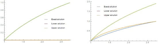
Indeed, we can see that $\left(\underline{\varkappa }\left(\varsigma \right),\overline{\varkappa }\left(\varsigma \right)\right)=\left(0,ln\varsigma \right)$ is a pair of ULS of (5). In addition, $\mathcal{F}$ is a continuous and non-decreasing function with respect to the second variable. We evaluate the sequences $\left\{y_n\right\}$ and $\left\{z_n\right\}$ by

$$\begin{gathered} \left\{\begin{array}{c}{y}_0\left(\varsigma \right)=\underline{\varkappa }\left(\varsigma \right),\hfill \\ y_{n+1}\left(\varsigma \right)={\mathcal{I}}_{1+}^{\frac{1}{5}}\mathcal{F}\left({\varsigma }_{,}{y}_n\left(\varsigma \right)\right),n=0,1,\dots ,\hfill \end{array}\right. \\ \left\{\begin{array}{c}{z}_0\left(\varsigma \right)=\overline{\varkappa }\left(\varsigma \right),\hfill \\ z_{n+1}\left(\varsigma \right)={\mathcal{I}}_{1+}^{\frac{1}{5}}\mathcal{F}\left({\varsigma }_{,}{z}_n\left(\varsigma \right)\right),n=0,1,\dots ,\hfill \end{array}\right. \end{gathered}$$

(6)

for $\varsigma \in [1,e]$. We can now dispense with Theorem 2 to obtain $y_n\to y$ and $z_n\to z$ with y and $z\in \mathcal{C}$ as $n\to \infty$. Thus, we can come up with $z\left(\varsigma \right)=y\left(\varsigma \right)=ln\varsigma$ for $\varsigma \in [1,e]$. The approximation of sequences $\left\{y_n\right\}$ and $\left\{z_n\right\}$ to $ln\varsigma$ is visible in Figure 1.

Example 2.

Consider the following Ψ-Caputo fractional differential equation

$$\left\{\begin{array}{c}{\mathcal{D}}_{1+}^{\frac{1}{2}}\varkappa \left(\varsigma \right)=\frac{16}{5\sqrt{\pi }}{(ln\varsigma )}^{\frac{5}{2}}-\frac{183}{50\sqrt{\pi }}{(ln\varsigma )}^{\frac{7}{2}}+{\mathcal{I}}_{1+}^{\frac{1}{2}}\varkappa \left(\varsigma \right)\mathrm{for}\varsigma \in [1,e],\hfill \\ \varkappa \left(1\right)=0.\hfill \end{array}\right.$$

(7)

Let $\mathcal{F}$ be defined as $\mathcal{F}$$(\varsigma ,\varkappa \left(\varsigma \right),I_{+}^{\frac{1}{2}}\varkappa \left(\varsigma \right))=\frac{16}{5\sqrt{\pi }}{(ln\varsigma )}^{\frac{5}{2}}-\frac{183}{50\sqrt{\pi }}{(ln\varsigma )}^{\frac{7}{2}}+{\mathcal{I}}_{1+}^{\frac{1}{2}}\varkappa \left(\varsigma \right)$ for $\varsigma \in [1,e]$. Hence, the corresponding fractional integral equation is given by

$$\varkappa \left(\varsigma \right)={\mathcal{I}}_{+}^{\frac{1}{2}}\left(\frac{16}{5\sqrt{\pi }}{(ln\varsigma )}^{\frac{5}{2}}-\frac{183}{50\sqrt{\pi }}{(ln\varsigma )}^{\frac{7}{2}}+{\mathcal{I}}_{1+}^{\frac{1}{2}}\varkappa \left(\varsigma \right)\right)\mathrm{for}\varsigma \in [1,e].$$

(8)

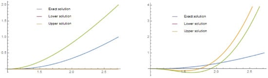
Clearly, $(\underline{\varkappa }\left(\varsigma \right),\overline{\varkappa }\left(\varsigma \right))=(0,{(ln\varsigma )}^3+{(ln\varsigma )}^4)$ is a pair of ULS of (8). All assumptions of Theorem 2 are met. Therefore, we provide sequences $\left\{y_n\right\}$ and $\left\{z_n\right\}$ by

$$\left\{\begin{array}{c}{y}_0\left(\varsigma \right)=\underline{\varkappa }\left(\varsigma \right),\hfill \\ y_{n+1}\left(\varsigma \right)={\mathcal{I}}_{1+}^{\frac{1}{2}}\mathcal{F}\left(\varsigma ,y_n\left(\varsigma \right),{\mathcal{I}}_{1+}^{\frac{1}{2}}{y}_n\left(\varsigma \right)\right),n=0,1,\dots ,\hfill \end{array}\right.$$

and

$$\left\{\begin{array}{c}{z}_0\left(\varsigma \right)=\overline{\varkappa }\left(\varsigma \right),\hfill \\ z_{n+1}\left(\varsigma \right)={\mathcal{I}}_{1+}^{\frac{1}{2}}\mathcal{F}\left(\varsigma ,z_n\left(\varsigma \right),{\mathcal{I}}_{1+}^{\frac{1}{2}}{z}_n\left(\varsigma \right)\right),n=0,1,\dots \hfill \end{array}\right.$$

Based on Theorem 2, we get $\left\{y_n\right\}$ and $y_n\to y\in \mathcal{C}$ and $z_n\to z\in \mathcal{C}$ as $n\to \infty$. Further, we can come up with $z\left(\varsigma \right)=y\left(\varsigma \right)={\left(ln\varsigma \right)}^3$ for $\varsigma \in [1,e]$. Moreover, we can also get the approximation results, Figure 2.

Remark 2.

To further grasp the benefit of taking system (1) into consideration, it is important to note that none of the prior results may be used to make any judgments about the existence of solutions of Equation (4) or Equation (7).

5. Conclusions

In this research, we applied the upper and lower solution technique to get unique and qualitative conclusions for a novel class of nonlinear integrodifferential systems. We took into account the $psi$-Caputo fractional derivative equation in a broad context that also includes the $psi$-Riemann–Liouville fractional integral term, demonstrating the existence of a solution. Two real-world examples have been used to bolster our theoretical research. The primary findings emphasize important contributions to the general theory of fractional differential equations.

References

- Baleanu, D.; Diethelm, K.; Scalas, E.; Trujillo, J.I. Fractional Calculus, Models and Numerical Methods; Series on Complexity, Nonlinearity and Chaos; World Scientific Publishing Co., Pte. Ltd.: Hackensack, NJ, USA, 2012. [Google Scholar]
- Chen, F.-L.; Zhou, Y. Attractivity fractional functional differential equations. Comput. Math. Appl. 2011, 62, 1359–1369. [Google Scholar] [CrossRef]
- Hilfer, R. (Ed.) Applications of Fractional Calculus in Physics; World Scientific Publishing Co., Inc.: River Edge, NJ, USA, 2000. [Google Scholar]
- Shatanawi, W.; Boutiara, A.; Abdo, M.S.; Jeelani, M.B.; Abodayeh, K. Nonlocal and multiple-point fractional boundary value problem in the frame of a generalized Hilfer derivative. Adv. Differ. Equ. 2021, 2021, 294. [Google Scholar] [CrossRef]
- Magin, R.L. Fractional Calculus in Bioengineering; Begell House: Redding, CT, USA, 2006. [Google Scholar]
- Shah, K.; Khan, R.A. Existence and uniqueness results to a coupled system of fractional order boundary value problems by topological degree theory. Numer. Funct. Anal. Optim. 2016, 37, 887–899. [Google Scholar] [CrossRef]
- Khan, H.; Gómez-Aguilar, J.F.; Alkhazzan, A.; Khan, A. A fractional order HIV-TB coinfection model with nonsingular Mittag-Leffler Law. Math. Methods Appl. Sci. 2020, 43, 3786–3806. [Google Scholar] [CrossRef]
- Mainardi, F. Fractional Calculus and Waves in Linear Viscoelasticity, An Introduction to Mathematical Models; Imperial College Press: London, UK, 2010. [Google Scholar]
- Podlubny, I. Fractional differential equations, An introduction to fractional derivatives, fractional differential equations, to methods of their solution and some of their applications. In Mathematics in Science and Engineering; Academic Press, Inc.: San Diego, CA, USA, 1999. [Google Scholar]
- Zada, A.; Waheed, H.; Alzabut, J.; Wang, X. Existence and stability of impulsive coupled system of fractional integrodifferential equations. Demonstr. Math. 2019, 52, 296–335. [Google Scholar] [CrossRef]
- Yang, X.-J. A new integral transform operator for solving the heat-diffusion problem. Appl. Math. Lett. 2017, 64, 193–197. [Google Scholar] [CrossRef]
- Yang, X.-J.; Baleanu, D.; Srivastava, H.M. Localfractional Integral Transforms and Their Applications; Elsevier/Academic Press: Amsterdam, The Netherlands, 2016. [Google Scholar]
- Yang, X.-J.; Machado, J.A.T. A new fractional operator of variable order: Application in the description of anomalous diffusion. Phys. A 2017, 418, 276–283. [Google Scholar] [CrossRef]
- Matar, M.M.; Amra, I.A.; Alzabut, J. Existence of solutions for tripled system of fractional differential equations involving cyclic permutation boundary conditions. Bound. Value Probl. 2020, 2020, 140. [Google Scholar] [CrossRef]
- Boulares, H.; Ardjouni, A.; Laskri, Y. Existence and uniqueness of solutions for nonlinear fractional nabla difference systems with initial conditions. Fract. Differ. Calc. 2017, 7, 247–263. [Google Scholar] [CrossRef]
- Hallaci, A.; Boulares, H.; Ardjouni, A. Existence and uniqueness for delay fractional differential equations with mixed fractional derivatives. Open J. Math. Anal. 2020, 4, 26–31. [Google Scholar] [CrossRef]
- Hallaci, A.; Boulares, H.; Kurulay, M. On the Study of Nonlinear Fractional Differential Equations on Unbounded Interval. Gen. Lett. Math. 2018, 5, 111–117. [Google Scholar] [CrossRef]
- Boulares, H.; Ardjouni, A.; Laskri, Y. Existence and Uniqueness of Solutions to Fractional Order Nonlinear Neutral Differential Equations. Appl. Math. E-Notes 2018, 18, 25–33. Available online: http://www.math.nthu.edu.tw/amen/ (accessed on 30 December 2022).
- Biroud, K. Nonlocal fractional system involving the fractional p,q-Laplacians and singular potentials. Arab. J. Math. 2022, 11, 497–505. [Google Scholar] [CrossRef]
- Mukherjee, T.; Sreenadh, K. On Dirichlet problem for fractional p-Laplacian with singular non-linearity. Adv. Nonlinear Anal. 2019, 8, 52–72. [Google Scholar] [CrossRef]
- Mazón, J.M.; Rossi, J.D.; Toledo, J. Fractional p-Laplacian evolution equations. J. Math. Pures Appl. 2016, 105, 810–844. [Google Scholar] [CrossRef]
- Razani, A.; Behboudi, F. Weak solutions for some fractional singular (p; q)-Laplacian nonlocal problems with Hardy potential. Rend. Circ. Mat. Palermo Ser. 2022, 2, 1–16. [Google Scholar] [CrossRef]
- Abdolrazaghi, F.; Razani, A. A unique weak solution for a kind of coupled system of fractional Schrodinger equations. Opusc. Math. 2020, 40, 313–322. [Google Scholar] [CrossRef]
- Zeng, F.-H.; Li, C.-P.; Liu, F.-W.; Turner, I. The use of finite difference element approaches for solving the time-fractional subdiffusion equation. SIAM J. Sci. Comput. 2013, 35, 2976–3000. [Google Scholar] [CrossRef]
- Zhang, Y.-N.; Sun, Z.-Z.; Zhao, X. Compact alternating direction implicit scheme for the two-dimensional fractional diffusion-wave equation. SIAM J. Numer. Anal. 2012, 50, 1535–1555. [Google Scholar] [CrossRef]
- Alzabut, J.; Selvam, A.G.M.; El-Nabulsi, R.A.; Vignesh, D.; Samei, M.E. Asymptotic Stability of Nonlinear Discrete Fractional Pantograph Equations with Non-Local Initial Conditions. Symmetry 2021, 13, 473. [Google Scholar] [CrossRef]
- Zhao, X.; Sun, Z.-Z. A box-type scheme fractional sub-diffusion equation with Neumann boundary conditions. J. Comput. Phys. 2011, 230, 6061–6074. [Google Scholar] [CrossRef]
- Chen, W.; Sun, H.-G.; Zhang, X.-D.; Korošak, D. Anomalous diffusion modeling by fractal and fractional derivatives. Comput. Math. Appl. 2010, 59, 1754–1758. [Google Scholar] [CrossRef]
- Chen, R.; Zhou, S.-M. Well-posedness and persistence properties for two-component higher order Camassa-Holm systems with fractional inertia operator. Nonlinear Anal. Real World Appl. 2017, 33, 121–138. [Google Scholar] [CrossRef]
- Fiscella, A.; Pucci, P. p-fractional Kirchhoff equations involving critical nonlinearities. Nonlinear Anal. Real World Appl. 2017, 35, 350–378. [Google Scholar] [CrossRef]
- Sun, H.-G.; Chen, W.; Li, C.-P.; Chen, Y.-Q. Finite difference schemes for variable-order time fractional diffusion equation. Int. J. Bifurc. Chaos Appl. Sci. Eng. 2012, 22, 1250085. [Google Scholar] [CrossRef]
- Sun, H.-G.; Chen, W.; Wei, H.; Chen, Y.-Q. A comparative study of constant-order and variable-order fractional models in characterizing memory property of systems. Eur. Phys. J. 2011, 193, 185–192. [Google Scholar] [CrossRef]
- Butzer, P.L.; Kilbas, A.A.; Trujillo, J.I. Fractional calculus in the Mellin setting and Hadamard-type fractional integrals. J. Math. Anal. Appl. 2002, 269, 1–27. [Google Scholar] [CrossRef]
- Gambo, Y.Y.; Jarad, F.; Baleanu, D.; Abdeljawad, T. On Caputo modification of the Hadamard fractional derivatives. Adv. Differ. Equ. 2014, 2014, 1–12. [Google Scholar] [CrossRef]
- Samko, S.G.; Kilbas, A.A.; Marichev, O.I. Fractional Integrals and Derivatives: Theory and Applications; Gordon and Breach Science: Yverdon, Switzerland, 1993. [Google Scholar]
- Kilbas, A.A.; Srivastava, H.M.; Trujillo, J.J. Theory and Applications Fractional Differential Equations; North-Holland Mathematics Studies; Elsevier Science B.V.: Amsterdam, The Netherlands, 2006. [Google Scholar]
- Pan, N.; Zhang, B.-L.; Cao, J. Degenerate Kirchhoff-type diffusion problems involving the fractional p-Laplacian. Nonlinear Anal. Real World Appl. 2017, 37, 56–70. [Google Scholar] [CrossRef]
- Tao, F.; Wu, X. Existence and multiplicity of positive solutions for fractional Schrödinger equations with critical growth. Nonlinear Anal. Real World Appl. 2017, 35, 158–174. [Google Scholar] [CrossRef]
- Almeida, R. A Caputo fractional derivative of a function with respect to another function. Commun. Nonlinear Sci. Numer. Simul. 2017, 44, 460–481. [Google Scholar] [CrossRef]
- Abdelkrim, S.; Alzabut, J.; Sudsutad, W.; Thaiprayoon, C. On Impulsive Implicit ψ-Caputo Hybrid Fractional Differential Equations with Retardation and Anticipation. Mathematics 2022, 10, 4821. [Google Scholar]
- Abbas, S.; Benchohra, M.; Hamidi, N.; Henderson, J. Caputo–Hadamard fractional differential equations in Banach spaces. Fract. Calc. Appl. Anal. 2018, 21, 1027–1045. [Google Scholar] [CrossRef]
- Boutiara, A.; Guerbati, K.; Benbachir, M. Caputo-Hadamard fractional differential equation with three-point boundary conditions in Banach spaces. AIMS Math. 2020, 5, 259–272. [Google Scholar]
- Aghajani, A.; Pourhadi, E.; Trujillo, J.J. Application of measure of noncompactness to a Cauchy problem for fractional differential equations in Banach spaces. Fract. Calc. Appl. Anal. 2013, 16, 962–977. [Google Scholar] [CrossRef]
- Kucche, K.D.; Mali, A.D.; Sousa, J.V.C. On the nonlinear Ψ-Hilfer fractional differential equations. Comput. Appl. Math. 2019, 38, 73. [Google Scholar] [CrossRef]
- Boutiara, A.; Benbachir, M.; Alzabut, J.; Samei, M.E. Monotone iterative and upper–lower solutions techniques for solving nonlinear ψ-Caputo fractional boundary value problem. Fractal Fract. 2021, 5, 194. [Google Scholar] [CrossRef]
- Chen, C.; Bohner, M.; Jia, B. Method of upper and lower solutions for nonlinear Caputo fractional difference equations and its applications. Fract. Calc. Appl. Anal. 2019, 22, 1307–1320. [Google Scholar] [CrossRef]
- Zeidler, E. Nonlinear Functional Analysis and Its Applications, II/B, Nonlinear Monotone Operators; Translated from the German by the Author and Leo F. Boron; Springer: New York, NY, USA, 1990. [Google Scholar]
Disclaimer/Publisher’s Note: The statements, opinions and data contained in all publications are solely those of the individual author(s) and contributor(s) and not of MDPI and/or the editor(s). MDPI and/or the editor(s) disclaim responsibility for any injury to people or property resulting from any ideas, methods, instructions or products referred to in the content. |
© 2023 by the authors. Licensee MDPI, Basel, Switzerland. This article is an open access article distributed under the terms and conditions of the Creative Commons Attribution (CC BY) license (https://creativecommons.org/licenses/by/4.0/).