Abstract
Most approaches to action recognition based on pseudo-images involve encoding skeletal data into RGB-like image representations. This approach cannot fully exploit the kinematic features and structural information of human poses, and convolutional neural network (CNN) models that process pseudo-images lack a global field of view and cannot completely extract action features from pseudo-images. In this paper, we propose a novel pose-based action representation method called Optical Flow Pose Image (OFPI) in order to fully capitalize on the spatial and temporal information of skeletal data. Specifically, in the proposed method, an advanced pose estimator collects skeletal data before locating the target person and then extracts skeletal data utilizing a human tracking algorithm. The OFPI representation is obtained by aggregating these skeletal data over time. To test the superiority of OFPI and investigate the significance of the model having a global field of view, we trained a simple CNN model and a transformer-based model, respectively. Both models achieved superior outcomes. Because of the global field of view, especially in the transformer-based model, the OFPI-based representation achieved 98.3% and 94.2% accuracy on the KTH and JHMDB datasets, respectively. Compared with other advanced pose representation methods and multi-stream methods, OFPI achieved state-of-the-art performance on the JHMDB dataset, indicating the utility and potential of this algorithm for skeleton-based action recognition research.
MSC:
68T07
1. Introduction
Action recognition is a significant area of research in computer vision with numerous applications, including human–computer interaction, video surveillance, motion analysis, abnormal behavior detection, etc. Recently, the skeleton-based human action recognition approach has gained prominence over the traditional RGB video-based action recognition methods [1,2,3,4]. This has led to considerable advancements in many applications over the past few years, brought on by the benefits of light intensity robustness, background adaptability, and low computational cost. Skeletal data consist of 2D or 3D coordinates of multiple spatiotemporal skeletal joints, which can be captured by depth cameras, including Kinect [5], or estimated directly from 2D images by advanced pose estimation methods, such as OpenPose [6], AlphaPose [7], HRNet [8], and others. Current methods for processing skeletal data employ convolutional neural networks (CNNs), recurrent neural networks (RNNs), and graph neural networks (GNNs) as the most prevalent models. The joint coordinates of the human body are typically represented as pseudo-images, vector sequences, and graphs. While CNN-based networks have powerful feature extraction capabilities, CNNs are particularly adept at handling Euclidean structure data lacking the properties of natural skeletal connectivity. Consequently, such methods generally process human skeletal data as pseudo-images [9,10,11]. RNNs can discover dependencies in sequential data and have advantages for dynamic modeling. Nonetheless, RNNs are incapable of directly processing skeletal data commonly represented as vector sequences [12,13]. GCN can handle skeletal data directly, and yet it requires complex pose estimation algorithms and invariably requires a significant amount of computing resources to capture features between joints [14,15,16,17,18,19].
RGB video-based action recognition methods [1,2,3,4] usually require a large amount of memory to store video data and require complex models to extract action features from video data, which greatly reduces the models’ training efficiency and performance. With easy access to skeletal data, pseudo-image-based action recognition significantly reduces the memory consumption of input data. However, since most traditional pseudo-image-based action recognition methods [11,20] simply encode the skeletal data into an encoded RGB-like image representation, where the temporal dynamics of frame sequences are encoded as changes in rows and the spatial structure of each frame is encoded as changes in columns, such pseudo-image representations cannot fully utilize the kinematic features and structural information of human postures. Meanwhile, such methods usually feed the encoded pseudo-images into different types of CNN model for feature extraction. One of the most significant CNN drawbacks in recent years has been the lack of a global field of view because of which the models are unable to fully extract the features of pseudo-images, thus leading to bottlenecks in pseudo-image-based action recognition methods with low accuracy and relatively little room for improvement. In this study, we propose a solution to improve the accuracy of pseudo-image-based action recognition methods that makes full use of the skeletal data features and enables the model to extract more pseudo-image features while reducing memory consumption.
In order to further exploit the kinematic features and structural information of human poses, OFPI, a novel pose-based action representation method, was proposed in this paper. Our method comprised two stages of OFPI representation and action recognition (Figure 1). Stage 1 was the OFPI representation, where we (A) ran a state-of-the-art human pose estimator in each video frame to obtain information about the human joints in each frame. Then (B), in the cases with multiple individuals in samples of single-person action recognition data, we applied a pose-based human tracking algorithm to locate the target individual and extract their skeleton data. Finally (C), skeletal data from all acquired frames were temporally aggregated for each joint. To obtain an OFPI representation of the whole video, all joints were aggregated based on the natural structure of the human body. Stage 2 was action recognition. Given the above OFPI representation, we first (D) trained a shallow CNN architecture with six convolutional layers and a fully connected layer for the purpose of feature extraction and (E) fed the extracted features back into a classifier for the purpose of action classification. This two-stage architecture was trained from scratch and outperformed PoTion [21]. In order to address the issue of the CNN’s insufficient sensor field, we attempted to achieve a larger sensor field by using the transformer [22] as the basic structure of the model to perform the feature extraction. Compared with the CNN model, the action recognition accuracy was significantly improved. Furthermore, similar to the compact OFPI representation input and the parallelization advantage of the transformer, the training time was extremely fast, e.g., less than 4 h on a single GPU for the JHMDB, whereas the standard multi-stream approaches require 10 h of training time or even more, and some require multiple GPUs in order to train together [3,4]. The OFPI representation further extracted the spatiotemporal features from the skeleton data, and our method achieved state-of-the-art performance on the 6-class action classification in the KTH dataset and the 21-class action classification in the JHMDB dataset.
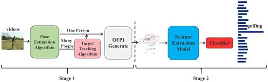
Figure 1.
The overall pipeline of our action recognition method.
The following are the main contributions of this paper:
- We propose the OFPI method for pose-based action representation;
- We extensively studied OFPI representation and CNN architectures for action classification and attempted to apply the transformer to the field of action recognition with superior performance.
Overview of our action recognition method:
Stage 1. OFPI representation
- (A)
- Joint coordinate extraction;
- (B)
- Target-person selection (multiple-person situation);
- (C)
- OFPI generation.
Stage 2. Action recognition
- (D)
- Feature extraction;
- (E)
- Action classification.
2. Related Works
The key to human action recognition based on pseudo-images lies in the pseudo-image design. To distinguish mutually occluding body parts, Schwarz et al. [23] used motion information obtained from the optical flow between subsequent intensity images. Ren et al. [24] proposed a skeleton-based optical flow-guided features method by encoding different geometric relational features into static color texture images. In particular, temporal variations in different features are converted to color variations in their corresponding images. A multi-stream CNN model is then employed to extract the discriminative patterns in the converted images for further classification. Lee et al. [25] proposed a method to extract optical flow information from the skeleton data in order to solve the problem of body-part motion changes in human action recognition. They designed and trained different KNN models and deep convolutional neural networks on the obtained images (D-CNN) and classified them. Choutas et al. [21] recently proposed PoTion, which encodes temporal information in the heat map of human joints with colors and uses this stacked colored joint heat map as the CNN model input for classifying actions. For optimal performance in method application, they combined this approach with other multi-stream methods. However, most of these techniques are too complex to meet the real-time requirements of autonomous systems. To address this issue, Dennis et al. [20] proposed a more streamlined process in which noisy human poses are encoded into an image-like data structure (EHPI) for a predetermined amount of time. The data are then fed into a simple CNN model for action recognition that encodes the skeletal data of human poses as RGB-like images and does not fully exploit the spatial and temporal characteristics of human poses. In addition, these methods employ CNN network architectures that lack a global perspective and are incapable of fully extracting pseudo-image features.
Compared with the traditional pseudo-image-based methods, the pseudo-images we designed did not simply stitch the coordinates of human joints. First, they connected the joints of the same body part in different frames in chronological order to constitute the motion trajectory of each joint point and then aggregated these joint point trajectories together according to the natural structure of the human body. The advantage of such a construction is that it makes full use of the structural features of human skeletal data, and it can intuitively observe the changes in the trend of human joint points over time.
3. OFPI Representation
In the following sections, we describe the novel pose-based action representation, OFPI. Its main steps are shown in Figure 2. In Section 3.1, we explain how to acquire human joint coordinates for each frame. In Section 3.2, we describe the steps for locating the target individual when there are multiple individuals in a single sample. In Section 3.3, we demonstrate how the acquired skeletal data are transformed into the OFPI representation.
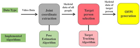
Figure 2.
The overall pipeline of OFPI representation.
3.1. Joint Coordinate Extraction
Most advanced pose estimation algorithms produce a human joint heat map or joint point coordinates along with a confidence level as output. Our representation of the OFPI was based on its joint coordinates. OpenPose is a multiple-person pose estimation algorithm that does not increase its running time with the number of people in the video and is robust enough for occlusion and truncation. The algorithm detects joints and connects them by computing part affinity fields (PAF) in order to associate various candidate joints with instances of human pose. In this work, only the joint point detection portion of the algorithm was utilized, where represents a set of two-dimensional confidence maps of predicted body-part locations. The set has confidence maps, one per part where () represents the size of the confidence map, and . In order to calculate the loss function in Equation (1) during joint point detection, more accurate joint point coordinates were regressed. An individual ground-truth confidence map for each body part of each person needed to be generated from the annotated 2D key points with Equation (2). Each confidence map was a 2D representation of the belief that a particular body part could be located in any given pixel. For a body part, when there were multiple ground-truth confidence maps, each confidence map was aggregated by the maximum operator using Equation (3). In order to ensure the accuracy of each peak, the one with the largest value was selected as the final true confidence map .
In Equation (1), represents the binary mask with when the annotation is missing at pixel , which is not counted if a key point annotation is missing. This mask is used to avoid penalizing the true positive prediction during training. In Equation (2)
indicates the real position of the person ’s body part in the picture; indicates pixel point; controls the spread of the peak.
OpenPose was operated on each video frame to obtain the joint point information for all frames in each sample. We studied the action recognition of a single person, and while there may have been multiple persons in a data sample for a single person, there was only one target person. During the application process, we discovered that OpenPose was disadvantaged when processing videos with multiple people, specifically for the JSON file generated to store the skeleton point coordinates. As the storage position of the same person in the file generally differed between frames, it was more challenging to extract the skeletal point data.
3.2. Target Person Selection
To address the aforementioned issues, we developed a pose-based target tracking algorithm capable of accurately locating the same target person in each video frame containing multiple persons. Usually, in adjacent frames, the displacement deviation and joint changes of the same character are the smallest. Therefore, the main research idea for this algorithm was to calculate the deviation between each character and the corresponding coordinates of the target character between adjacent frames. The smaller the deviation, the greater the possibility of becoming the target character. At the same time, for each joint point coordinates of the human body, we first adopted the form of the sum of the coordinates and then calculated the deviation. On the one hand, this form was more intuitive, and the calculation was simple and easy to understand. More importantly, through the actual effect of the application in the dataset we used, we could accurately locate the target person in each frame. Before performing the target tracking algorithm, we needed to determine the target person in the first frame to facilitate subsequent related calculations. Since there were few multi-person samples in the data set we selected, we could manually select the target person in the first frame and record their joint point coordinates. Following this is the general flow of the algorithm, taking the target person in frame 2 as an example.
The first step was to calculate the coordinate sum of the target person. Specifically, the sum of and coordinates of each joint point of the target person was determined using Equation (4). For 15 joint points, after calculation, there were 15 sums of coordinates .
Here, represents the th joint point (), and , represent the coordinate values of the th joint.
The second step was to calculate the coordinate sum of each person in frame 2. Specifically, the sum of the and coordinates of each joint point of each person in frame 2 was found using Equation (5). For individuals in the second frame, it was necessary to compute the sum of the coordinates of each of the people . It was necessary to compute the sum of the coordinates of each node for each individual .
Here, represents the th person in the nd frame; represents the th joint point; and , represent the coordinate values of the th joint.
The third step was to calculate the deviation between each person and the target person. Specifically, the coordinates of the target person and each person from frame 2 were differentially calculated for each human joint. The absolute values were then extracted with Equation (6) .
The fourth step was to record the number of persons corresponding to the minimum deviation of each joint. Specifically, every individual in frame 2 was assigned a number, including n numbers for n individuals. For each human joint point, the joint point with the smallest deviation was selected, and its corresponding individual number was recorded. Presuming that a human skeleton has 15 joint points, 15 numbers would be recorded.
The fifth step was to select the human body number with the most occurrences. Specifically, the recorded individual numbers were tallied. The person with the highest number of occurrences had the highest similarity to the human skeleton of the target person and was selected as the target person for the current frame. Additionally, depending on the reselected target person, the preceding steps were repeated to locate the target in each frame.
The above comprises the complete content of the pose-based human tracking algorithm we designed. The conventional method differs from our method in that it directly sums all the coordinates of each skeleton and computes the difference between them. Moreover, the individual with the smallest skeletal difference is selected as the target for the next image. Although the conventional method appears simplistic, it requires an extremely high level of completeness of the skeletal data and neglects the fact that the skeletal data obtained by the pose estimator typically contain issues such as missing joints or estimation biases. In this case, the final summation of skeletal data for two distinct individuals may be approximately the same, negatively impacting the selection of the final target individual. To overcome these limitations of the conventional method, rather than summing the coordinates of all joints in an individual as a whole, the human tracking algorithm we devised above used each human joint point as a unit to calculate the deviation between each person and the target person at each joint point. The advantage of this design is that it can eliminate the influence of other human body joint points on the currently calculated joint point deviation and reduce the impact of pose estimation error on the experimental results. Our experimental results indicated that this method could accurately localize the intended person.
3.3. OFPI Generation
Generation of OFPI representation. Because of the pose estimator error or human occlusion, it was inevitable that the skeletal point coordinates would appear at (0,0) after obtaining the target person skeletal data. On the one hand, because our OFPI representation was generated for each human joint, it was necessary to connect the same joint point in different frames in order to obtain the motion trajectory of that joint point. If (0,0) appeared in the middle, this would cause the motion trajectory of that joint point to deviate and would also obscure the motion trajectory of other joints, thereby affecting the overall OFPI representation. On the other hand, given the relatively small displacement of the same joint between two adjacent frames, even deleting a few frames would not affect the entire joint motion trajectory. Therefore, before constructing the OFPI representation, the coordinates were eliminated, thereby mitigating any negative effects on the experimental results. The final step in constructing the OFPI representation consisted of aggregating these skeletal point coordinates over time. There were two main steps in the generation of OFPI (Figure 3). For ease of understanding, we visualized the obtained skeletal data in Figure 3A. For each skeleton sequence, we focused on each skeletal point trajectory. The first step was to combine the joint points of a single component. The joints at the same position on the human body in different frames were aggregated based on the time sequence. Specifically, joint points at the same position in different frames were connected so that the trajectory of joint points changing over time could be described more accurately and intuitively (Figure 3B). We select 15 skeletal points on the human body, generating 15 motion trajectories. The second step was to aggregate the joint points of the various components. According to the natural structure of human joints, we combined the motion trajectories of 15 joints into one image. That is, the motion trajectories of the head joint points were placed at the position of the head in the human body structure, and the motion trajectories of other joint points were placed in their corresponding human body part to obtain a global understanding of the motion of each joint in the human body. Finally, the final OFPI representation was generated.
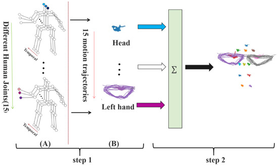
Figure 3.
Flowchart of OFPI generation. (A) Visualization of skeletal data. (B) The trajectory of joint points changing over time.
Features and advantages of OFPI representation. The OFPI representations of four different action categories are listed in Figure 4. We used different colors to represent and describe the motion of each joint in order to more intuitively distinguish the motion trajectories of different joints. Observing Figure 4, we found that the different motion categories were clearly distinguished by the OFPI encoding, which further illustrates the feasibility and effectiveness of encoding skeletal points into OFPI for motion recognition. We also discovered through observation that the motion trajectories of different joints varied. Active joints had more complex motion trajectories and a greater range of motion than inactive joints, with a limited range of motion. In addition, the motion trajectories of the active joints varied from one action to the next, resulting in a wide range of OFPI representations. This result is a significant contribution to the improvement of action recognition accuracy. When viewed as a whole, the OFPI representation illustrates the trend of various joint points over time, thereby reflecting temporal characteristics. Additionally, the shift in human posture could be observed, reflecting the spatial characteristics. Our method combined temporal and spatial characteristics of skeletal data into a single map, exploiting the kinematic characteristics and structural information of human poses. During the process of OFPI drawing, we discovered that if a few coordinate points were missing in the middle when the same coordinates in different frames were connected, it had little effect on the overall OFPI representation and action recognition accuracy. Consequently, the requirements of the pose estimation algorithm were reduced. Compared with conventional video-based action recognition, our method transformed the action information of a video sample into a single image based on the human pose trend, drastically reducing memory usage.
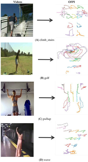
Figure 4.
Listing of OFPI representations for different action categories. (A) climb_stairs, (B) golf, (C) pullup, and (D) wave.
3.4. Example
The example shown here illustrates the principal part of OFPI representation. In order to understand the entire process of our action recognition method more intuitively and clearly, we took a clapping sample in the KTH dataset for a detailed introduction. Figure 5A shows the input video data of the clapping action. In Figure 5B, the video data were processed by the pose estimation algorithm to obtain the skeleton data of the human body, and in Figure 5C, the acquired skeleton data were encoded to generate OFPI representation. Figure 5D shows the generated OFPI representation sent to the feature extraction model for feature extraction to perform the next classification according to the extracted features using the CNN model and the transformer model. In Figure 5E, the extracted action features were sent to the classifier for action classification. Different actions usually have different features, so the classifier distinguished different action categories according to these features to finally output the correct action category.
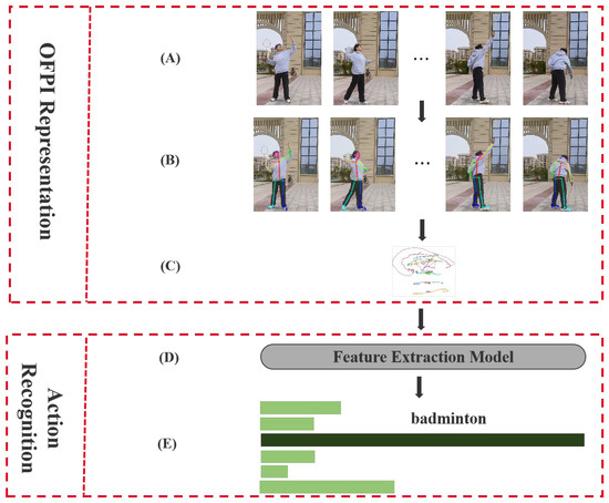
Figure 5.
An intuitive pipeline of action recognition results of the JHMDB dataset. (A) Video input; (B) skeleton extraction; (C) OFPI generation; (D) feature extraction; (E) action classification.
4. Models
This section describes the network models used to categorize OFPI representations. Section 4.1 presents the CNN-based model for action recognition. Section 4.2 introduces the transformer-based action recognition model.
4.1. CNN on OFPI Representation
4.1.1. Model Structure
Since OFPI representation has significantly less texture than standard images, the network architecture does not need to be deep and does not require any pretraining. We proposed a structure consisting of six convolutional layers and one fully connected layer. An OFPI representation with all joints stacked was the input of the network. As depicted in Figure 6, our architecture consisted of three blocks with two convolutional layers in each block for feature extraction of input data, where the kernel size of all convolutions was three and the convolution step size was one. When the spatial resolution decreased, the number of channels simultaneously doubled, beginning with 64 channels in the first block. After each convolutional layer, batch normalization and ReLU nonlinear activation were performed. After three convolutional blocks, we performed a spreading operation on the extracted feature maps and then classified actions using a fully connected layer with Softmax. In our experiments (Section 5), we examined a number of variants of this architecture with different numbers of blocks, channels, and convolutional layers. Finally, we compared our experimental results to those of PoTion to demonstrate the superiority of the OFPI.
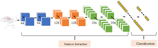
Figure 6.
CNN-based action recognition model structure.
4.1.2. Shortcomings of the CNN Model
As a consequence of its translation invariance and localization capabilities, CNN has a natural advantage in resolving image problems and has achieved success. However, one of the most significant shortcomings of CNN is the lack of global vision, which makes the CNN model unable to fully extract all features of OFPI representation, thus affecting the accuracy of action recognition. For action recognition based on pseudo-images, extracting and encoding features from multiple consecutive frames of an action video sample into pseudo-images is necessary before performing action recognition. There is typically useful information between non-adjacent frames, making the global field of view crucial. CNN’s perceptual field is constrained by the size of the convolutional kernel and the use of pseudo-images for feature extraction. It may only capture the characteristics of the two or three adjacent frames but not the relationship with more distant frames, making it impossible to fully extract the action information from the pseudo-images. Consequently, the accuracy of action recognition may be compromised. The only way to obtain a larger perceptual field with CNN models is to continuously stack convolutional layers. Nevertheless, this approach usually increases model complexity, reduces the operation rate, generates additional issues, and is not particularly accurate. The self-attention mechanism of a transformer relates to global information modeling, so its perceptual range encompasses the entire picture. In order to address the issue of CNN’s limited global field of view and to fully extract the features represented by OFPI, we sought to improve the performance of action recognition by employing the transformer model instead of the CNN module.
4.2. Transformer on OFPI Representation
4.2.1. Model Structure
The transformer model-based basic architecture consisted of three parts, shown in Figure 7A: the input-side adaptation, the feature extraction module for feature extraction, and the fully connected layer with Softmax to classify actions.
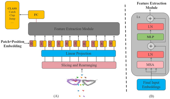
Figure 7.
Transformer-based action recognition model structure. (A) The transformer model-based basic architecture; (B) the basic structure of feature extraction module.
Input-side adaptation. The first step entailed configuring the input data. An image data illustrative of an OFPI representation of all stacked joints served as the network’s input. The feature extraction module cannot directly process the image data, and thereby, it was necessary to slice and rearrange the original two-dimensional image data into a series of two-dimensional patches , where is the number of generated patches (Equation (7)). Then, the size of each patch was converted to the size of the input vector of the feature extraction module by the vector . The feature extraction module uses constant latent vector size through all of its layers. Since the model used only the encoder module in the transformer, which had only an encoding process and no ability to integrate the encoded information into the output, the information could not be integrated into the output (i.e., decoding). A learnable vector class was added to integrate the information so that classification could be performed. The position information was lost after the image was cut and rearranged, so a learnable vector was added as the position encoding, and the position encoding vector and the patches vector were added directly to form the feature extraction module’s input (Equation (8)).
In the equation above, represents the original image’s resolution, denotes the resolution of each patch, and is the number of channels.
Feature extraction module. The input data were configured and fed into the feature extraction module to extract features. As depicted in Figure 7B, the feature extraction module was composed of layers of alternating multiheaded self-attentive mechanism (MSA) and MLP blocks, as shown in Equations (9) and (10). Layernorm (LN) was applied after each module, and the residual connection was applied after each module to improve the model’s training speed and accuracy, prevent overfitting, and make the model more robust. When MSA was implemented, self-attentive modules were applied to the input sequence (). Instead of performing a single attention function with -dimensional keys, values, and queries, we found it beneficial to linearly project the queries, keys, and values times with different, learned linear projections to , , and dimensions, respectively, where , , and are the dimensions of the queries, keys, and values vectors in each sub-header. The output of the multiheaded attention module was obtained by linear variation after the concatenation of the outputs from the various heads with Equation (11). The size was also , and multiheaded attention enabled the model to simultaneously concentrate on information from distinct representation subspaces at distinct locations. Thus, this provided multiple opportunities for focus, thereby enhancing the model’s performance.
In Equations (9)–(12), the projections of each head were parameter matrices , , , and . Because of the reduced dimension of each head, the total computational cost was similar to that of single-head attention with full dimensionality. Finally, the output of all heads was integrated through the parameter matrix to obtain the output of the final multihead self-attention mechanism.
Fully connected layer module. After extracting the features represented by OFPI through the feature extraction module, the final fully connected layer module with Softmax classified the extracted features according to the actions. Additionally, the number of output categories of the model corresponding to the input dataset was considered. For example, in the JHMDB dataset with 21 categories of actions, all 21 probability values were predicted for different actions by the fully connected layer with Softmax, and the action class with the highest probability value was determined as the final predicted action, as shown in Figure 1, stage 2.
4.2.2. Global View
The transformer model has a global perspective because of its self-attentive mechanism. The attention mechanism comprised three concepts: query, key, and value, with key and value occurring in pairs. However, for the self-attentive mechanism, query, key, and value all originated from the same input sequence . In practice, we computed the attention function on a set of queries simultaneously and packed them into the matrix , , by linear transformation as the input of the self-attention mechanism (Equation (13)). To calculate similarity, the dot product of each query and each key was calculated separately. Then, it was divided by the scaling factor to eliminate the effect of the dot product’s variance. Finally, the weight of the value was determined by applying the function Softmax. The output matrix was determined using Equation (14). According to the preceding equation, the computation was matrix-based and can be parallelized to increase operation speed. The dot product of each query with all keys was calculated separately in the self-attentive mechanism until all queries were calculated, and this enabled the transformer to perform global information modeling. Consequently, it had a global perspective and could extract OFPI-representative features more effectively.
4.2.3. Model Setting
In the application process based on the transformer model, we employed a migration learning strategy with the ViT model [26] that was pretrained on the ImageNet large dataset. First, the original model’s pretraining parameters for the feature extraction module were frozen. After that, for the subsequent classification, the MLP head module was removed and replaced with a fully connected layer corresponding to the action category of our dataset. Finally, the model was trained using the JHMDB dataset. We concentrated on tuning the hyperparameters and altering only the batch size, learning rate, and number of epochs to determine how to train the network quickly and reliably. Initial training was conducted with an initial learning rate of 0.001 and a standard momentum of 0.90 and 100 epochs, using L2 regularization with a decay weight of to offset overfitting and stochastic gradient descent (SGD) for optimization. The best experimental results were obtained for the JHMDB dataset when the learning rate was set to 0.005, and the epoch was set to 800. In the case of the JHMDB dataset, with OFPI as the input, training the transformer model on a single GPU took less than 4 h. In other words, the video classification training could be performed in a few hours on a single GPU. This result contrasts to most state-of-the-art approaches, which typically take hours or even days on multiple GPUs [4]. Taking JHMDB dataset training as an example, a chained multi-stream network [3] spent over 10 h on a single GPU to train its model and obtained model recognition accuracy of 76.1%, compared with our method, which, in addition to a much shorter training time, achieved a much higher model recognition accuracy of 93.8%. Meanwhile, PoTion [21] combined with I3D [4] achieved a training accuracy of only 85.5% on multiple GPUs, which is significantly lower than the recognition accuracy achieved by our method trained solely on a single GPU.
In this paper, the training and performance testing of all our models were carried out on a small server with NVIDIA RTX 3090 GPUs, and only a single GPU was used throughout the experiment. The construction and training of the entire model were carried out under the PYTORCH framework, using PYTORCH version 1.9.0. The PYTHON version used was 3.8 while running Ubuntu20.04 with CUDA11.2 and CUDNN8.0.5.
5. Experiment
In this section, we provide extensive experimental results for OFPI. In Section 5.1, we first introduce the dataset and setup, and Section 5.2 then examines the CNN architecture’s parameters. The superiority of OFPI is confirmed by analyzing the experimental results in Section 5.3. Finally, in Section 5.4, we compare our approach to other contemporary techniques.
5.1. Dataset and Setting
5.1.1. Dataset
JHMDB [27] is a dataset for action recognition comprising 960 video sequences corresponding to 21 actions (Figure 8), such as brushing hair, playing golf, or swinging baseball. It is a subset of the larger HMDB51 dataset comprised of digitized motion pictures and YouTube videos. It only annotates a portion of the HMDB, with 21 classes containing only one person’s actions, and removes some samples in which the person’s identity is visible. Each class contains 36–55 samples, and each sample contains 14–40 frames. See the Supplementary Material for how to obtain the dataset.
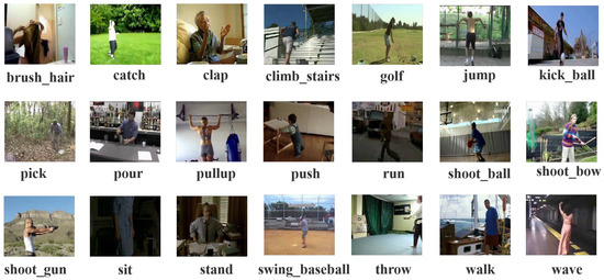
Figure 8.
JHMDB dataset with a total of 21 types of actions.
The KTH dataset encompasses six types of actions performed by 25 persons across four distinct settings, including clapping, waving, boxing, jogging, running, and walking. The video samples in this database feature changes in scale, clothing, and lighting. However, their backgrounds are relatively uniform, and the cameras are stationary. See the Supplementary Material for how to obtain the dataset. This dataset is relatively simple and was used as an experimental dataset for pseudo-image design and model training in this paper. We first employed this KTH dataset to evaluate the viability of pseudo-image design and model selection. The framework was then trained on a larger dataset to improve its efficiency.
5.1.2. Data Enhancement
For the skeletal data obtained from the pose estimation algorithm, it was necessary to reduce the influence of the pose estimation algorithm’s error on the experimental results and the impact of incorrect samples on the recognition accuracy of the OFPI representation. Therefore, we conducted an appropriate data-cleaning process to eliminate a small number of samples with completely inaccurate pose estimation while retaining the remaining samples. In addition, to address the unequal distribution of the number of samples for each action category in the JHMDB dataset, we increased the number of samples for the action category with the fewest samples. This resolution aimed to achieve a balanced number of samples, as shown in Figure 9. The treatment consisted of reusing categories with fewer samples within the same category for action categories with fewer samples. To enhance recognition, we also performed flip enhancement on the experimental data set, and the experimental results demonstrated that the flip enhancement had a positive effect.
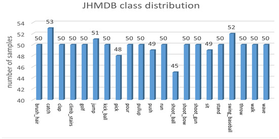
Figure 9.
Number of samples per category in the JHMDB dataset after data balancing.
5.2. CNN on OFPI
As depicted in Figure 6, we compared various CNN network architectures in which a network consisted of multiple blocks. To determine the optimal CNN network architecture, we constructed a variety of CNN network variants with varying numbers of blocks and channels in convolutional layers. The performance of various architectures is displayed in Table 1. In the JHMDB dataset, the performance of the architecture with two blocks was slightly inferior to the architecture with three blocks, as shown in Table 1. This was possibly due to the small number of convolutional layers that could not adequately extract features. Accuracy was lowest with four blocks, and the performance decreased due to overfitting. The architecture with three blocks, each with two convolutions and three blocks with 64,128,256 convolutional layers, achieved the highest accuracy of 68.9%, followed by an accuracy of 79.2% after the data were flipped and enhanced. This architecture was consequently chosen as the final CNN recognition model. To demonstrate the superiority of the OFPI representation, we compared it with the advanced pose-based action representation technique PoTion. The experimental results indicated that OFPI was generally more accurate than PoTion.

Table 1.
Comparison of the recognition accuracy with PoTion under different convolutional layer models.
5.3. Ablation Experiments
5.3.1. Comparison of OFPI Results in CNN and Transformer Models
Observing Table 2 results for the JHMDB dataset, we discovered that for both the original JHMDB dataset and the flip-enhanced dataset, the accuracy after transformer model training was typically higher than after the CNN model training. After CNN model training, the highest accuracy of OFPI was only 68.9%, which is significantly lower than the result of 78.2% obtained after the transformer model training. Moreover, there was some room for additional improvement after accuracy improvement by flipping. Furthermore, the maximum improvement was only 10%, considerably less than the transformer model’s 16%. The experimental findings indicated that the transformer-based action recognition model could extract OFPI features more effectively. Consequently, it validated the viability of the transformer for pseudo-image-based action recognition tasks. Additionally, it should be noted that the experimental results presented in the subsequent sections were all based on the transformer model training.
Table 2.
Comparison of CNN and transformer model results.
5.3.2. Effect of the Different Number of Skeletal Points on Experimental Results
Our methodology was based on the recognition of skeletal points in action. First, we investigated the impact of the number of skeletal points on the experimental outcomes, analyzed the skeletal points, and selected several representative numbers of skeletal points for the subsequent experiments (Figure 10). The comparison revealed that when the number of skeletal points n = 15, the recognition accuracy of the encoded OFPI representation was relatively high (Figure 11). Consequently, n = 15 skeletal points were selected for encoding.
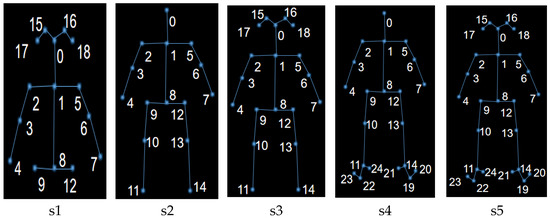
Figure 10.
Human skeleton diagram corresponding to the different number of selected skeletal points. s1: n = 15 (upper body); s2: n = 15; s3: n = 18; s4: n = 21; s5: n = 25.
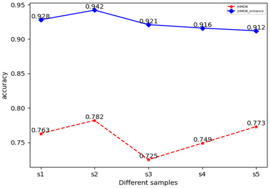
Figure 11.
Comparison of accuracy based on the JHMDB dataset with a different number of skeletal points selected. Red is the original dataset; blue is the enhanced dataset after flipping.
5.3.3. Effect of Flip Enhancement on the Accuracy of OFPI
To determine the impact of flip enhancement on experimental outcomes, we compared training performance with and without flip-data enhancement (as in Table 3). The experimental results demonstrated that this data-enhancement strategy was effective for the JHMDB dataset, resulting in a 16% increase in the accuracy of JHMDB, but had a negligible impact on the precision of the KTH dataset. We determined that the flip enhancement had little effect on the KTH dataset because it had few action categories (simple and standard) and had already learned the characteristics of different action categories well before the flip enhancement. However, the JHMDB dataset had relatively more action categories, and the videos for the same action categories came from the network. Evidently, there were distinctions between various categories. Even within the same motion category, there were differences between moving objects, and the model could not fully extract the features of each motion category using only the existing data samples. Consequently, it needed to be flipped for data expansion. In all subsequent experiments, we used flipped data augmentation for the JHMDB dataset.
Table 3.
Recognition accuracy with and without flip augmentation during training.
5.3.4. Analysis of Experimental Results
Loss value vs. accuracy line graph analysis. Observing the changes in loss values and accuracy rates on the ViT model for the JHMDB and the KTH datasets, as depicted in Figure 12, provided a clearer understanding of the model’s training. Moreover, when epochs were around 800, the loss values and accuracy rates tended to be stable for the JHMDB dataset. In addition, the line graph provided a more intuitive indication that the accuracy rate was vastly improved following the data-flip enhancement (Figure 12B). This again demonstrated the efficacy of the flip enhancement. Observing the KTH dataset before the data-flipping enhancement in Figure 12C, we found that the accuracy and loss values of the model stabilized when training at around 200 epochs, and the accuracy rate reached more than 95%, indicating that the model was well-trained. In Figure 12D, we found that after the data-flip enhancement, the accuracy and loss value of the model did not change compared with the previous one, but the model stabilized when the training epochs were around 800. We concluded that the main reason was that before the data-flip enhancement, the model could fully extract the features of each action category from the original dataset, and the extracted features were sufficient to distinguish different action categories. Thus, the accuracy rate before the data enhancement was very high. At the same time, because of the flip enhancement, this method mainly enhanced the original features in the original data set and did not provide too many new features, resulting in only a minor improvement in the accuracy rate. On the contrary, because of the increase in data samples after data-flip enhancement, the model needed more epochs to fully extract the features, which increased the training time.
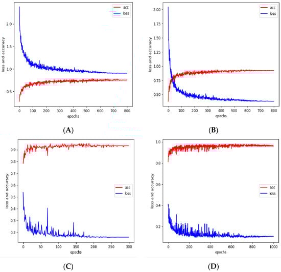
Figure 12.
Line graph of loss value vs. accuracy with epochs for JHMDB and KTH datasets: (A) JHMDB; (B) enhanced JHMDB; (C) KTH; (D) enhanced KTH.
Confusion matrix analysis. Applying the confusion matrix (Figure 13), we evaluated the performance of the model on each category of the two datasets. Simultaneously, we computed the precision, recall, and specificity of the model corresponding to each category (Table 4 and Table 5). It was observed intuitively which categories were difficult to differentiate and had lower accuracy. According to Figure 13, the three categories of jump, golf, and shooting ball had relatively high recognition accuracy in the JHMDB dataset, while recognition accuracy was lower for the categories of running and walking. In the KTH dataset, the recognition accuracy of the categories jogging and running was relatively low. We analyzed the KTH dataset experimental results by observing Figure 13C and found that the prediction results of the three categories of boxing, clapping, and waving were essentially correct. This result further illustrated that for vastly different actions, OFPI could fully reflect the characteristics unique to each action category so that the model could make predictions more easily. At the same time, observing the experimental results for walking, jogging, and running in Figure 13C, we found there were individual sample prediction errors among these three categories because the three types of action were very similar to each other. However, most samples could make correct predictions. More importantly, the misprediction of the jogging action category was only predicted as walking and running, and not as other categories with largely different motions. The same was true for samples of running and walking mispredictions, further illustrating the superiority of OFPI representation from the side, reflecting its ability to make full use of bone data. In Table 4, a comparison of various categories of indicators before and after the data-flip enhancement reveals that after the enhancement, the accuracy of the running category rose from 0.444 to 0.952, and the recall rate was enhanced from 0.400 to 1.000. The accuracy of the walking category was elevated from 0.462 to 0.870. The recall rate increased from 0.600 to 1.000, and the corresponding indicators for the other categories were also somewhat improved.
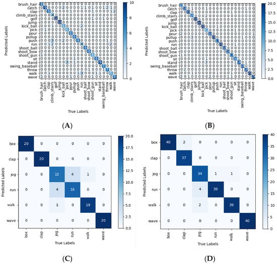
Figure 13.
Confusion matrix of JHMDB and KTH dataset: (A) JHMDB; (B) enhanced JHMDB; (C) KTH; (D) enhanced KTH.
Table 4.
Comparison of indicators before and after flipping enhancement of the JHMDB dataset.
Table 5.
Comparison of indicators before and after flipping enhancement of the KTH dataset.
5.4. Comparison with Advanced Technologies
In order to achieve 85.5% overall performance on the JHMDB dataset, traditional pseudo-image-based methods for skeleton-based action recognition typically integrate action detection with pose with multi-stream methods, such as PoTion with a multi-streaming method I3D. There are relatively few pure pose-based action recognition methods, and for certain real-time-sensitive application scenarios, such as EHPI, pure pose-based action recognition can be executed at a faster rate. Therefore, the key to pure pose-based action recognition is designing pseudo-images that utilize skeletal data more effectively. We designed a novel pseudo-image while comparing ours to other works that report the outcomes of pose-based algorithms. As shown in Table 6 below, our method achieved good results with significantly higher accuracy than pose-based action recognition technologies such as PoTion [21] and EHPI [20]. Additionally, it outperformed numerous multi-stream action recognition strategies (Table 7).
Table 6.
Average classification accuracy of the JHMDB dataset compared to other purely pose-based algorithms.
Table 7.
Average accuracy per category on the JHMDB dataset compared with state-of-the-art methods.
6. Conclusions
In this paper, we introduced the OFPI method for pose-based action representation. We first collected skeletal data using a sophisticated pose estimator. Leveraging the human tracking algorithm, we located the target person and extracted their skeletal data. The final OFPI representation was obtained by temporally aggregating these skeletal data. We attempt to apply the transformer to action recognition in order to obtain the global field of view and complete feature extraction of OFPI. The experimental results demonstrate that OFPI is capable of fully exploiting the spatiotemporal characteristics of skeletal data. Moreover, the performance of the transformer-based model is considerably superior to that of the CNN-based model. This result exemplifies the practicability of the transformer model for the pseudo-image-based action recognition task. In addition, we validated OFPI in action recognition using the KTH and JHMDB datasets. In conclusion, our approach achieves state-of-the-art performance and outperforms other pure pose-based or multi-stream-based methods.
Supplementary Materials
The following supporting information can be downloaded at the JHMDB dataset: http://jhmdb.is.tue.mpg.de/dataset, accessed on 1 January 2022; KTH dataset: https://www.csc.kth.se/cvap/actions/, accessed on 1 January 2022.
Author Contributions
Conceptualization, D.C. and T.Z.; methodology, D.C. and T.Z.; software, D.C., T.Z., C.Y., P.Z. and C.L.; validation, D.C., T.Z. and P.Z.; writing—original draft preparation, D.C., T.Z. and C.Y.; writing—review and editing, D.C., T.Z., P.Z. and C.L.; visualization, T.Z., C.Y. and P.Z.; supervision, D.C. and C.L.; project administration, D.C. and C.L. All authors have read and agreed to the published version of the manuscript.
Funding
This research was funded by Guangxi S&T Program, grant number AB17292082.
Institutional Review Board Statement
Not applicable.
Informed Consent Statement
Not applicable.
Data Availability Statement
Not applicable.
Conflicts of Interest
The authors declare no conflict of interest.
References
- Huang, Y.; Lai, S.-H.; Tai, S.-H. Human Action Recognition Based on Temporal Pose CNN and Multi-dimensional Fusion. In Proceedings of the European Conference on Computer Vision (ECCV) Workshops, Munich, Germany, 8–14 September 2018; Springer International Publishing: Cham, Switzerland, 2018; pp. 426–440. [Google Scholar]
- Tu, Z.; Xie, W.; Qin, Q.; Poppe, R.; Veltkamp, R.C.; Li, B.; Yuan, J. Multi-stream CNN: Learning representations based on human-related regions for action recognition. Pattern Recognit. 2018, 79, 32–43. [Google Scholar] [CrossRef]
- Zolfaghari, M.; Oliveira, G.L.; Sedaghat, N.; Brox, T. Chained Multi-stream Networks Exploiting Pose, Motion, and Appearance for Action Classification and Detection. In Proceedings of the IEEE International Conference on Computer Vision (ICCV), Venice, Italy, 22–29 October 2017. [Google Scholar]
- Carreira, J.; Zisserman, A. Quo Vadis, Action Recognition, A New Model and the Kinetics Dataset. In Proceedings of the 2017 IEEE Conference on Computer Vision and Pattern Recognition (CVPR), Honolulu, HI, USA, 21–26 July 2017. [Google Scholar]
- Zhang, Z. Microsoft kinect sensor and its effect. IEEE Multimed. 2012, 19, 4–10. [Google Scholar] [CrossRef]
- Cao, Z.; Simon, T.; Wei, S.E.; Sheikh, Y. Realtime Multi-Person 2D Pose Estimation Using Part Affinity Fields. In Proceedings of the 2017 IEEE Conference on Computer Vision and Pattern Recognition (CVPR), Honolulu, HI, USA, 21–26 July 2017; pp. 7291–7299. [Google Scholar]
- Fang, H.S.; Xie, S.; Tai, Y.W.; Lu, C. RMPE: Regional Multi-person Pose Estimation. In Proceedings of the 2017 IEEE International Conference on Computer Vision (ICCV), Venice, Italy, 22–29 October 2017. [Google Scholar]
- Sun, K.; Xiao, B.; Liu, D.; Wang, J. Deep High-Resolution Representation Learning for Human Pose Estimation. arXiv 2019, arXiv:1902.09212. [Google Scholar]
- Li, Y.; Xia, R.; Liu, X.; Huang, Q. Learning shape-motion representations from geometric algebra spatio-temporal model for skeleton-based action recognition. In Proceedings of the 2019 IEEE International Conference on Multimedia and Expo (ICME), Shanghai, China, 8–12 July 2019; pp. 1066–1071. [Google Scholar]
- Caetano, C.; Sena, J.; Brémond, F.; Dos Santos, J.A.; Schwartz, W.R. Skelemotion: A new representation of skeleton joint sequences based on motion information for 3d action recognition. In Proceedings of the 2019 16th IEEE International Conference on Advanced Video and Signal Based Surveillance (AVSS), Taipei, Taiwan, 18–21 September 2019; pp. 1–8. [Google Scholar]
- Caetano, C.; Brémond, F.; Schwartz, W.R. Skeleton image representation for 3d action recognition based on tree structure and reference joints. In Proceedings of the 2019 32nd SIBGRAPI Conference on Graphics, Patterns and Images (SIBGRAPI), Rio de Janeiro, Brazil, 28–30 October 2019; pp. 16–23. [Google Scholar]
- Liu, J.; Shahroudy, A.; Xu, D.; Kot, A.; Wang, G. Skeleton based action recognition using spatio-temporal LSTM network with trust gates. IEEE Trans. Pattern Anal. Mach. Intell. 2018, 40, 3007–3021. [Google Scholar] [CrossRef] [PubMed]
- Si, C.; Jing, Y.; Wang, W.; Wang, L.; Tan, T. Skeleton based action recognition with spatial reasoning and temporal stack learning. In Proceedings of the European Conference on Computer Vision (ECCV), Munich, Germany, 8–14 September 2018; Springer: Cham, Switzerland, 2018; pp. 103–118. [Google Scholar]
- Zeng, A.; Sun, X.; Yang, L.; Zhao, N.; Liu, M.; Xu, Q. Learning Skeletal Graph Neural Networks for Hard 3D Pose Estimation. In Proceedings of the 2021 IEEE/CVF International Conference on Computer Vision (ICCV), Montreal, QC, Canada, 10–17 October 2021; pp. 11436–11445. [Google Scholar]
- Yang, H.; Yan, D.; Zhang, L.; Sun, Y.; Li, D.; Maybank, S.J. Feedback Graph Convolutional Network for Skeleton-Based Action Recognition. IEEE Trans. Image Process. 2022, 31, 164–175. [Google Scholar] [CrossRef] [PubMed]
- Yan, S.; Xiong, Y.; Lin, D. Spatial Temporal Graph Convolutional Networks for Skeleton-Based Action Recognition. In Proceedings of the AAAI Conference on Artificial Intelligence, New Orleans, LA, USA, 2–7 February 2018; AAAI Press: Palo Alto, CA, USA, 2018. [Google Scholar]
- Cho, S.; Maqbool, M.; Liu, F.; Foroosh, H. Self-Attention Network for Skeleton-based Human Action Recognition. In Proceedings of the 2020 IEEE Winter Conference on Applications of Computer Vision (WACV), Snowmass, CO, USA, 1–5 March 2020. [Google Scholar]
- Yoon, Y.; Yu, J.; Jeon, M. Predictively encoded graph convolutional network for noise-robust skeleton-based action recognition. Appl. Intell. 2022, 52, 2317–2331. [Google Scholar] [CrossRef]
- Cheng, K.; Zhang, Y.; He, X.; Chen, W.; Cheng, J.; Lu, H. Skeleton-Based Action Recognition with Shift Graph Convolutional Network. In Proceedings of the 2020 IEEE/CVF Conference on Computer Vision and Pattern Recognition (CVPR), Seattle, WA, USA, 13–19 June 2020. [Google Scholar]
- Ludl, D.; Gulde, T.; Curio, C. Simple yet efficient real-time pose-based action recognition. In Proceedings of the 2019 IEEE Intelligent Transportation Systems Conference (ITSC), Auckland, New Zealand, 27–30 October 2019; pp. 581–588. [Google Scholar] [CrossRef]
- Choutas, V.; Weinzaepfel, P.; Revaud, J.; Schmid, C. PoTion: Pose MoTion Representation for Action Recognition. In Proceedings of the 2018 IEEE/CVF Conference on Computer Vision and Pattern Recognition (CVPR), Salt Lake City, UT, USA, 18–23 June 2018. [Google Scholar]
- Vaswani, A.; Shazeer, N.; Parmar, N.; Uszkoreit, J.; Jones, L.; Gomez, A.N.; Kaiser, L.; Polosukhin, I. Attention Is All You Need. arXiv 2017, arXiv:1706.03762. [Google Scholar]
- Schwarz, L.A.; Mkhitaryan, A.; Mateus, D.; Navab, N. Human skeleton tracking from depth data using geodesic distances and optical flow. Image Vis. Comput. 2012, 30, 217–226. [Google Scholar] [CrossRef]
- Ren, J.; Reyes, N.H.; Barczak AL, C.; Scogings, C.; Liu, M. An investigation of skeleton-based optical flow-guided features for 3D action recognition using a multi-stream CNN model. In Proceedings of the 2018 IEEE 3rd International Conference on Image, Vision and Computing (ICIVC), Chongqing, China, 27–29 June 2018; pp. 199–203. [Google Scholar]
- Lee, Y.T.; Pengying, T.; Yayilgan, S.Y.; Elezaj, O. Data-Driven Machine Learning Approach for Human Action Recognition Using Skeleton and Optical Flow. In Proceedings of the International Conference on Intelligent Technologies and Applications, Grimstad, Norway, 11–13 October 2021; Springer: Cham, Switzerland, 2021; pp. 163–175. [Google Scholar]
- Dosovitskiy, A.; Beyer, L.; Kolesnikov, A.; Weissenborn, D.; Zhai, X.; Unterthiner, T.; Dehghani, M.; Minderer, M.; Heigold, G.; Gelly, S.; et al. An Image is Worth 16x16 Words: Transformers for Image Recognition at Scale. arXiv 2020, arXiv:2010.11929. [Google Scholar]
- Jhuang, H.; Gall, J.; Zuffi, S.; Schmid, C.; Black, M.J. Towards understanding action recognition. In Proceedings of the IEEE International Conference on Computer Vision, Sydney, NSW, Australia, 1–8 December 2013. [Google Scholar]
- Yang, F.; Wu, Y.; Sakti, S.; Nakamura, S. Make Skeleton-based Action Recognition Model Smaller, Faster and Better. In Proceedings of the ACM Multimedia Asia, Beijing, China, 15–18 December 2019; Association for Computing Machinery: New York, NY, USA, 2019; pp. 1–6. [Google Scholar] [CrossRef]
- Du, W.; Wang, Y.; Yu, Q. RPAN: An End-to-End Recurrent Pose-Attention Network for Action Recognition in Videos. In Proceedings of the 2017 IEEE International Conference on Computer Vision (ICCV), Venice, Italy, 22–29 October 2017. [Google Scholar]
- Peng, X.; Schmid, C. Multi-region two-stream R-CNN for action detection. In Proceedings of the ECCV 2016-European Conference on Computer Vision, Amsterdam, The Netherlands, 8–16 October 2016; p. hal-01349107v1. [Google Scholar]
- Yan, A.; Wang, Y.; Li, Z.; Qiao, Y. PA3D: Pose-Action 3D Machine for Video Recognition. In Proceedings of the 2019 IEEE/CVF Conference on Computer Vision and Pattern Recognition (CVPR), Long Beach, CA, USA, 15–20 June 2019. [Google Scholar]
- Mcnally, W.; Wong, A.; Mcphee, J. STAR-Net: Action Recognition using Spatio-Temporal Activation Reprojection. In Proceedings of the 2019 16th Conference on Computer and Robot Vision (CRV), Kingston, QC, Canada, 29–31 May 2019. [Google Scholar]
- Gkioxari, G.; Malik, J. Finding Action Tubes. arXiv 2014, arXiv:1411.6031. [Google Scholar]
Disclaimer/Publisher’s Note: The statements, opinions and data contained in all publications are solely those of the individual author(s) and contributor(s) and not of MDPI and/or the editor(s). MDPI and/or the editor(s) disclaim responsibility for any injury to people or property resulting from any ideas, methods, instructions or products referred to in the content. |
© 2023 by the authors. Licensee MDPI, Basel, Switzerland. This article is an open access article distributed under the terms and conditions of the Creative Commons Attribution (CC BY) license (https://creativecommons.org/licenses/by/4.0/).