Article

Dynamic Modeling for Metro Passenger Flows on Congested Transfer Routes

1
School of Science, Beijing University of Civil Engineering and Architecture, Beijing 100044, China
2
School of Mathematics, Physics, and Statistics, Shanghai University of Engineering Science, Shanghai 201620, China
3
NCMIS, KLSC, Academy of Mathematics and Systems Science, Chinese Academy of Sciences, Beijing 100190, China
*
Author to whom correspondence should be addressed.
Mathematics 2023, 11(6), 1427; https://doi.org/10.3390/math11061427
Submission received: 14 February 2023 / Revised: 7 March 2023 / Accepted: 9 March 2023 / Published: 15 March 2023
(This article belongs to the Special Issue Advances in Statistical Modeling)

Abstract

:
With the rapid development of urbanization, the metro becomes more and more important for people’s travel in big cities. To quantitatively describe metro passenger flows on congested transfer routes, this paper introduces a dynamic model based on automated data from the automatic fare collection (AFC) and automatic vehicle location (AVL) systems. An expectation maximization (EM) algorithm is proposed to compute the maximum likelihood estimates of unknown parameters in our model. Our model can yield a systematic analysis of one-transfer passenger flows on both population and individual aspects. Important characteristics, including transfer time, boarding probabilities, walking time, passenger-to-train assignment probabilities, and total travel time, can be inferred using only the AFC and AVL data. We provide a case study on the Beijing metro. Detailed analysis results based on our model are given. We also present a cross-validation method to validate our model with real data.

1. Introduction

The metro is an important component of the urban transit system. With the advantages of fast speed, punctual operation, and large load, it has become the first choice for most commuters in many big cities. There are over ten million people traveling by metro in Beijing every day [1]. In the meantime, with the rapid development of urbanization, limited numbers of metro lines and trains can no longer meet people’s travel needs. Congestion on platforms and in carriages often occurs, especially in the morning and evening peak periods. To alleviate the problem of congestion, metro administrations should develop reasonable management measures based on effective evaluation of passenger flows. Therefore, it is necessary to study and quantify characteristics of passenger flows, especially during peak hours.
The automatic fare collection (AFC) and automatic vehicle location (AVL) systems in the metro provide a great convenience for collecting data to study passenger flows. We can obtain a passenger’s OD (origin-destination) station, tap-in time, and tap-out time from the AFC data. The route and schedule of each train can be obtained from the AVL data. With the help of AFC data, [2] proposed an estimation model based on a Bayesian inference formulation to enable the study of the main stages affecting passenger travel time, i.e., walking, waiting, transfer, and in-vehicle times. Ref. [3] used AFC and AVL data to propose a comprehensive approach to estimate passenger congestion costs in terms of equivalent travel time loss. Other studies on metro passenger flows based on automated AFC and AVL data can be found in [4,5,6,7,8], among others.
Several authors studied passenger-to-train assignment models and related inferential issues concerning passenger flows on no-transfer metro routes based on automated data [9,10,11]. This paper focuses on congested transfer routes that are more challenging than no-transfer cases. There are limited papers on analysis of metro transfer routes in the literature. Refs. [12,13] developed optimization models for minimizing the transfer waiting time through modifying train schedules. They did not provide methods to infer passenger flows based on automated data. Ref. [14] proposed an equilibrium model based on train operating diagrams and used it to estimate spatial and temporal distributions of the passenger flows at transfer stations. However, this paper did not estimate specific characteristics of passenger flows such as the boarding probability, transfer time, and walking time. Ref. [15] proposed a complete method to estimate the distributions of walking time and waiting time of transfer passengers based on automated data. However, their method is valid only during off-peak periods. Actually, the issue of estimating those distributions becomes much more complicated during peak hours because of the left behind phenomenon. Ref. [16] proposed a data-driven passenger itinerary inference model to infer left behind, route choice, and probabilities of boarding feasible trains. Their model requires a certain assumption on transfer time that is difficult to verify with automated data. Some important characteristics including walking time and total travel time are not provided in [16]. Ref. [11] presented a new passenger-to-train assignment model, and extended it to one-transfer routes. However, they did not provide feasible methods to estimate the input parameters of such a model for transfer cases. Furthermore, Ref. [11] method is based on the data of the same tap-in time, which cannot be straightforwardly applied to dynamic passenger flows.
In this paper we propose a dynamic modeling method for passenger flows on congested transfer routes based on automated data. Our model constructs a probabilistic quantification relationship between a passenger’s tap-in and tap-out times. An expectation maximization (EM) algorithm [17] is proposed to compute the maximum likelihood estimates (MLEs) of unknown parameters in our model. Our model can yield a systematic analysis of one-transfer passenger flows on both population and individual aspects. In particular, inference and uncertainty quantification of transfer time, an important feature on transfer routes, are presented via our model. Other characteristics on a specific one-transfer route including boarding probabilities, walking time, passenger-to-train assignment probabilities, and total travel time can also be inferred. Our method requires only AFC and AVL data on the route under minimal assumptions. We provide a case study on the Beijing metro. Detailed analysis results based on our model are given. Our method can be validated based on real data via cross-validation.
The major contributions of this paper can be summarized as follows.
(i). We provide reasonable statistical modeling and inferential techniques for passenger flows on metro transfer routes, which constitute a comprehensive analysis on passenger flow characteristics, at both the aggregate and individual levels.
(ii). The proposed methods are completely data-driven, with only automated data. We present quantification indices as much as possible by making full use of automated data.
(iii). Based on rigorous mathematical and statistical derivation, we provide a general idea to analyze metro passenger flows. This idea can be extended to other situations.
The rest of this paper is organized as follows. Section 2 provides a literature review. Section 3 introduces the dynamic model for one-transfer routes and provides parameter estimation methods based on AFC and AVL data. Section 4 discusses applications of the proposed model to inferences for passenger flow characteristics. Section 5 provides the case study and validation of our model. Section 6 ends this paper with some conclusions.

2. Research Background

In the literature, research on metro systems is focused on two aspects: the train operation level and the passenger travel level. At the train operation level, the time interval between train departures is an important factor to describe the efficiency of passengers’ travel. A well-organized metro system often requires a reasonable train schedule. Therefore, how to alleviate the metro congestion by adjusting the train schedule has become a hot topic. Ref. [18] proposed a train timetable rescheduling method based on deep learning. This method enables real-time rescheduling of train schedules after random disturbances. Ref. [19] propose a mixed-integer optimization method to generate well-synchronized timetables, thereby reducing the transfer waiting time for transfer passengers. In fact, there are many uncontrollable random factors in metro systems. Optimization of metro system parameters should be based on accurate estimation of the uncertainty caused by these factors, which requires reasonable statistical models. However, such models have not been well developed in the literature, especially for the transfer routes.
At the level of passenger travel, quantitative indices of passenger travel behavior reflect the current situation in the metro system. Statistical or machine learning methods are used to estimate such indices. Ref. [20] developed an ensemble deep learning approach to forecast the dynamic metro passenger flow. This approach was designed for the entire metro network, and cannot accurately estimate the passenger flow indices on a certain route. Ref. [5] analyzed distributional characteristics of the travel time with AFC data, and proposed a method for estimating path-selecting proportions. Ref. [21] provided a passenger-to-train assignment method, and estimated the walking time and waiting time of metro passengers. Although the two papers analyzed the distributional characteristics of the travel time, the impact of passengers’ tap-in times was ignored in their studies. In fact, passengers who enter the station at different tap-in times face different congestion conditions. Hence, to estimate real-time characteristics of the metro system, we need the study on dynamic models for passenger flows.
Transfer is often an indispensable part of long-distance metro travel. However, the problem of estimating dynamic metrics on congested transfer routes has not received a lot of attention in the literature. This paper aims to fill such a gap, and completely data-driven approaches are proposed in the following sections.

3. Dynamic Models for Transfer Routes

3.1. Likelihood Model of Tap-Out Times

We consider a one-transfer trip in metro systems, which consists of two segments. Let segment 1 and segment 2 denote the segments from the origin to the transfer and from the transfer to the destination, respectively. The time between the tap-in and tap-out of a passenger can be divided into the following five periods:
(i).
Boarding time: the time from entering the tap-in fare gate to boarding a train on segment 1;
(ii).
Travel time on the train of segment 1;
(iii).
Transfer time: the time from getting off the train on segment 1 to boarding the train on segment 2;
(iv).
Travel time on the train of segment 2;
(v).
Egress time: the time to walk to the exit fare gate after alighting from the train of segment 2.
The flow chart of such a trip is shown in Figure 1.
For a passenger on the transfer route, denoted by Route A in the following, there may be more than one possible itinerary due to crowded platforms and carriages, especially during peak hours, and it is not determined which train he/she could take with only his/her tap-in and tap-out times. Similar to [11], we need to infer the passenger-to-train assignment and other quantification indices of passenger flows on Route A using the corresponding AVL and AFC data. We then present the following notation and definitions.
Suppose there are n passengers on Route A. Let T A i n = t A 1 i n , t A 2 i n , , t A n i n T and T A o u t = t A 1 o u t , t A 2 o u t , , t A n o u t T denote the sets of their tap-in and tap-out times, respectively. The egress times of the passengers are independently and identically distributed from the log-normal distribution L N μ A , σ A 2 with probability density function
f x | μ A , σ A = exp { ln x μ A 2 / 2 σ A 2 } / 2 π σ A 2 x 2 1 / 2 , x > 0 ,
where < μ A < and 0 < σ A < . This log-normal assumption is widely used and has been verified in the literature (e.g., [15]). Actually, our method in this paper can also be applied to the cases of other egress time distributions such as in [11].
Considering the periodicity of the train schedule, we define a train departure interval as a unit time interval 0 , 1 , which implies that the departure times of trains at the origin station are 1 , 2 , 3 , . We first handle the passengers whose tap-in times lie in 0 , 1 , i.e., t A i i n 0 , 1 , i = 1 , , n . General cases for peak hours will be discussed in Section 3.4. Mark the first train passengers can take after arriving at the origin station as Train 1 of segment 1. If a passenger takes Train 1 on segment 1, then the first train he/she can take on segment 2 is recorded as Train 1 on segment 2. Define:
D T j ( 1 ) : departure time of Train j from the origin station on segment 1 , A T j ( 1 ) : arrival time of Train j at the transfer station on segment 1 , D T k ( 2 ) : departure time of Train k from the transfer station on segment 2 , A T k ( 2 ) : arrival time of Train k at the terminal station on segment 2 , m i : the number of feasible itineraries for the passenger i of Route A , then m i = # S i , where S i = { ( j , k ) : t A i i n D T j ( 1 ) , A T j ( 1 ) D T k ( 2 ) , A T k ( 2 ) t A i o u t } = { ( j , k ) : A T j ( 1 ) D T k ( 2 ) , A T k ( 2 ) t A i o u t } , K i : the number of feasible itineraries for the passenger i of Route A on segment 2 , i . e . , K i = # k : there exists j s . t . ( j , k ) S i , and let K = max 1 i n K i , m i ( k ) : the number of feasible itineraries for the passenger i of Route A on segment 1 who takes Train k on segment 2 , i . e . , m i ( k ) = # j : ( j , k ) S i , k = 1 , , K i , where # A denotes the number of elements in the set A , and let m ( k ) = max 1 i n m i ( k ) , J = max 1 k K m ( k ) .
We have m i = k = 1 K i m i ( k ) and 1 m i ( 1 ) m i ( K i ) . For example, if S i = { ( 1 , 1 ) , ( 1 , 2 ) , ( 1 , 3 ) , ( 2 , 2 ) , ( 2 , 3 ) , ( 3 , 3 ) } , we have m i = 6 , K i = 3 , m i ( 1 ) = 1 , m i ( 2 ) = 2 , and m i ( 3 ) = 3 .
Let ρ j k ( t i i n ) denote the probability that a passenger whose tap-in time is t i i n takes Train j on segment 1 and Train k on segment 2 for j = 1 , , J , k = 1 , , K . If the passenger takes Train k on segment 2 and J > m i ( k ) , then we let ρ j k ( t i i n ) = 0 , j = m i ( k ) + 1 , , J , k = 1 , , K i . Moreover, if K > K i , then we let ρ j k ( t i i n ) = 0 , j = 1 , , J , k = K i + 1 , , K . Therefore, for each passenger on Route A entering the station at time t i n ( 0 , 1 ] , he/she has at most J K feasible itineraries, and the corresponding probabilities are ρ 11 ( t i n ) , , ρ 1 K ( t i n ) , , ρ J 1 ( t i n ) , , ρ J K ( t i n ) .
Let
η j ( t i n ) = k = 1 K ρ j k ( t i n ) , j = 1 , , J ,
denote the probability that a passenger whose tap-in time is t i n takes Train j on segment 1. Let
γ k ( t i n ) = j = 1 J ρ j k ( t i n ) , k = 1 , , K ,
denote the probability that a passenger whose tap-in time is t i n takes Train k on segment 2. Furthermore, let ρ k | j ( t i n ) denote the conditional probability that a passenger whose tap-in time is t i n takes Train k on segment 2 conditionally on the event that he/she takes Train j on segment 1, and let ρ ˜ j | k ( t i n ) denote the conditional probability that a passenger whose tap-in time is t i n takes Train j on segment 1 conditionally on the event that he/she takes Train k on segment 2. By the conditional probability formula, we have
ρ k | j t i n = ρ j k t i n k = 1 K ρ j k t i n = ρ j k t i n η j t i n , j = 1 , , J , k = 1 , , K ,
ρ ˜ j | k t i n = ρ j k t i n j = 1 J ρ j k t i n = ρ j k t i n γ k t i n , j = 1 , , J , k = 1 , , K .
Let E i k denote the event that passenger i takes Train k on segment 2. Given the tap-in time of passenger i, the distribution function of t A i o u t can be written as
P t A i o u t t = k = 1 K P E i k P t A i o u t t | E i k = k = 1 K j = 1 J ρ j k t A i i n P t A i o u t t | E i k = k = 1 K j = 1 J ρ j k t A i i n P t A i o u t A T k ( 2 ) t A T k ( 2 ) | E i k = k = 1 K j = 1 J ρ j k t A i i n F A t A i o u t A T k ( 2 ) ,
where F A is the cumulative distribution of L N μ A , σ A 2 . Taking the derivative of the above equation with respect to t A i o u t , we have the tap-out time t A i o u t which follows a mixture probability distribution with density
p A t A i o u t = j = 1 J k = 1 K ρ j k t A i i n f t A i o u t A T k ( 2 ) | θ A ,
where θ A = μ A , σ A T and f is defined in (1). According to (6), the joint density of T A o u t = t A 1 o u t , t A 2 o u t , , t A n o u t T can be given. Here, we write it as the following likelihood form,
L A φ A T A o u t = i = 1 n j = 1 J k = 1 K ρ j k t A i i n f t A i o u t A T k ( 2 ) | θ A = i = 1 n k = 1 K f t A i o u t A T k ( 2 ) | θ A j = 1 J ρ j k t A i i n ,
where φ A = θ A T , ρ T T , θ A = μ A , σ A T , and ρ ( · ) = ρ 11 · , , ρ J K · T .
It can be seen from (7) that, by maximizing it over the parameter space, we can only obtain the estimators of j = 1 J ρ j k t , k = 1 , , K , i.e., the probabilities of taking the trains on segment 2, while the value of each ρ j k t , j = 1 , , J , k = 1 , , K is inestimable. For example, assuming J = K = 2 , we have ρ t = ρ 11 t , ρ 12 t , ρ 21 t , ρ 22 t T . By maximizing (7), we can obtain estimators of ρ 11 t + ρ 21 t and ρ 12 t + ρ 22 t , and cannot estimate ρ 11 t , ρ 12 t , ρ 21 t , ρ 22 t . To overcome such an identifiability issue, we introduce a method based on auxiliary data, and discuss it in the next subsection.

3.2. Likelihood Model Combined with Auxiliary Data

Let Route B represent the route from the origin to the transfer. Passengers on Route A share segment 1 with those on Route B. Therefore, it can be assumed that they have the same boarding probabilities on segment 1. In this subsection, we introduce the AFC data on Route B as auxiliary data that help to estimate each component of ρ in (7).
Let T B i n = t B 1 i n , t B 2 i n , , t B n 0 i n T and T B o u t = t B 1 o u t , t B 2 o u t , , t B n 0 o u t T denote the vectors of passengers’ tap-in and tap-out times on Route B, respectively. Like in Section 3.1, we assume t B i i n ( 0 , 1 ] for i = 1 , , n 0 . Assume further that the distribution of egress time on Route B is L N ( μ B , σ B 2 ) . Given t B i i n , the tap-out time t B i o u t follows the following mixture probability distribution with density
p B t B i o u t = j = 1 J f t B i o u t A T j ( 1 ) | θ B k = 1 K ρ j k t B i i n ,
where θ B = μ B , σ B T , and f is defined in (1). The likelihood function based on T o u t = T A o u t T , T B o u t T is
L φ T o u t = i = 1 n k = 1 K f t A i o u t A T k ( 2 ) | θ A j = 1 J ρ j k t A i i n · i = 1 n 0 j = 1 J f t B i o u t A T j ( 1 ) | θ B k = 1 K ρ j k t B i i n ,
where φ = θ A T , θ B T , ρ T . Maximum likelihood estimators (MLEs) of unknown parameters φ , including each ρ j k t , j = 1 , , J , k = 1 , , K , can be computed by maximizing (8). The use of T B i n and T B o u t overcomes the identifiability issue with only the data on Route A.
Note that ρ ( · ) are unknowns functions, and that it is hard to find their MLEs. We use the quadratic logistic function to parameterize them, and assume
ρ j k t | β = exp β j k t ˜ 1 + j = 1 J 1 k = 1 K exp β j k t ˜ + k = 1 K 1 exp β J k t ˜ , j = 1 , , J , k = 1 , , K , ( j , k ) ( J , K ) , ρ J K t | β = 1 1 + j = 1 J 1 k = 1 K exp β j k t ˜ + k = 1 K 1 exp β J k t ˜ ,
where t ˜ = 1 , t , t 2 T , β = β 11 T , , β J ( K 1 ) T T , and β j k = β 0 , j k , β 1 , j k , β 2 , j k T for j = 1 , , J , k = 1 , , K , ( j , k ) ( J , K ) . Plugging (9) into (8), we have
L φ t T o u t = i = 1 n k = 1 K f t A i o u t A T k ( 2 ) | θ A j = 1 J ρ j k t A i i n | β · i = 1 n 0 j = 1 J f t B i o u t A T j ( 1 ) | θ B k = 1 K ρ j k t B i i n | β ,
where φ t = θ A T , θ B T , β T T is a ( 3 J K + 1 ) -dimensional vector of unknown parameters.

3.3. The EM Algorithm

This section proposes the EM algorithm [17] to compute MLEs of φ t in (10). We first introduce two types of hidden variables as follows.
U i , k : the indicator of the event that passenger i on Route A took Train k on segment 2 , i . e . , U i , k = 1 if this passenger took Train k on segment 2 ; U i , k = 0 otherwise , V i , j : the indicator of the event that passenger i on Route B took Train j , i . e . , V i , j = 1 if this passenger took Train j ; V i , j = 0 otherwise .
According to (10), the complete likelihood function can be written as
L c φ t T o u t , U , V = i = 1 n k = 1 K f t A i o u t A T k ( 2 ) | θ A j = 1 J ρ j k t A i i n | β U i , k · i = 1 n 0 j = 1 J f t B i o u t A T j ( 1 ) | θ B k = 1 K ρ j k t B i i n | β V i , j ,
where U = { U i , k } i = 1 , , n , k = 1 , , K and V = { V i , j } i = 1 , , n 0 , j = 1 , , J . The corresponding complete log-likelihood function is
l c φ t T o u t , U , V = i = 1 n k = 1 K U i , k log f t A i o u t A T k ( 2 ) | θ A + log j = 1 J ρ j k t A i i n | β + i = 1 n 0 j = 1 J V i , j log f t B i o u t A T j ( 1 ) | θ B + log k = 1 K ρ j k t B i i n | β .
The steps of the EM algorithm are as follows.
(I) Given the initial values φ t ( 0 ) = θ A ( 0 ) T , θ B ( 0 ) T , β ( 0 ) T T of the parameters.
(II) Expectation step: after the qth iteration, compute the expectation for the hidden variables U i , k and V i , j in the log-likelihood function, we have
Q φ t | φ t ( q ) = E l c φ t | T o u t | T o u t , φ t ( q ) = l 1 θ A + l 2 θ B + l 3 β ,
where
l 1 θ A = i = 1 n k = 1 K C i k ( q ) log f t A i o u t A T k ( 2 ) | θ A , l 2 θ B = i = 1 n 0 j = 1 J D i j ( q ) log f t B i o u t A T j ( 1 ) | θ B , l 3 β = i = 1 n k = 1 K C i k ( q ) log j = 1 J ρ j k t A i i n | β + i = 1 n 0 j = 1 J D i j ( q ) log k = 1 K ρ j k t B i i n | β ,
and
C i k ( q ) = E U i , k | φ t ( q ) = f t A i o u t A T k ( 2 ) | θ A ( q ) j = 1 J ρ j k t A i i n | β ( q ) k = 1 K f t A i o u t A T k ( 2 ) | θ A ( q ) j = 1 J ρ j k t A i i n | β ( q ) , D i k ( q ) = E V i , j | φ t ( q ) = f t B i o u t A T j ( 1 ) | θ B ( q ) k = 1 K ρ j k t B i i n | β ( q ) j = 1 J f t B i o u t A T j ( 1 ) | θ B ( q ) k = 1 K ρ j k t B i i n | β ( q ) .
(III) Maximization step: maximizing Q φ t | φ t ( q ) yields the ( q + 1 ) th iteration of parameter φ t , where θ A ( q + 1 ) = arg max l 1 θ A , θ B ( q + 1 ) = arg max l 2 θ B , and β ( q + 1 ) = arg max l 3 β .
(IV) Iteration: repeat steps (II) and (III) until convergence.
It can be seen that the EM algorithm simplified the original optimization problem through introducing hidden variables. Note that its performance relies on the choice of the initial values. Multiple initial values can be used to better approximate the global solution. Our experience based on numerical simulations shows that the proposed EM algorithm is efficient to compute the MLEs.

3.4. Periodic Modeling

In this paper, we focus on modeling for the transfer routes during peak hours. With train departure intervals of equal lengths, the passenger flow has stable performance. Therefore, the distribution f of egress times remains, and the boarding probabilities ρ ( t ) behave periodically. Specifically, consider train intervals ( D T j ( 1 ) , D T j + 1 ( 1 ) ] , , ( D T j + l 1 ( 1 ) , D T j + l ( 1 ) ] in such a period. The functions ρ ( t ) in any two of these intervals are identical. We construct a periodic model for ρ ( t ) to analyze the AFC data of passengers who enter the metro system during peak hours.
Without loss of generality, let j = 1 , D T k ( 1 ) = k 1 for k = 1 , , l + 1 . For t ( D T 1 ( 1 ) , D T l + 1 ( 1 ) ] = ( 0 , l ] , assume that
ρ j k t | β = exp β j k { t ˙ } 1 + j = 1 J 1 k = 1 K exp β j k { t ˙ } + k = 1 K 1 exp β J k { t ˙ } , j = 1 , , J , k = 1 , , K , ( j , k ) ( J , K ) , ρ J K t | β = 1 1 + j = 1 J 1 k = 1 K exp β j k { t ˙ } + k = 1 K 1 exp β J k { t ˙ } ,
where { t ˙ } = 1 , t ˙ , t ˙ 2 T and t ˙ = t t if t t > 0 , t ˙ = 1 otherwise. · denotes the floor function. β = β 11 T , , β J ( K 1 ) T T , and β j k = β 0 , j k , β 1 , j k , β 2 , j k T for j = 1 , , J , k = 1 , , K , ( j , k ) ( J , K ) are unknown parameters.
Clearly, (9) is a special case of (11) with l = 1 . Replacing (9) with (11) in (10), we obtain the periodicity model of ( T A i n , T A o u t , T B i n , T B o u t ) , where t A i i n 0 , l , i = 1 , , n and t B i i n 0 , l , i = 1 , , n 0 . The method to estimate the unknown parameters for l = 1 in previous subsections can also be used here.
Figure 2 is a process flow chart of the proposed methodology. The first part presents the model and the method for estimating an unknown parameter in the model. The second part provides applications of the model and estimated parameters, which will be discussed in the next section.

4. Applications of Analysis of Transfer Routes

In this section, we present some applications of our dynamic model in the previous sections for the analysis of transfer routes during peak hours. First of all, we should point out that the parameters in (8) can be viewed as measures that describe some aspects of characteristics of transfer passenger flows. Therefore, our estimators can directly be used to infer these measures. Furthermore, our method can be used to infer the transfer time and to predict the travel time on the transfer route.

4.1. Inference for the Transfer Time

Recall that a passenger’s transfer time is the time from getting off the train on segment 1 to boarding the train on segment 2. It contains transfer walking time and waiting time at the platform of the transfer station, and thus is an important index to quantify the congestion condition of the transfer channel and segment 2. Based on AFC and AVL data, this subsection studies inferences for transfer times via the proposed dynamic model.
First, we consider the population aspect, i.e., inference for the transfer time when only the tap-in time is given. By definition, the transfer time T t r a n s f e r of a passenger takes its value on a finite set { D T k ( 2 ) A T j ( 1 ) , j = 1 , , J , k = 1 , , K } . Given the passenger’s tap-in time t A i n , it is not hard to derive the distribution of the transfer time
P T t r a n s f e r = D T k ( 2 ) A T j ( 1 ) | t A i n = ρ j k ( t A i n ) j = 1 , , J , k = 1 , , K .
Therefore, the conditional mean and conditional standard deviation of T t r a n s f e r are given by
E T t r a n s f e r | t A i n = j = 1 J k = 1 K ρ j k ( t A i n ) D T k ( 2 ) A T j ( 1 ) ,
s d T t r a n s f e r | t A i n = j = 1 J k = 1 K ρ j k ( t A i n ) D T k ( 2 ) A T j ( 1 ) 2 E T t r a n s f e r | t A i n 2 1 / 2 .
The MLEs of ρ j k ( t A i n ) obtained in Section 3 can be used to compute these quantities.
Next, we consider the individual aspect, i.e., inference for the transfer time when the tap-in and tap-out times are given. To study this problem, we need the modified passenger-to-train assignment model [11],
p i j k = P passenger i takes Train j on segment 1 and Train k on segment 2 | t A i i n , t A i o u t = f t A i o u t A T k ( 2 ) ρ j k ( t A i i n ) j = 1 J k = 1 K f t A i o u t A T k ( 2 ) ρ j k ( t A i i n ) .
Consequently, the conditional probability distribution, conditional mean, and conditional standard deviation of T t r a n s f e r are given by
P i T t r a n s f e r = D T k ( 2 ) A T j ( 1 ) | t A i i n , t A i o u t = p i j k j = 1 , , J , k = 1 , , K , E i T t r a n s f e r | t A i i n , t A i o u t = j = 1 J k = 1 K p i j k D T k ( 2 ) A T j ( 1 ) , s d i T t r a n s f e r | t A i i n , t A i o u t = j = 1 J k = 1 K p i j k D T k ( 2 ) A T j ( 1 ) 2 E i T t r a n s f e r | t A i i n , t A i o u t 2 1 / 2 .
These quantities can be calculated by (14) and the MLEs of f and ρ j k . The passenger-to-train assignment model and individual inference for T t r a n s f e r can be used to infer the movement of a specified passenger in the metro system according to his/her tap-in and tap-out times.

4.2. Prediction and Validation

This subsection discusses how to predict the tap-out time of a transfer passenger when his/her tap-in time is given. Hence, the total travel time can be predicted given one’s tap-in time. The prediction method can also be used to validate our method via cross-validation (CV).
By (6), given t A i n , the conditional density function of the tap-out time t A o u t of the passenger is
p A t A o u t = j = 1 J k = 1 K ρ j k t A i n f t A o u t A T k ( 2 ) | θ A .
When the parameters are known, the predictor of t A o u t that minimizes the mean squared prediction error is the following conditional mean:
E ( t A o u t | t A i n ) = j = 1 J k = 1 K ρ j k t A i n t f t A T k ( 2 ) | θ A d t .
Plugging the MLEs of the parameters into (17), we get the empirical version of the best predictor. With the MLEs, the conditional distribution of t A o u t can be estimated via (16), and this can yield prediction intervals of t A o u t . Specifically, given a confidence level α ( 0 , 1 ) , the 100 1 α % prediction interval of the tap-out time of a passenger with the tap-in time t A i n can be given by
[ c α / 2 , c 1 α / 2 ] ,
where c α represents the lower α -quantile of the estimator of the distribution (16).
In addition, the accuracy of the above prediction method on a test sample can be used to validate the proposed model. When there does not exist a test sample, the CV method [22] can be applied. We randomly divide the current AFC data of Route A into two parts. One is used as the training sample to train the model parameters by the method in Section 3, and the other part acts as the test sample that is used to evaluate the prediction accuracy.

5. Case Study

5.1. Data Description

There are 24 metro lines of the total mileage 727 km in Beijing at the end of 2020. With an increase of 499 km between 2010 and 2020, the Beijing metro has entered an era of rapid growth [23]. The congestion problem broadly exists in the Beijing metro during peak hours. Analysis of metro data is necessary to study passenger flows on congested routes, which is helpful for metro management.
In this section, the proposed dynamic model is applied to analyze the passenger flow on the following route (Route A) in the Beijing metro during peak hours:
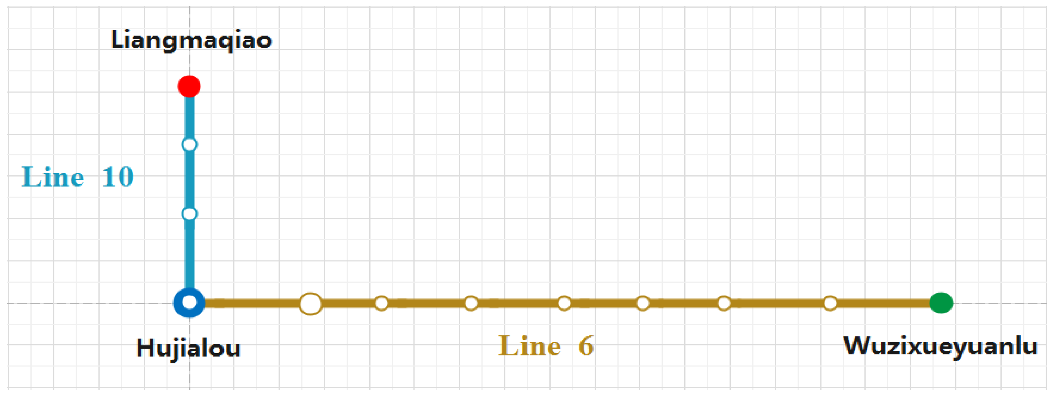
  • Segment 1: from Wuzixueyuanlu Station to Hujialou Station (Line 6, 8 stops),
  • Segment 2: from Hujialou Station to Liangmaqiao Station (Line 10, 3 stops),
as shown in Figure 3.
The data used to analyze Route A are the AFC and AVL data from 7:00 a.m. to 9:00 a.m. in ten weekdays in 2021. The auxiliary data are from:
  • Route B. from Wuzixueyuanlu Station to Hujialou Station (Line 6, 8 stops),
during the same period. The sample sizes of Route A and Route B are 2494 and 4084, respectively. Figure 4 shows the frequency histogram of Route A passengers’ tap-in and tap-out times during peak hours.
According to the data, the departure interval between two trains at Wuzixueyuanlu is about 3 min. The train travel times of segments 1 and 2 are about 21 and 6 min, respectively. The train whose departure time is 7:03 is set as Train 1 of segment 1. The first train departure interval is 7 : 00 , 7 : 03 . After removing several large outliers, we find that each passenger who enters in the interval taps out before 7:41. Therefore, all possible trains for these passengers are those shown in Table 1, which implies J = K = 3 . We can further infer that the set of all feasible itineraries is
S = { ( 1 , 1 ) , ( 1 , 2 ) , ( 1 , 3 ) , ( 2 , 2 ) , ( 2 , 3 ) , ( 3 , 3 ) }
from this table. By periodicity, this holds for all passengers whose tap-in times are from 7:00 to 9:00.

5.2. Parameter Estimation

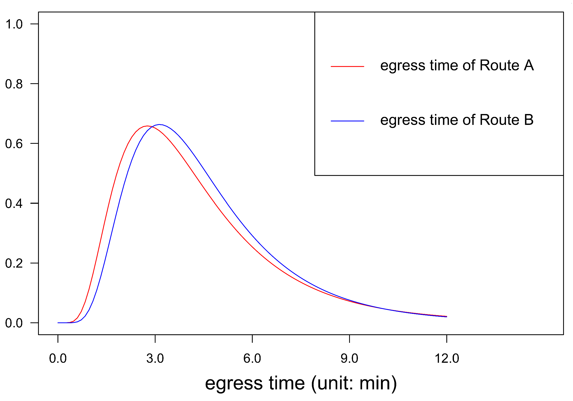
Based on the AFC and AVL data on Route A and Route B, we build the likelihood model and use the proposed EM algorithm to compute MLEs of unknown parameters. The MLEs are ( μ ^ A , σ ^ A ) T = ( 0.2329 , 0.5620 ) T and ( μ ^ B , σ ^ B ) T = ( 0.3003 , 0.5063 ) T . From this, we can get the mean and standard deviation of the distribution of egress time on Route A are 4.4346 and 0.9008 , respectively; those for Route B are 4.6047 and 0.8296 , respectively. Figure 5 shows the corresponding probability density functions. There is not much difference between the egress times on the two routes.
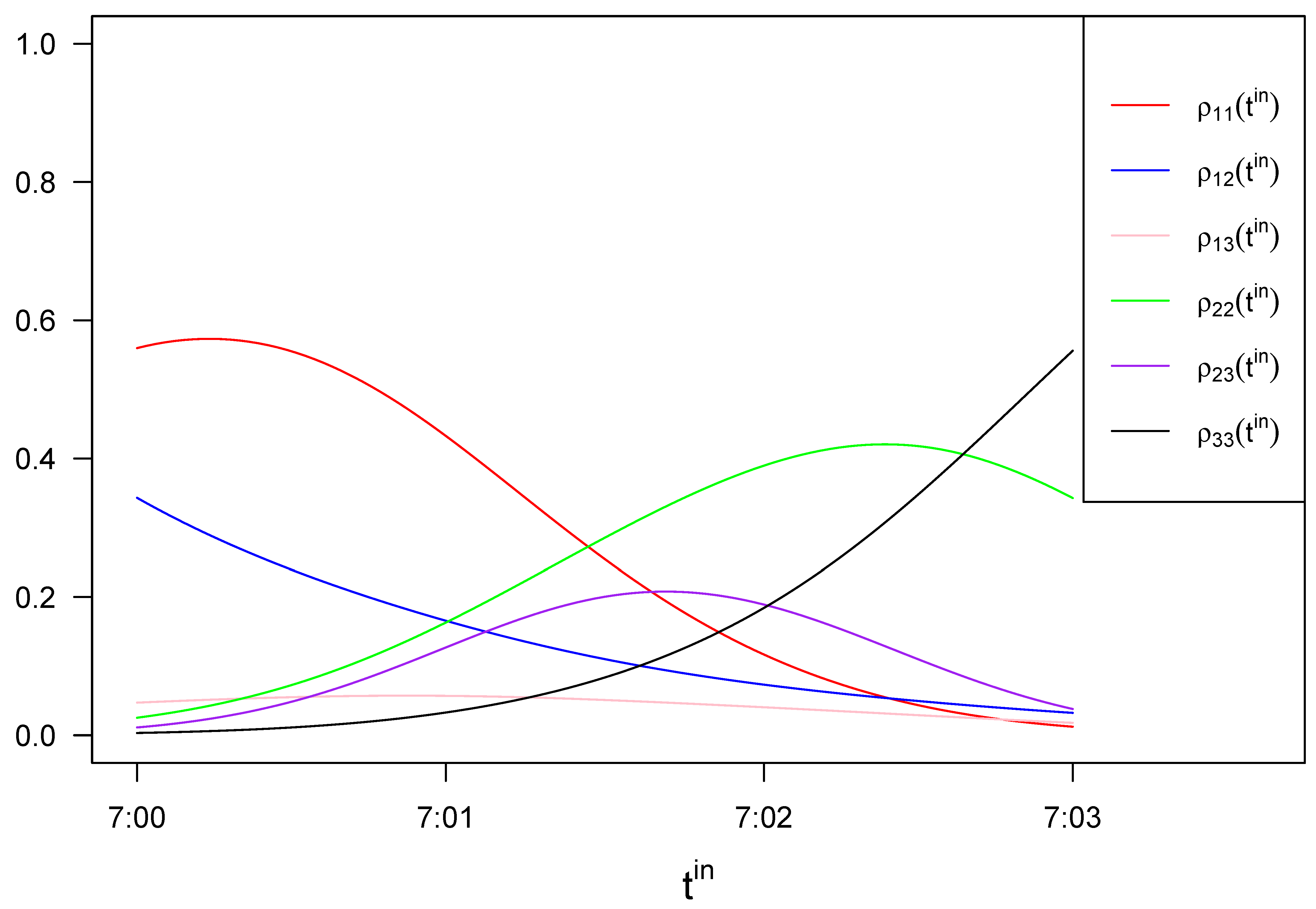
In the meantime the EM algorithm yields the MLEs of β in the logistic model (11), which further give the probabilities ρ j k ( t i n ) , ( j , k ) S in (19). Their curves with t i n varying in the first train departure interval are shown in Figure 6. It can be seen from Figure 6 that passengers are more likely to take train combinations ( 1 , 1 ) and ( 1 , 2 ) when they tap in the station earlier, and that they are more likely to take train combinations ( 2 , 2 ) and ( 3 , 3 ) when their tap-in times are closer to the train departure time. Overall, the later a passenger’s tap-in time is, the more likely he/she takes the later trains on segment 1 and segment 2. For an in-depth study, we also need to discuss the boarding probabilities and conditional boarding probabilities on segment 1 and segment 2. Curves of related boarding probabilities in (2)–(5) are presented in Figure 7. Some interesting phenomena can be found from the two figures. It can be seen from (a) and (b) in Figure 7 that, as expected, the probabilities of boarding the first (third) train on both segments 1 and 2 become smaller (larger) as t i n increases. From Figure 6, or (a) in Figure 7, we can find that passengers who tap in after 7:02 have very small probabilities of boarding the first train on segment 1. This may make the values of the conditional probabilities ρ k | 1 ( t i n ) shown by (c) in Figure 7 inaccurate. From (d) in Figure 7, the conditional probabilities ρ 2 | 2 ( t i n ) have an increasing trend as t i n goes to 7:03. A possible reason is that a passenger who enters late but boards the second train has a fast walking speed, and thus he/she has larger probability of boarding his/her first feasible train (Train 2) on segment 2. From (e) and (f) in Figure 7, we can see that the trajectories of the conditional probabilities ρ ˜ j | k ( t i n ) are consistent with our expectation. Specifically, given the train which passengers take on segment 2, we can deduce that passengers with an earlier tap-in time have a higher probability of taking Train 1 on segment 1; passengers with a later tap-in time have a higher probability of taking Train 2 or Train 3 on segment 1.
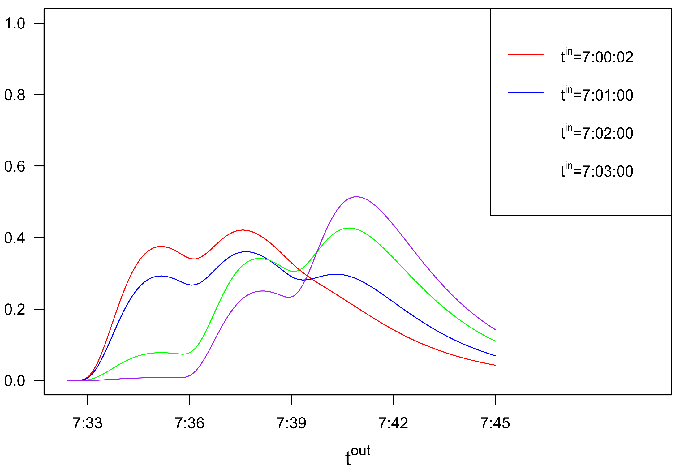
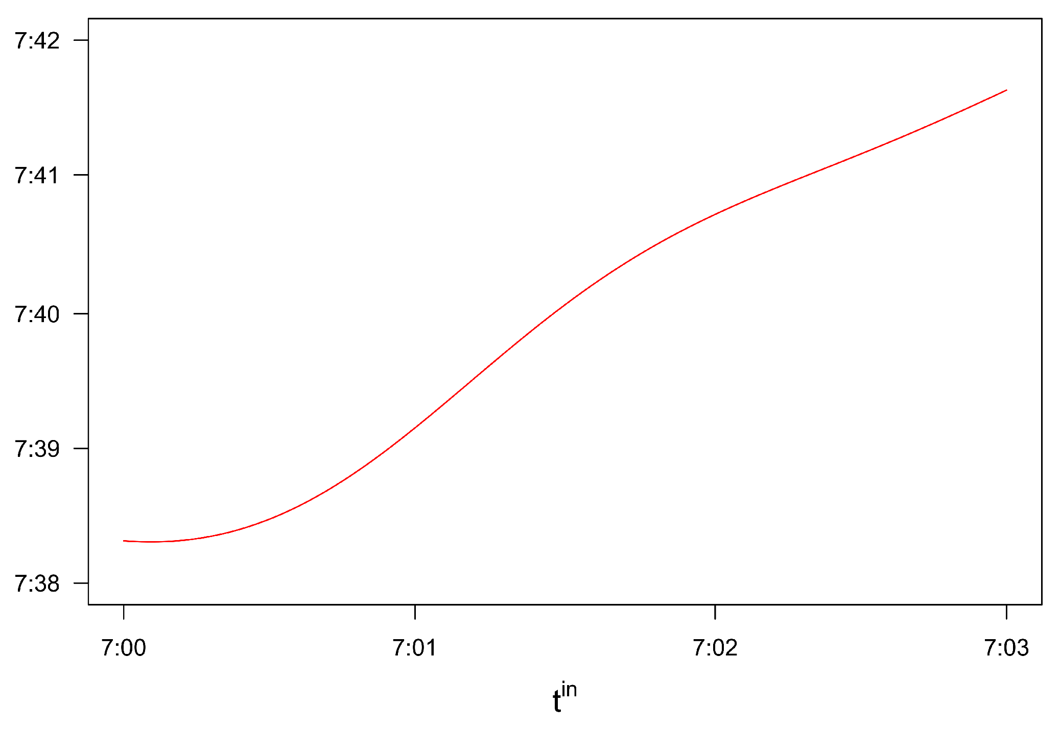
Plugging the MLEs into (6), we can get the conditional density functions of t o u t conditionally on t i n . Figure 8 presents these function curves given t i n = 7:00:02, 7:01:00, 7:02:00, and 7:03:00, respectively. They are all mixture density functions, and have more than one peak. According to (17), we can also derive the conditional mean of t o u t , shown in Figure 9. As expected, it is an increasing function with a non-linear pattern. By periodicity, it can be extended to the situation when t i n lies between 7:00 and 9:00. This curve can be used to predict the tap-out time of a passenger given his/her tap-in time.

5.3. Inference for T t r a n s f e r

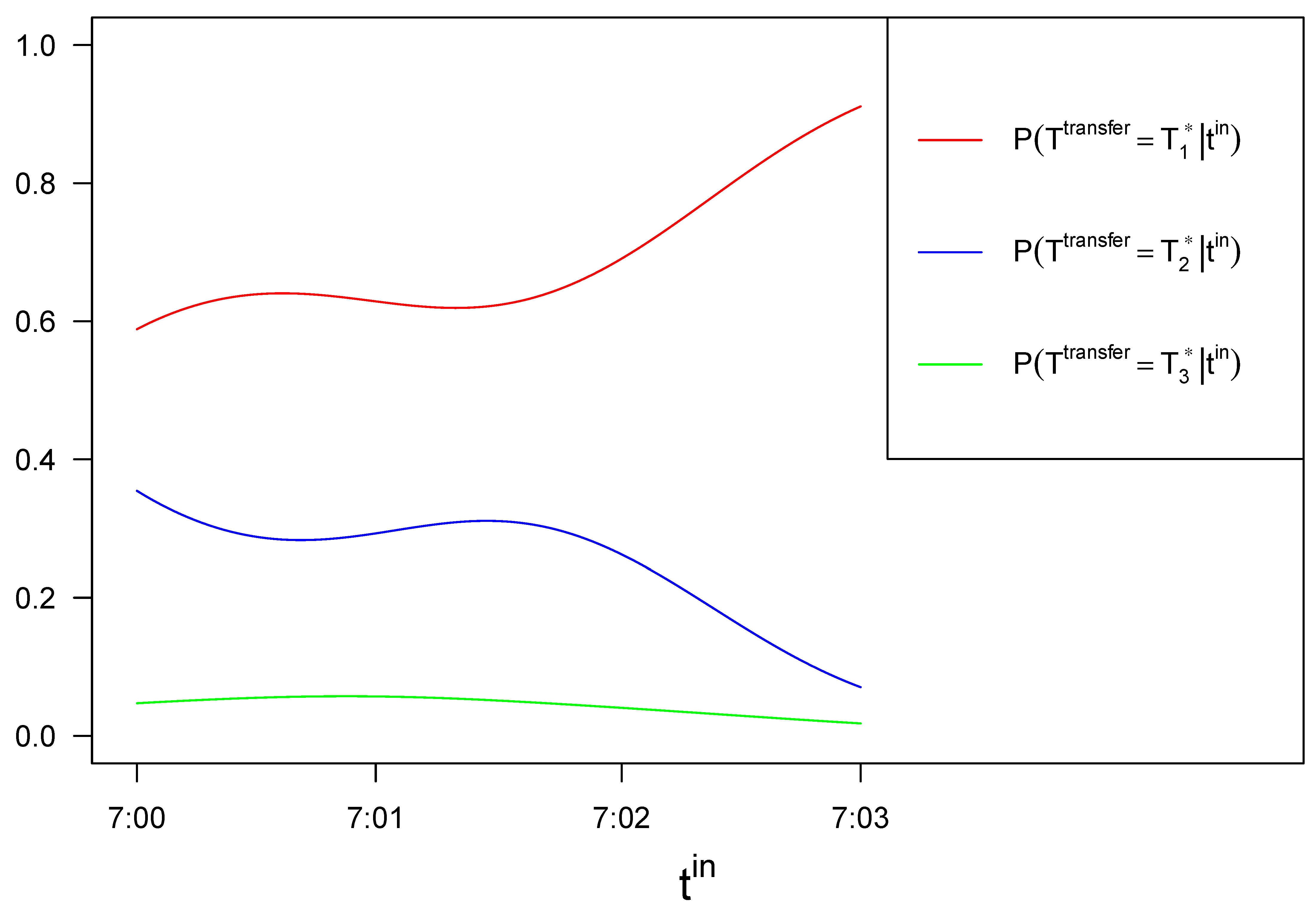
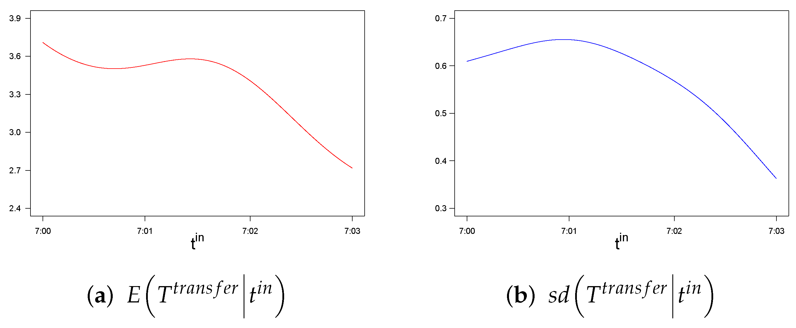
In this subsection, we infer the transfer times of passengers on Route A. First, consider the population aspect. According to Table 1, all possible values of T t r a n s f e r are in { 2.4 min , 5.4 min , 8.4 min } . Let T 1 * = 2.4 min , T 2 * = 5.4 min , and T 3 * = 8.4 min . We have P ( T t r a n s f e r = T 1 * | t i n ) = ρ 11 ( t i n ) + ρ 22 ( t i n ) + ρ 33 ( t i n ) , P ( T t r a n s f e r = T 2 * | t i n ) = ρ 12 ( t i n ) + ρ 23 ( t i n ) , and P ( T t r a n s f e r = T 3 * | t i n ) = ρ 13 ( t i n ) . Figure 10 shows the curves of P ( T t r a n s f e r = T i * | t i n ) , i = 1 , 2 , 3 with respect to the tap-in time t i n . It can be seen that, when t i n is close to 7:03, P ( T t r a n s f e r = T 1 * | t i n ) has an increasing trend. A possible reason is that, some passengers in a hurry picked up speed when seeing the train coming, and when they missed the train, they were more likely to walk fast through the transfer channel. By (12) and (13), we show the conditional mean and standard deviation of T t r a n s f e r in Figure 11. Figure 11 also indicates that the passengers whose tap-in times are close to 7:03 have a shorter T t r a n s f e r on average, which is consistent with the above inferring result. Specifically, passengers who tap in the origin station earlier are more likely to be on Train 1 of segment 1. They have less time to wait and are therefore less likely to be in a hurry to transfer, resulting in a longer transfer time. Conversely, passengers who tap in the origin station later will usually spend some time waiting for a train at the origin station, so they will have to walk faster if they want to catch Train 2 in segment 2, thus reducing their transfer times.
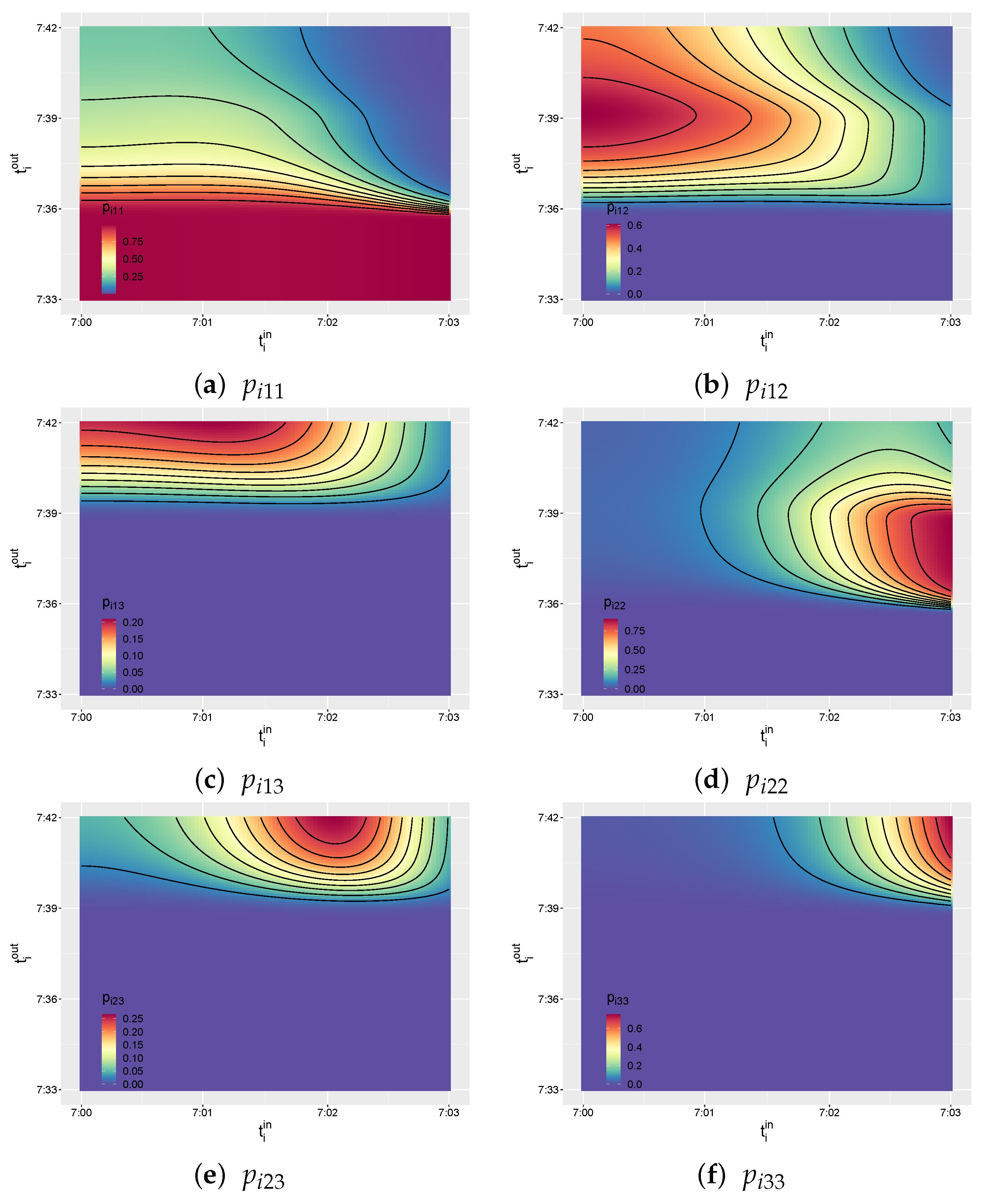
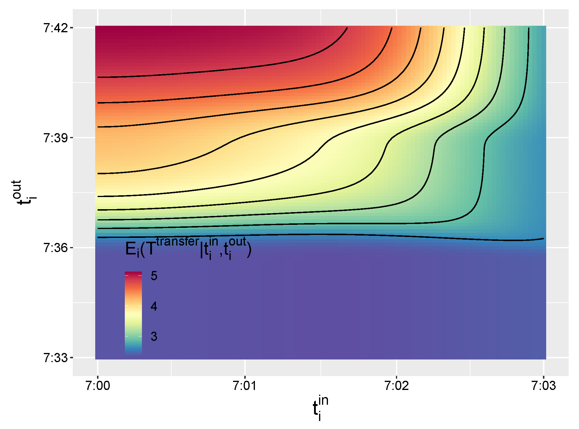
Next, consider the individual aspect. By (14), we compute the six passenger-to-train assignment probabilities p i j k , ( j , k ) S for given t i i n and t i o u t , and show their contour maps in Figure 12. Moreover, by (15), we present the contour map of the average transfer time for given t i i n and t i o u t in Figure 13. From these figures, we can infer the behavior of an individual passenger whose tap-in and tap-out times are known on the transfer route. For example, assuming that passenger i has a tap-in time of 7:02:30 and a tap-out time of 7:42:00, we can draw the conclusion of p i 11 < p i 12 < p i 22 < p i 13 < p i 33 < p i 23 from Figure 12.

5.4. Validation via CV

We use the CV method to validate the proposed model. The AFC data of passengers on Route A are randomly divided into a training set and a test set with proportions of 80% and 20%, respectively. By (18), we use the training data to construct the 95% prediction interval of the tap-out time for each tap-in time during the peak hours; see Figure 14. It can be seen that about 95% of the test data lie within the corresponding prediction intervals. This provides a validation of our model. Furthermore, an interesting phenomenon can be found from Figure 14: when a passenger’s tap-in time is close to 7:00 or 9:00, the time when the peak hours begin or end, his/her tap-out time becomes closer to the lower limit of the prediction interval. The reason is that, such a passenger has a relatively short travel time since the congestion status is not so serious at that time. We can also see that the passengers whose tap-in times lie between 7:30 and 8:30 have more even tap-out times between the upper and lower limits of the prediction interval.

6. Conclusions

This paper proposes a dynamic logistic model to study passenger flow characteristics on one-transfer metro routes. Estimates of parameters in our model can be computed by the EM algorithm based on automated AFC and AVL data. A number of passenger flow characteristics including transfer time, boarding probabilities, and travel time can be inferred and quantified with the proposed model. We also present a CV method to validate our model. Real applications to the Beijing metro show the effectiveness of the proposed model.
The proposed model and its derived inferential methods possess the following advantages. First, they are completely data-driven, with only automated data. We do not require additional information including survey data, speed information of passengers, and layouts of stations. Second, our methods provide a comprehensive analysis on passenger flow characteristics. Using reasonable statistical modeling and inferential techniques, we present quantification indices as much as possible by making full use of automated data. The obtained results can be used for the optimal management of passenger flows. For instance, we can estimate the transfer times on many transfer routes, and consider adjusting the train schedule or implementing passenger limiting at the transfer stations with long transfer times. Third, the basic idea of the dynamic logistic model is to derive the conditional distribution of a passenger’s tap-out time conditionally on his/her tap-in time. This is a very general idea, and can be followed in more complex situations.
There are several future directions:
(i)
Extensions of the proposed method to the situations where there are multiple transfers and/or multiple route selections between the origin and destination;
(ii)
Generalizations of the proposed method, possibly combined with deep learning or other machine learning methods; for analyzing the whole metro network;
(iii)
Combinations with optimization methods for improving metro management.

Author Contributions

Conceptualization, W.M. and S.X.; methodology, W.M.; software, X.W. and C.L.; validation, X.W. and C.L.; formal analysis, W.M. and X.W.; investigation, C.L.; resources X.W.; data curation, X.W.; writing—original draft preparation, W.M. and X.W.; writing—review and editing, W.M., C.L. and S.X.; visualization, X.W.; supervision, C.L.; project administration, C.L.; funding acquisition, S.X. All authors have read and agreed to the published version of the manuscript.

Funding

This work is partially supported by the National Key R&D Program of China (Grant Nos. 2021YFA1000300, 2021YFA1000301, and 2021YFA1000303) and the National Natural Science Foundation of China (Grant No. 12171462).

Data Availability Statement

Data sharing not applicable.

Acknowledgments

The authors gratefully acknowledge the editors and reviewers for their professional comments.

Conflicts of Interest

The authors declare no conflict of interest.

References

  1. Beijing Subway. Official Website. 2020. Available online: https://www.bjsubway.com (accessed on 16 September 2021).
  2. Zhang, Y.S.; Yao, E.J. Splitting travel time based on AFC data: Estimat- ing walking, waiting, transfer, and in-vehicle travel times in metro system. Discret. Nat. Soc. 2015, 2015, 1–11. [Google Scholar] [CrossRef] [Green Version]
  3. Hörcher, D.; Graham, D.J.; Anderson, R.J. Crowding cost estimation with large scale smart card and vehicle location data. Transp. Res. Part Methodol. 2017, 95, 105–125. [Google Scholar] [CrossRef]
  4. Kusakabe, T.; Iryo, T.; Asakura, Y. Estimation method for railway passengers’ train choice behavior with smart card transaction data. Transportation 2010, 37, 731–749. [Google Scholar] [CrossRef]
  5. Zhou, F.; Shi, J.; Xu, R. Estimation method of path-selecting proportion for urban rail transit based on AFC data. Math. Probl. Eng. 2015, 6, 1–9. [Google Scholar] [CrossRef] [Green Version]
  6. Sun, Y.; Schonfeld, P.M. Schedule-Based rail transit path-Choice estimation using automatic fare collection data. J. Transp. Eng. 2016, 142, 04015037. [Google Scholar] [CrossRef]
  7. Noursalehi, P.; Koutsopoulos, H.N.; Zhao, J. Real time transit demand prediction capturing station interactions and impact of special events. Transp. Res. Part C 2018, 97, 227–300. [Google Scholar] [CrossRef]
  8. Jiang, A.; Sun, Q.; Peng, Z.; Wei, X.; Huang, Q.; Tong, M. Metro OD matching and statistical research based on AFC data. J. Phys. Conf. Ser. 2020, 1624, 032051. [Google Scholar] [CrossRef]
  9. Zhu, Y.; Koutsopoulos, H.N.; Wilson, N.H.M. A probabilistic passenger- to-train assignment model based on automated data. Transp. Res. Part B: Methodol. 2017, 104, 522–542. [Google Scholar] [CrossRef]
  10. Zhu, Y.; Koutsopoulos, H.N.; Wilson, N.H.M. Inferring left behind passengers in congested metro systems from automated data. Transp. Res. Part Emerg. Technol. 2018, 94, 323–337. [Google Scholar] [CrossRef]
  11. Xiong, S.; Li, C.; Sun, X.; Qin, Y.; Wu, C.F.J. Statistical estimation for passenger-to-train assignment models based on automated data. Adv. Stoch. Model. Bus. Ind. 2022, 38, 287–307. [Google Scholar] [CrossRef]
  12. Feng, X.; Wang, X.; Zhang, H. Passenger transfer efficiency optimization modelling research with simulations. Int. J. Simul. Model. 2014, 13, 210–218. [Google Scholar] [CrossRef]
  13. Liu, X.; Huang, M.; Qu, H.; Chien, S. Minimizing metro transfer waiting time with AFCS Data using simulated annealing with parallel computing. J. Adv. Transp. 2018, 2018, 1–17. [Google Scholar] [CrossRef] [Green Version]
  14. Si, B.; He, Z.; Liu, D.; Gao, Z. Train operation diagram-based equilibrium model for an urban rail transit network with transfer constraints. J. Transp. Eng. Part Syst. 2020, 146, 04020126. [Google Scholar] [CrossRef]
  15. Wei, Z.; Fan, W.; Jin, W.; Fan, W.D. Complete estimation approach for characterizing passenger travel time distributions at rail transit stations. J. Transp. Eng. Part Syst. 2020, 146, 04020050. [Google Scholar]
  16. Zhu, Y.; Koutsopoulos, H.N.; Wilson, N.H.M. Passenger itinerary inference model for congested urban rail networks. Transp. Res. Part Emerg. Technol. 2021, 123, 102896. [Google Scholar] [CrossRef]
  17. Dempster, A.P.; Laird, N.M.; Rubin, D.B. Maximum likelihood from incomplete data via the EM algorithm. J. R. Stat. Soc. Ser. (Methodological) 1977, 39, 1–38. [Google Scholar]
  18. Liao, J.; Zhang, F.; Zhang, S.; Gong, C. A Real-Time Train Timetable Rescheduling Method Based on Deep Learning for Metro Systems Energy Optimization under Random Disturbances. J. Adv. Transp. 2020, 2020, 8882554. [Google Scholar] [CrossRef]
  19. Wu, X.; Dong, H.; Tse, C.; Zhang, Q. Timetable Synchronization Optimization for Metro Networks With the Consideration of Station Centrality. IEEE Trans. Netw. Sci. Eng. 2020, 9, 2697–2707. [Google Scholar] [CrossRef]
  20. Li, H.; Jin, K.; Sun, S.; Jia, X.; Li, Y. Metro passenger flow forecasting though multi-source time-series fusion: An ensemble deep learning approach, Appl. Soft Comput. 2022, 120, 1568–4946. [Google Scholar] [CrossRef]
  21. Li, W.; Yan, X.; Li, X.; Yang, J. Estimate Passengers’ Walking and Waiting Time in Metro Station Using Smart Card Data (SCD). IEEE Access 2020, 8, 11074–11083. [Google Scholar] [CrossRef]
  22. Hastie, T.; Tibshirani, R.; Friedman, J. The Elements of Statistical Learning: Data Mining, Inference and Prediction, 2nd ed.; Springer: New York, NY, USA, 2009. [Google Scholar]
  23. Beijing Transport Institute. Beijing Transport Development Annual Report. Beijing, China, 2020. Available online: http://www.bjtrc.org.cn (accessed on 16 February 2022).
Figure 1. Flow chart of a one-transfer metro route.
Mathematics 11 01427 g001
Figure 2. The diagram of the proposed methodology.
Mathematics 11 01427 g002
Figure 3. Transfer route from Wuzixueyuanlu Station to Liangmaqiao Station.
Mathematics 11 01427 g003
Figure 4. Frequency histograms of tap-in and tap-out times of Route A passengers in peak hours.
Mathematics 11 01427 g004
Figure 5. Density function curves of egress time.
Mathematics 11 01427 g005
Figure 6. Curves of ρ j k t i n , ( j , k ) S .
Mathematics 11 01427 g006
Figure 7. Curves of η j ( t i n ) , γ k ( t i n ) , ρ k | j ( t i n ) , and ρ ˜ j | k ( t i n ) .
Mathematics 11 01427 g007
Figure 8. Conditional density functions of t o u t conditionally on different t i n ’s.
Mathematics 11 01427 g008
Figure 9. Curve of conditional means of t o u t conditionally on t i n .
Mathematics 11 01427 g009
Figure 10. Curves of P ( T t r a n s f e r = T i * | t i n ) , i = 1 , 2 , 3 .
Mathematics 11 01427 g010
Figure 11. Curves of E T t r a n s f e r | t i n and s d T t r a n s f e r | t i n .
Mathematics 11 01427 g011
Figure 12. Contour maps of p i 11 , p i 12 , p i 13 , p i 22 , p i 23 , p i 33 .
Mathematics 11 01427 g012
Figure 13. Contour map of E i ( T t r a n s f e r | t i i n , t i o u t ) .
Mathematics 11 01427 g013
Figure 14. Prediction intervals of the tap-out times. The red and blue lines denote the lower and upper limits of the intervals, respectively. The black dots denote the test data.
Mathematics 11 01427 g014
Table 1. Train schedule.
Wuzixueyuanlu StationHujialou Station
TrainDeparture TimeArrival TimeDeparture TimeArrival Time
17:03:007:24:007:26:247:32:24
27:06:007:27:007:29:247:35:24
37:09:007:30:007:32:247:38:24
Disclaimer/Publisher’s Note: The statements, opinions and data contained in all publications are solely those of the individual author(s) and contributor(s) and not of MDPI and/or the editor(s). MDPI and/or the editor(s) disclaim responsibility for any injury to people or property resulting from any ideas, methods, instructions or products referred to in the content.