Article

Stylized Model of Lévy Process in Risk Estimation

1
Silc Business School, Shanghai University, Shanghai 200444, China
2
School of Economics and Management, Beijing University of Chemical Technology, Beijing 100029, China
3
Fundamental Technology Center, China Construction Bank Financial Technology Co., Ltd., Shanghai 200120, China
4
School of Management, Xi’an Jiaotong University, Xi’an 710049, China
5
International Business School, Shaanxi Normal University, Xi’an 710062, China
*
Author to whom correspondence should be addressed.
Mathematics 2023, 11(6), 1414; https://doi.org/10.3390/math11061414
Submission received: 20 February 2023 / Revised: 7 March 2023 / Accepted: 10 March 2023 / Published: 15 March 2023
(This article belongs to the Special Issue Planning and Scheduling in City Logistics Optimization)

Abstract

:
Risk management is a popular and important problem in academia and industry. From a small-scale system, such as city logistics, to a large-scale system, such as the supply chain of a global industrial or financial system, efficient risk management is required to prevent loss from uncertainty. In this paper, we assume that risk factors follow the Lévy process, and propose a stylized model, based on regression, that can estimate the risk of a complicated system under the framework of nest simulation. Specifically, portfolio risk estimation using the Lévy process is discussed as an example. The stylized model simplifies the risk factors artificially, and provides useful basis functions to fit the portfolio loss with little computational effort. Numerical experiments showed the good performance of the stylized model in estimating risk for the Variance Gamma process and the Normal Inverse Gaussian process, which are two examples of the Lévy process.

1. Introduction

Risk management is of great importance for the modern business environment. Risk estimation or evaluation is always an attractive and challenging problem in management science. For example, in supply chain management or project management, risk estimation is always the very first step of the risk management of the system to be analyzed [1,2,3]. In the field of finance, risk measures of portfolios, as well as of the financial market, are two classical, but difficult, topics discussed in financial risk management [4,5].
To the best of our knowledge of related literature on risk measures, several widely applied frameworks of risk measures are proposed [6,7,8]. According to the results shown in [6], some papers try to measure risk by probabilistic or scenario approaches in supply chain risk management to analyze uncertainty. Similarly, risk measures, like Value-at-Risk (VaR), Exceedance probability and Expected shortfall (ES), are usually used to measure the risk of one portfolio or of the financial system [9]. These measures are basically designed under a related system with uncertainty, which is seen as the source of risk. However, the measurement of one system’s risk is difficult because there are multiple risk factors (sources of risk) that affect the whole large system. These risk factors may be propagated, or amplified, by the system. This makes risk measurement harder in a large system. When the analytical form of risk measure is out of hand, several estimation methods are proposed to estimate the risk measures for the system. Basically, the Monte Carlo simulation (MC) provides a useful tool to estimate risk measure and can be applied by most systems without specific constraints. So there is a stream of related literature estimating risk under the framework of the Monte Carlo simulation [10,11]. Usually, MC generates the possible scenarios of risk factors in the future and calculates potential loss under each scenario. Among them, the nested simulation framework, proposed by [12], is purported to simulate the risk factors between any future time intervals, and evaluates the corresponding loss of a system to measure the risk. Basically, nested simulation includes the outer simulation, that generates multiple scenarios of risk factors, and the inner simulation, that generates and calculates the possible system loss in each scenario. It builds up the framework of risk estimation for a system. However, it also encounters trouble in a huge system problem because the required computational effort is too large to obtain reliable results. To solve this problem, related literature discusses the balance of computational effort between outer simulation and inner simulation. Furthermore, some papers, such as [12,13,14,15], have tried to improve the estimation efficiency or accuracy.
One marked stage of improvement comes from [16]. This paper considered portfolio risk estimation in financial engineering and used regression to fit the surface of portfolio loss, given the risk factors. Several papers proposed related models based on this framework [17,18]. The risk estimation via regression can relax the computational requirement by substituting the inner simulation by a pre-trained regression. Of course, because of the complexity of a system, the performance of risk estimation via regression is problem-dependent and the selection of basis function is of great importance. Intuitively, the appropriate selection of basis function becomes harder for complicated portfolios, such as a portfolio with several derivatives trading in the financial market, because there exists high non-linearity in this system (portfolio) with respect to risk factors [19,20].
In this paper, we discuss the risk estimation problem under the framework of portfolio risk management and focus on the basis function selection problem in risk estimation via regression. Portfolio risk management with a complicated structure (including special financial products, such as derivatives) can be a good example of the complex systems we are interested in. Furthermore, we considered a portfolio having risk factors following the Lévy process, which is a type of more generalized stochastic process that has become a newly applied modeling perspective in finance and many other fields. Instead of the polynomial basis function, that is supported by the theory of functional analysis and widely used in the existing literature, we propose a stylized model that is derived by considering artificially simplified risk factors, coupled with the closed form of derivative price. We argue that portfolio loss with simplified risk factors can explain, or cover, the non-linearity of portfolio loss under the Lévy process in most cases. The simplified loss is easy to derive and can be selected as the basis function. Finally, we describe the related methods to test the efficiency of the stylized model and examine the performance of the stylized model in numerical examples.
This paper is organized as follows. In Section 1, we give a brief introduction of the background and related literature. The stylized model proposed in this paper is illustrated in Section 2, including the efficiency testing of the proposed model. Section 3 designs the numerical example to show the performance of the proposed model. Section 4 concludes this paper and shows the potential future research.

2. Model Setting

In this paper, we are interested in estimating the risk measures of complicated portfolios. Based on the nested simulation framework in [12], and inspired by [16], we further propose a stylized model that considers the risk factors following the Lévy process.

2.1. Nested Simulation

Consider a complicated portfolio that may contain multiple financial derivatives, such as futures, options, etc. We call the underlying assets that affect the price of these derivatives the risk factors. The vector of risk factors is denoted as ω Ω and Ω is the state space of vector of risk factors. The Value Φ ω ( 0 ) is the portfolio value at time 0, which can be observed in the real world. Let Φ ω ( τ ) be the valuation of portfolio at time τ ( 0 , T ] and T be the end of the portfolio life period. The portfolio loss between risk horizon 0 to τ is defined as
L ω ( τ ) = Φ ω ( 0 ) Φ ω ( τ ) .
Then, any risk measure for the portfolio can be defined as a function f of portfolio loss
Risk Measure = E [ f ( L ω ( τ ) ) ] .
We consider risk measures of portfolios with different f commonly used in real application. For instance, we consider the probability of large loss can be defined as P ( L ω ( τ ) > q ) , where q > 0 is a given constant. Then, VaR α is the 1 α quantile of portfolio loss that is defined as inf { q : P ( L ω ( τ ) > q ) α } . Expected shortfall (ES) is the expectation of portfolio loss on condition that the event’s portfolio loss exceeds the corresponding VaR, E ( L ω ( τ ) | L ω ( τ ) > VaR α ) .
The risk factors can be observed at time 0 but the loss of portfolio depends on the dynamics of risk factors in the future, which is unobserved. Usually, V ω ( τ ) and V ω ( 0 ) cannot be determined analytically, or calculated directly, at times τ and 0, because the value of this portfolio may be determined by possible payoff in the future. Take the European call option as the simplest example, wherein an analytical formula for risk factors is not available following the majority of stochastic processes. Instead of deriving the closed form of portfolio loss distribution, Monte Carlo simulation [21] provides an useful tool to generate the possible scenarios of portfolio loss L ω ( τ ) , and estimates the corresponding risk measures. Based on the framework of Monte Carlo simulation, the nested simulation framework, proposed by [12], estimates risk measures and is widely applied in financial engineering and risk management.
Figure 1 shows the structure of nested simulation. It includes the “outer simulation” and “inner simulation”. The parameters n and m determine the sample size of risk factors that need to be generated in the “outer simulation” and “inner simulation”, respectively. The “outer simulation” generates n risk factors at time τ , based on observed risk factors at time zero. For each set of simulated risk factors in the “outer simulation”, the “inner simulation” generates the m possible outcomes of the risk factor ω from τ to T. Each possible outcome of risk factors after time τ can help in evaluating the value of the portfolio at τ . If the value of the portfolio at time τ is path-dependent, such as the Asian option and the barrier option, the “inner simulation” may simulate m path of risk factors from time t to T, instead of possible outcomes of risk factors at time T. Figure 1 only shows the example that generates the possible realizations of risk factor at time T.

2.2. Stylized Model in Lévy Process

In nested simulation, the dynamics of risk factors considered may be of great importance. Take the stock options in our portfolio as an example, the classical Black–Scholes (B–S) model assumes that the underlying stock follows the geometric Brownian motion. Then, it can show the analytical formula of the European option price by Itó’s lemma. However, empirical evidence suggests that the B-S model cannot fully describe the statistical properties of financial time series or risk factor, which is actually a Markov process. The non-Gaussian character is usually observed in financial time series in the real world and the geometric Brownian motion can only model fixed volatility instead of stochastic volatility.
Inappropriate assumptions on risk factors absolutely affect the performance of estimated risk measures in real applications. In this paper, we consider a more generalized assumption on risk factors. We assume that the risk factors, such as stock prices, commodity prices, interest rate, and foreign exchange rate, follow the Lévy process. Compared with Geometric Brownian motion, the Lévy process is a more general stochastic process that also has independent and stationary increments [22]. Based on this assumption, we can still apply nested simulation to estimate the risk measure with the following procedures.
  • Outer simulation: Given the vector of risk factors ω ( 0 ) , simulate n risk factors at time τ from the Lévy process, denoted as the design points.
    { ω 1 ( τ ) , ω 2 ( τ ) , , ω n ( τ ) } .
  • Inner simulation: For each ω i ( τ ) , simulate m risk factors at time T from Lévy process, denoted as
    { ω i 1 ( T ) , ω i 2 ( T ) , , ω i m ( T ) } .
    For each path ω i ( τ ) ω i j ( T ) , we calculate the portfolio loss
    L ^ ω i j ( τ ) = Φ ω ( 0 ) Φ ^ ω i j ( τ ) ,
    where i = 1 , 2 , , n and j = 1 , 2 , , m . For instance, if a portfolio only contains one European call option and the risk factor is the underlying stock price, we have Φ ^ ω i j ( τ ) = e r ( T τ ) ( ω i j ( T ) K ) + , where ω i j ( T ) is the jth stock price observation simulated from the Lévy process, given stock price ω i ( τ ) at time τ .
    The estimated portfolio loss for each path is
    L ¯ ω i ( τ ) = 1 m j = 1 m L ^ ω i j ( τ ) ,
    where i = 1 , 2 , , n .
  • Estimate the risk measure in Equation (2) by
    Risk Estimator = 1 n i = 1 n f L ¯ ω i ( τ ) .
Remark 1. 
In the nested simulation procedures above, we assume that Φ ω ( 0 ) is known, because the value of the portfolio may be observed in the real market at time 0. One may still need to estimate it via the Monte Carlo simulation if that is not the case.
The estimation precision of the risk measure above could be determined in two parts: outer simulation sample size n and inner simulation sample size m. We can obtain a good estimation of portfolio loss if m is sufficiently large, and a good estimation of risk measure based on the portfolio loss if n is sufficiently large. The appropriate setting of n is usually dependent on function f. However, when we consider a portfolio with thousands of financial products, m becomes too large to reach a good estimation of portfolio loss. To solve this problem, ref. [16] proposes that one may use regression to fit the portfolio loss, then provide a portfolio loss function that can reduce the computational efforts. Specifically, let a set of real-valued functions Ψ ( ω ) = ψ 1 ( ω ) , ψ 2 ( ω ) , , ψ d ( ω ) be the basis function of the portfolio loss function L ( ω ) , where ω Ω . We are interested in finding a vector of coefficient r R d such that
L ( ω ) Ψ ( ω ) r + ϵ ( ω )
In general, there are always some generic choices of basis functions Φ ( ω ), such as polynomials. Ref. [16] also recommends some selection of basis functions from the payoff function. In this paper, we propose a stylized model that chooses better basis functions for portfolios when risk factors follow the Lévy process, instead of Geometric Brownian Motion (GBM). Take a portfolio with one call option as an example. The vector of risk factors ω is the stock price at maturity and strike price is K. Let C B S ( ω ) be the call option price with underlying stock following the GBM, which can be calculated by the Black–Scholes model. We can consider the following seven basis functions for comparison:
  • Basis 1: 1, C B S ( w ) (Stylized model)
  • Basis 2: 1, ω , ω 2 (Polynomials)
  • Basis 3: 1, ω , ω 2 , C B S ( w )
  • Basis 4: 1, ω , ω 2 , ω 3
  • Basis 5: 1, ω , ω 2 , ( ω K ) + (Polynomial + Payoff)
  • Basis 6: 1, ω , ω 2 , ( ω K ) + , ( ω K ) 2 , C B S ( w ) (Polynomial + Payoff + Stylized model)
  • Basis 7: 1, ω , ω 2 , ( ω K ) + , ( ω K ) 2 , ω 3
Basis 1 is called the Stylized model. For constant term, we only choose C B S ( ω ) as the basis function. The close form of option price is easy to obtain if we assume that the underlying stock follows GBM. If we try to match the related features of stock to the corresponding parameters of GBM, the true option price can be roughly estimated by C B S ( ω ) . Then one can get the basis function (Basis 1), which is easy to calculate and highly related to the true option value. Basis 2 and Basis 4 are widely used polynomials. Due to the non-linearity between stock price and option price, here we consider the higher order polynomial function instead of one. Values ( ω K ) + and ( ω K ) 2 in Basis 5 through to Basis 7 are recommended in [16], that used the payoff function as its basis function, which also showed good performance in their numerical experiments. It is reasonable that we set Basis 3 through to Basis 5 in one group and Basis 6 and Basis 7 in another as two separated groups, because there are the same numbers of basis functions in each group. Intuitively, the stylized model works well for appropriate parameter setting so that GBM can roughly approximate the Lévy process. So, we propose the parameter adjustment rule in the stylized model. That is,
Volatility of stock price follows the L é vy process = Volatility of stock price follows GBM .
Remark 2. 
Stylized model for general case.
The stylized model is easy to obtain for most of the cases in complicated large portfolios. For instance, the option prices formula is usually easy to obtain under the GBM framework, such as the B–S formula for basket option, Asian option, and barrier option. For some other exotic options, one may simplify the underlying stock from the Lévy process to GBM, as well as option payoff from exotic options to simple European option. Then, one can obtain the close form of simplified option price as the basis in the stylized model.
Remark 3. 
The usefulness and efficiency testing of Stylized Model.
To test the usefulness of the stylized model as the basis function of regression, we designed the following hypothesis testing with null hypothesis H 0 and alternative hypothesis H 1 ,
H 0 : r = 0 . H 1 : r 0 .
Here, one can use Z-test to test the efficiency of the stylized model. For efficiency of the stylized model, K 2 statistics and AIC, BIC can also be used to evaluate goodness of fit. See [23] for details.

3. Numerical Examples

In this section, we describe the four numerical examples we designed to examine the performance of the stylized model in estimating the risk measure. Still, we assumed that the underlying assets of financial derivatives follow the Lévy process and used the European option as the example of derivatives. So the underlying asset price at time t, denoted as S t , is the vector of risk factors in this example. Take the Variance Gamma (VG) process and the Normal inverse Gaussian (NIG) process as the dynamics of the derivatives’ underlying assets. We considered the following four portfolios in Table 1 and Table 2. In each numerical example, we evaluated the estimation performance of Value-at-Risk (VaR) by different choices of basis function. VaR of any random variable X given α , denoted as VaR α , is defined as
Pr { X VaR α } = α .
Suppose that the initial prices of underlying assets are denoted by S 0 , risk-free interest rate r = 2 % , and the maturity of all options T = 1 . The risk horizon is τ = 0.25 year. There are 4 portfolios considered and each of them consists of one long European call option with underlying assets S 1 and strike price K 1 , one short European call option with underlying assets S 2 and strike price K 2 , and one short call option with underlying assets S 3 and strike price K 3 . The parameters of options in portfolios are shown in Table 1. The parameters of underlying assets are shown in Table 2.
Given the parameters setting above, we built our experiments, including the following two procedures. The first part is the training procedure. Given α , we replicated our numerical experiment H = 1000 times. For each replication, let M be the number of sample paths of risk factors we generate in the outer simulation for each replication. Here, we set M = 500, 5000, 50,000, 100,000, respectively. For inner simulation, we set the number of simulation paths as m = 1 . Therefore, we have M sample paths, or scenarios. So, the corresponding portfolio loss in i-th scenario, L ^ ω i 1 , which is the element of L ( ω ) in Equation (3) can be computed. The basis functions Ψ ( ω ) are selected according to the description of Basis 1 through to Basis 7. The parameter r can be estimated by ordinary least square (OLS), given the portfolio loss and basis, denoted as r ^ . The second part is the testing procedure. Set testing sample size N = 10,000; that is, we generated N scenarios for each replication to calculate basis. Given the r ^ , we can estimate the portfolio loss. Then, the risk measures VaR ^ α h can be estimated, h = 1 , 2 , , H . The true values of VaR are not available in these numerical examples. We used nested simulation to estimate them. The computational budgets for α = 0.95 , 0.99 , 0.995 were 10 6 , 10 7 , and 10 8 .
The stylized model assumes that the underlying assets follow the Geometric Brownian Motion (GBM) with estimated volatility. Here we may have two ways to estimate it in the numerical examples. Firstly, one can calculate the volatility of the Lévy process to match the one in GBM. For example, consider the VG process as an example, its variance σ V G 2 = ( σ 2 + ν θ 2 ) . The calculation is straightforward for the stochastic process with independent increment. Alternatively, we can estimate the volatility from the simulated underlying asset price. This is widely applied in real applications. According to [24], given n samples of underlying asset price at time T, ω T = { S T 1 , S T 2 , , S T n } , the volatility σ G B M in GBM can be estimated by the following procedure:
σ ^ G B M = s T , s = 1 n 1 i = 1 n ( u i u ¯ ) 2 , u i = ln S T i S 0 .
where u ¯ = i = 1 n u i / n .
For evaluation and comparison of estimation performance using different basis functions, we calculated the relative root mean square error(rRMSE) to show the results in Table 3, Table 4, Table 5 and Table 6. The rRMSE is calculated using the following equation:
rRMSE = h = 1 H ( VaR ^ α h VaR α ) 2 H × VaR α .
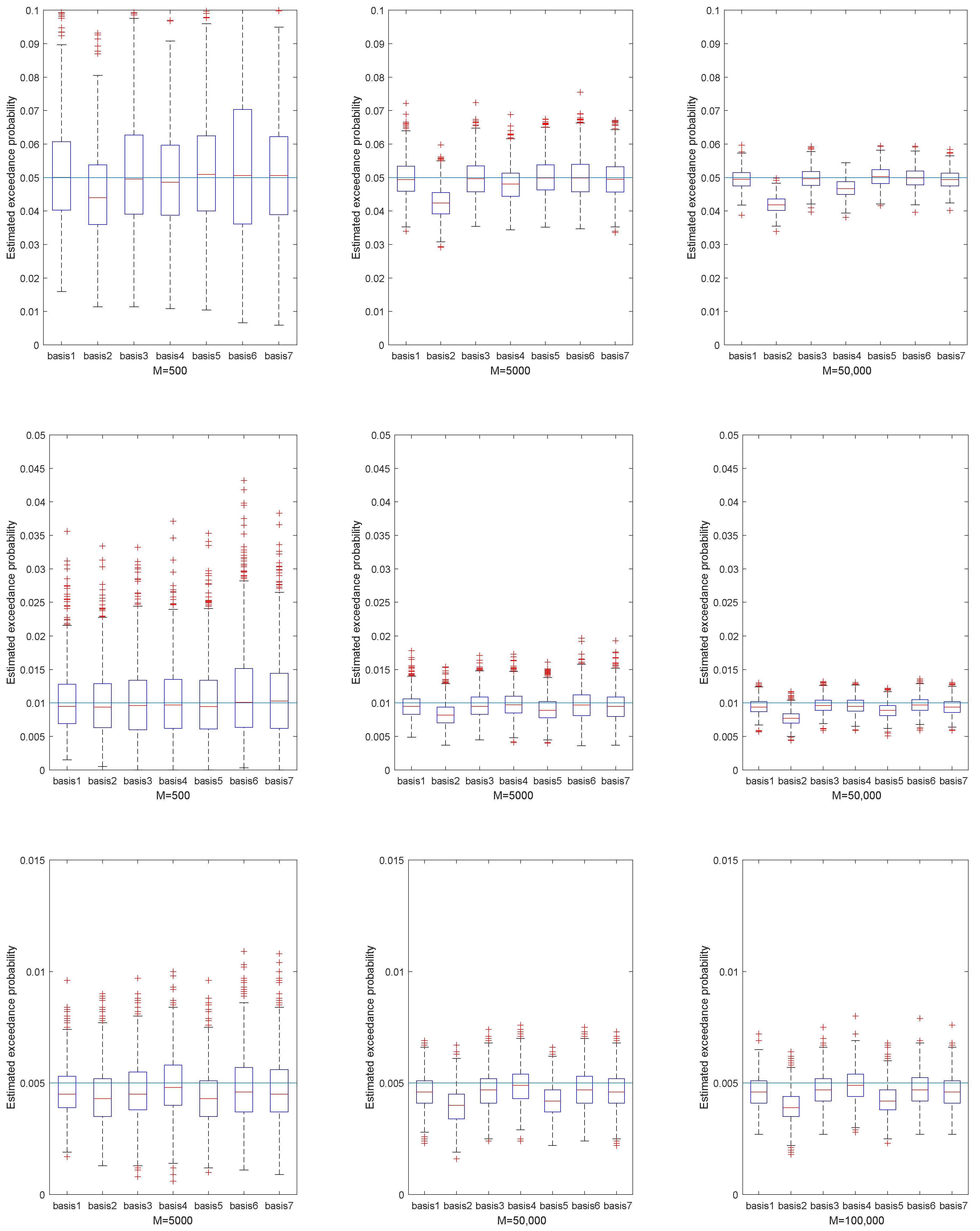
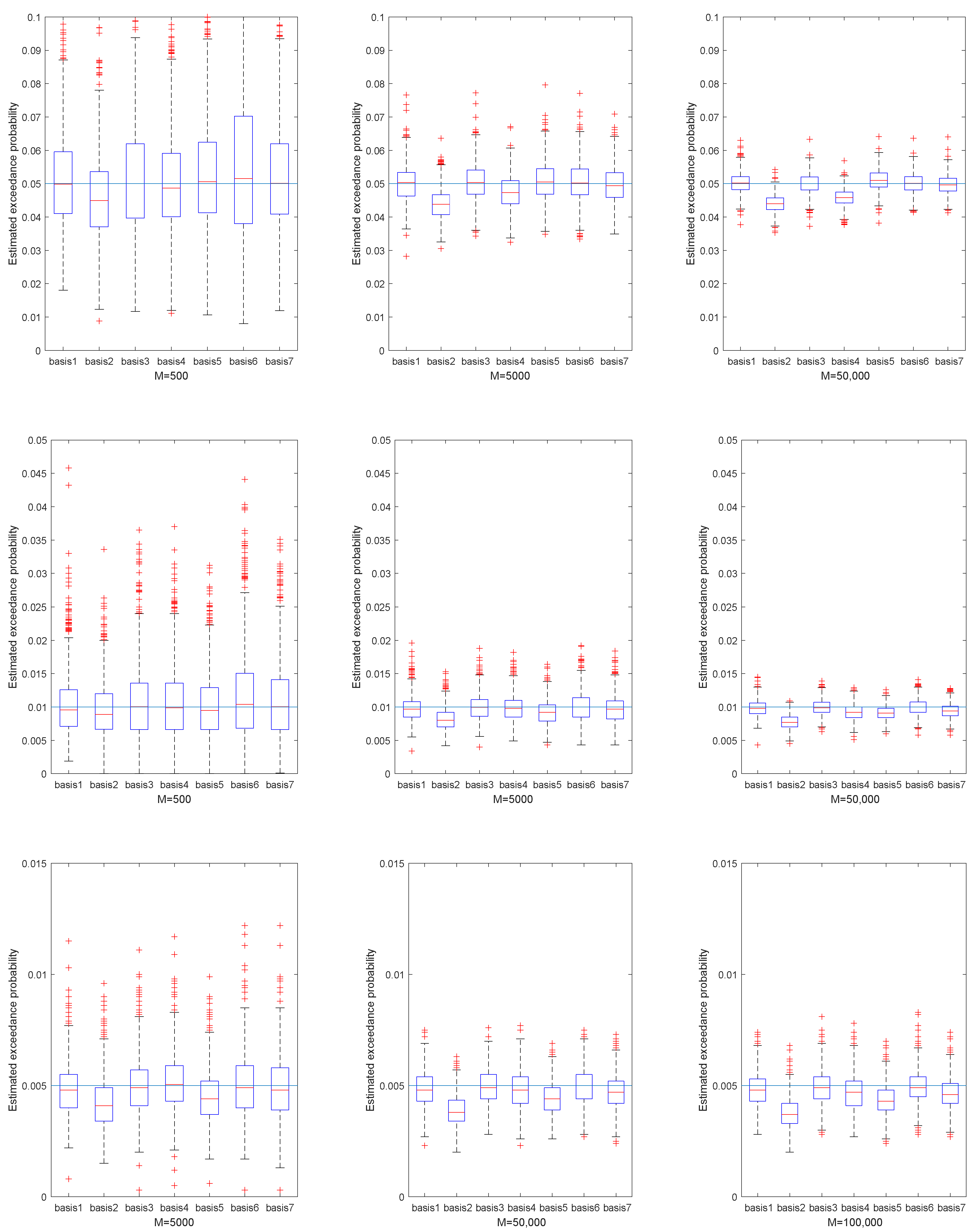
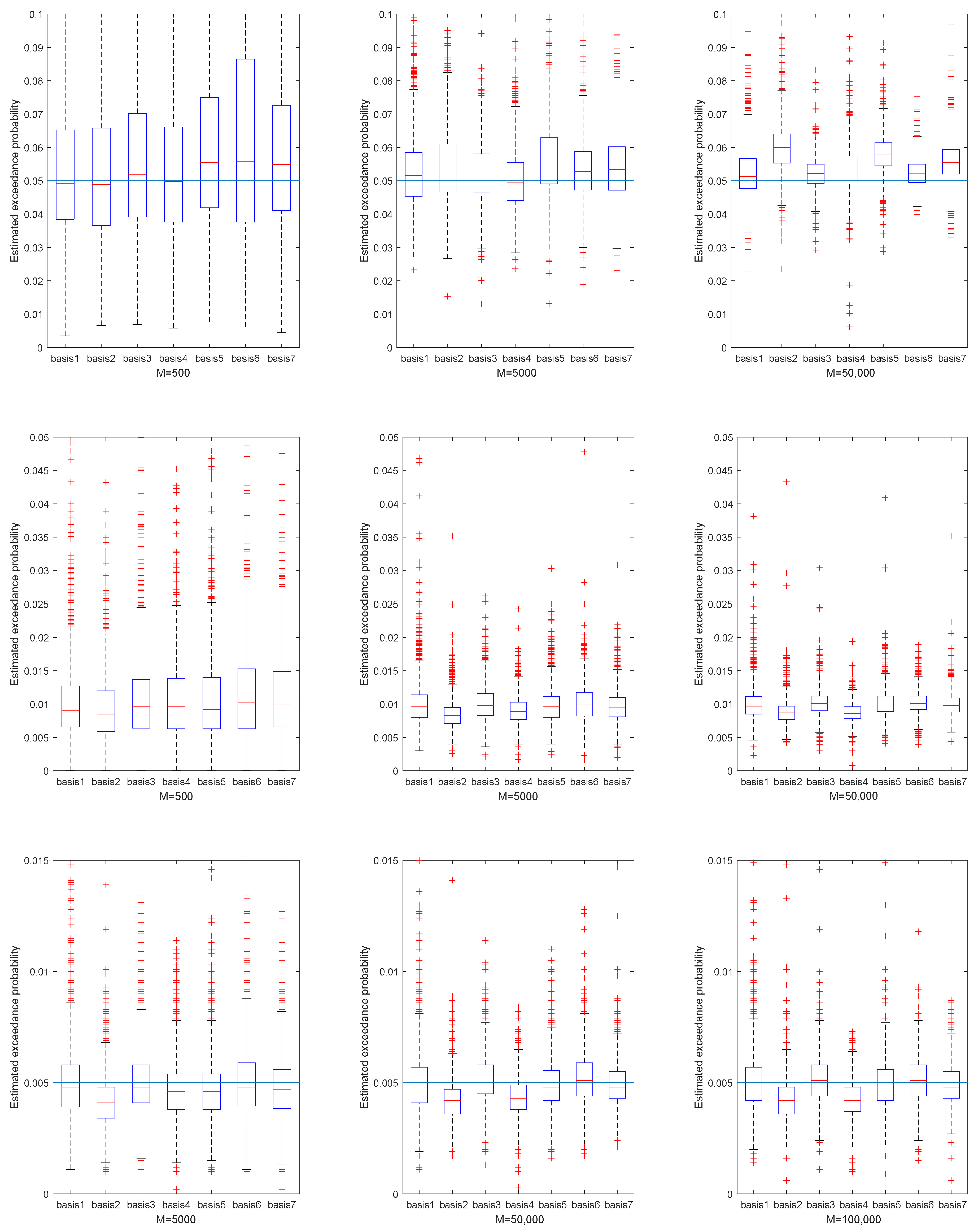
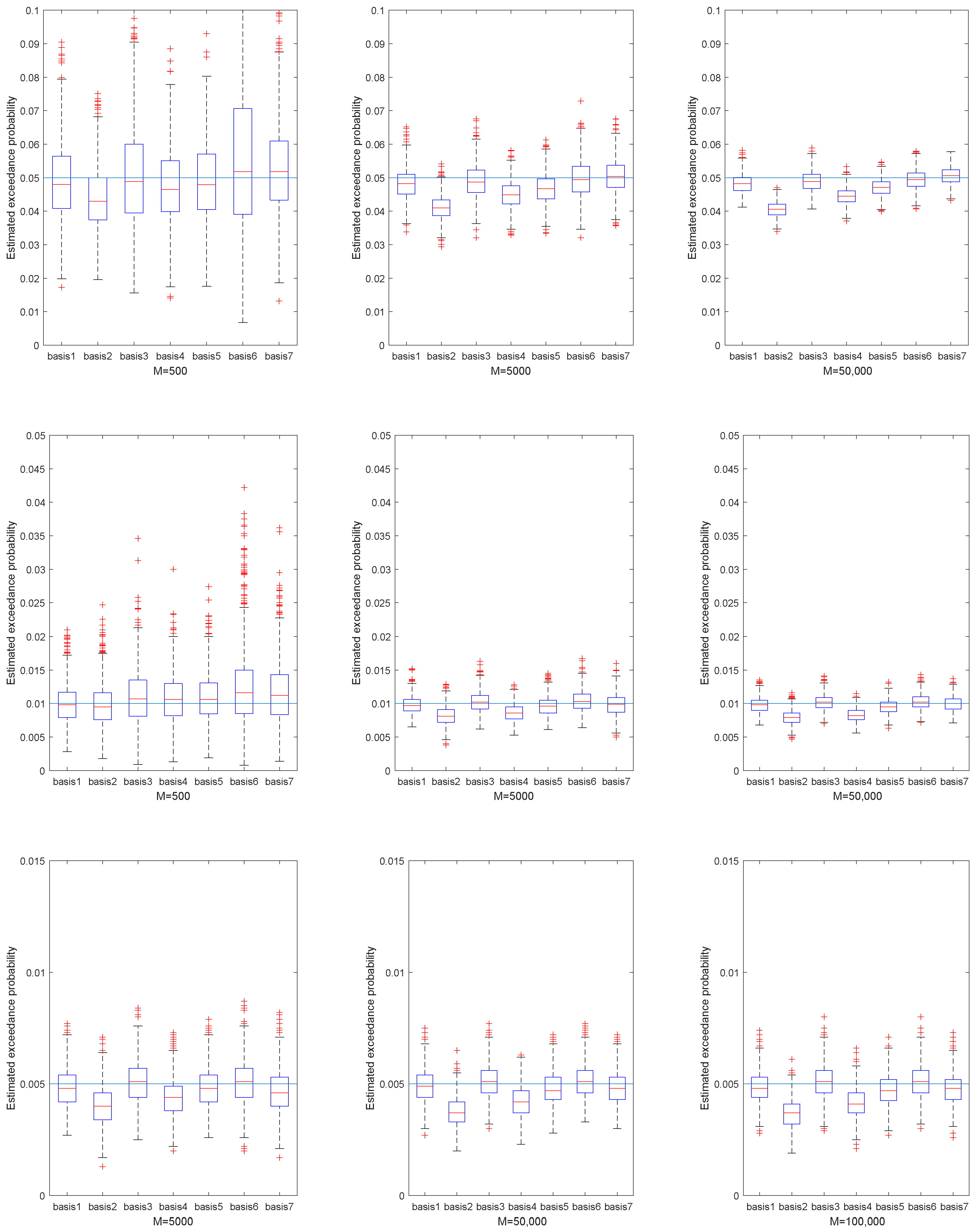
Furthermore, we show the box plot of exceedance probability of estimated VaR in Figure 2, Figure 3, Figure 4 and Figure 5 for each replication, defined as
Exceedance Probability = 1 N i = 1 N 1 { L ^ ω T i 1 VaR α } .
Table 3, Table 4, Table 5 and Table 6 show the rRMSE of estimated VaR α , where α = 0.95 , 0.99 , 0 , 995 , respectively. Seven different basis functions were tested in the experiments. In general, the estimation became harder if α increased, given the fixed sample budget in the training parts for all the basis functions. So, all the tables show that the rRMSE increased as α increased in most cases. For comparison, 7 basis functions were divided into three groups with similar lengths. The rRMSE with the blue color was the best basis, based on the rRMSE of estimated VaR . Group 1 consisted of Basis 1 and Basis 2. Basis 1 is the simplest stylized model that only contains the first-order term of B–S price. Basis 2 contains both the linear term and the second-order term of risk factors to capture the high non-linearity of portfolio loss with respect to risk factor. A basis function with only a linear term of risk factors showed really bad performance in all settings, so we excluded it. Group 2 consists of Basis 3, Basis 4, and Basis 5. All the basis functions were designed based on Basis 2 and another different basis function. Basis 3 considers the stylized model. Basis 4 considers the higher order of risk factors. Basis 5 was designed according to [16]. Inspired by the payoff function of European call option, it tries to capture the non-linearity by ( S T K ) + . Group 3 consists of Basis 6 and Basis 7, in order to evaluate the estimation performance of higher order basis functions.
As these tables show, basis functions with the stylized model (Basis 1, Basis 3 and Basis 6) performed better than others in most cases. Furthermore, if we compare each group, the basis function with the stylized model performed better. For comparison among groups, the basis functions ( S T K ) + (Basis 5 and Basis 7) were worse than the basis function with the stylized model, but much better than the polynomial basis functions (Basis 2 and Basis 4). Specifically, the estimation performance was surprisingly good with only one stylized model ( C B S ( S T ) ). Except for portfolio 3, all rRMSEs were around 0.15%. Meanwhile, little improvement was shown in Basis 3 and Basis 6, compared with Basis 1, in some portfolios. For example, there was nearly no improvement of Basis 3, compared with Basis 1, in portfolio 2 with α = 0.95 , and 0.004% improvement of Basis 5, compared with Basis 1. This also shows the efficiency of the stylized model as basis function in regression Equation (3).
Figure 2, Figure 3, Figure 4 and Figure 5 represent the estimated exceedance probability, given estimated VaR , in the four portfolios, respectively. The red line of each box plot is the median of estimated VaR in H replications. The light blue line is the true exceedance probability. As the training sample increased from M = 500 to M = 50,000 for α = 0.95 , 0.99 , and from M = 5000 to M = 100,000 for α = 0.995 we see better estimation results of exceedance probability. Specifically, the estimation results in Figure 4 fluctuated much more than in Figure 5, because the underlying NIG process had larger variance. So, estimating the VaR in portfolio 3 was relatively harder than in portfolio 4. Similarly, if we compare the median of estimated exceedance probability, the basis with the stylized model performed better than the others. Still, we did not observe large improvement from Basis 3 and Basis 5 compared to Basis 1 in most cases.

4. Conclusions

In this paper, we proposed a stylized model that deals with the risk estimation problem in complicated and large portfolios. The stylized model is based on nested simulation and regression. Specifically, we considered a complicated portfolio with risk factors following the Lévy process and used the Black–Scholes formula as the basis function in the stylized model. The usefulness and efficiency testing are discussed. The numerical results showed better performance of the stylized model compared with the basis functions inspired by polynomial basis and the payoff function. In general, the stylized model can be widely applied to estimate portfolio risk with a limited computational budget. In future research, one potential field may be to consider a very large portfolio, such as a portfolio with hundreds of derivatives and assets. Another possible future consideration could be an alternative portfolio risk estimation procedure, instead of regression, such as the surface fitting model, including stochastic kriging.

Author Contributions

Conceptualization, X.Y., Y.Y., H.L. and Y.L.; Formal analysis, X.Y.; Investigation, X.Y.; Methodology, X.Y., Y.Y., H.L. and Y.L.; Resources, K.-K.L.; Supervision, K.-K.L.; Writing—original draft, X.Y.; Writing—review & editing, Y.Y. and K.-K.L. All authors have read and agreed to the published version of the manuscript.

Funding

This research was funded by the National Natural Science Foundation of China, grant number 72201161 & 72103017.

Data Availability Statement

Not applicable.

Acknowledgments

We are grateful to Jeff L. Hong (Fudan University) and Guangxin Jiang (Harbin Institute of Technology) for the constructive comments that significantly helped to improve this paper.

Conflicts of Interest

The authors declare no conflict of interest.

References

  1. Ho, W.; Zheng, T.; Yildiz, H.; Talluri, S. Supply chain risk management: A literature review. Int. J. Prod. Res. 2015, 53, 5031–5069. [Google Scholar] [CrossRef]
  2. Gurtu, A.; Johny, J. Supply chain risk management: Literature review. Risks 2021, 9, 16. [Google Scholar] [CrossRef]
  3. de Araújo Lima, P.F.; Crema, M.; Verbano, C. Risk management in SMEs: A systematic literature review and future directions. Eur. Manag. J. 2020, 38, 78–94. [Google Scholar] [CrossRef]
  4. Hopper, G.P. Value At Risk: A New Methodology for Measuring Portfolio Risk. Business Review, July 1996, pp. 19–31. Available online: https://www.philadelphiafed.org/-/media/frbp/assets/economy/articles/business-review/1996/july-august/brja96gh.pdf (accessed on 19 February 2023).
  5. Glasserman, P.; Heidelberger, P.; Shahabuddin, P. Portfolio value-at-risk with heavy-tailed risk factors. Math. Financ. 2002, 12, 239–269. [Google Scholar] [CrossRef]
  6. Heckmann, I.; Comes, T.; Nickel, S. A critical review on supply chain risk–Definition, measure and modeling. Omega 2015, 52, 119–132. [Google Scholar] [CrossRef] [Green Version]
  7. Hosseini, S.; Ivanov, D. Bayesian networks for supply chain risk, resilience and ripple effect analysis: A literature review. Expert Syst. Appl. 2020, 161, 113649. [Google Scholar] [CrossRef] [PubMed]
  8. Emmer, S.; Kratz, M.; Tasche, D. What is the best risk measure in practice? A comparison of standard measures. J. Risk 2015, 18, 31–60. [Google Scholar] [CrossRef] [Green Version]
  9. Yamai, Y.; Yoshiba, T. Value-at-risk versus expected shortfall: A practical perspective. J. Bank. Financ. 2005, 29, 997–1015. [Google Scholar] [CrossRef]
  10. Schlüter, F.; Hetterscheid, E.; Henke, M. A simulation-based evaluation approach for digitalization scenarios in smart supply chain risk management. J. Ind. Eng. Manag. Sci. 2019, 2019, 179–206. [Google Scholar]
  11. Hong, L.J.; Hu, Z.; Liu, G. Monte Carlo methods for value-at-risk and conditional value-at-risk: A review. ACM Trans. Model. Comput. Simul. (TOMACS) 2014, 24, 1–37. [Google Scholar] [CrossRef]
  12. Gordy, M.B.; Juneja, S. Nested Simulation in Portfolio Risk Measurement. Manag. Sci. 2010, 56, 1833–1848. [Google Scholar] [CrossRef] [Green Version]
  13. Lee, S.H.; Glynn, P.W. Computing the distribution function of a conditional expectation via Monte Carlo: Discrete conditioning spaces. ACM Trans. Model. Comput. Simul. (TOMACS) 2003, 13, 238–258. [Google Scholar] [CrossRef]
  14. Broadie, M.; Du, Y.; Moallemi, C.C. Efficient risk estimation via nested sequential simulation. Manag. Sci. 2011, 57, 1172–1194. [Google Scholar] [CrossRef] [Green Version]
  15. Hong, L.J.; Juneja, S.; Liu, G. Kernel smoothing for nested estimation with application to portfolio risk measurement. Oper. Res. 2017, 65, 657–673. [Google Scholar] [CrossRef] [Green Version]
  16. Broadie, M.; Du, Y.; Moallemi, C.C. Risk Estimation via Regression. Oper. Res. 2015, 63, 1077–1097. [Google Scholar] [CrossRef] [Green Version]
  17. Jiang, G.; Hong, L.J.; Nelson, B.L. Online risk monitoring using offline simulation. INFORMS J. Comput. 2020, 32, 356–375. [Google Scholar] [CrossRef]
  18. Cakmak, S.; Wu, D.; Zhou, E. Solving Bayesian risk optimization via nested stochastic gradient estimation. IISE Trans. 2021, 53, 1081–1093. [Google Scholar] [CrossRef]
  19. Jagannathan, R.; Ma, T. Risk reduction in large portfolios: Why imposing the wrong constraints helps. J. Financ. 2003, 58, 1651–1683. [Google Scholar] [CrossRef] [Green Version]
  20. Callot, L.; Caner, M.; Önder, A.Ö.; Ulaşan, E. A nodewise regression approach to estimating large portfolios. J. Bus. Econ. Stat. 2021, 39, 520–531. [Google Scholar] [CrossRef] [Green Version]
  21. Glasserman, P. Monte Carlo Methods in Financial Engineering; Springer: New York, NY, USA, 2004; Volume 53. [Google Scholar]
  22. Schoutens, W. Lévy Processes in Finance: Pricing Financial Derivatives; Wiley Online Library: New York, NY, USA, 2003. [Google Scholar]
  23. Shen, H.; Hong, L.J.; Zhang, X. Enhancing stochastic kriging for queueing simulation with stylized models. IISE Trans. 2018, 50, 943–958. [Google Scholar] [CrossRef]
  24. Hull, J.C. Options, Futures, and Other Derivatives; Pearson Education: New York, NY, USA, 2015. [Google Scholar]
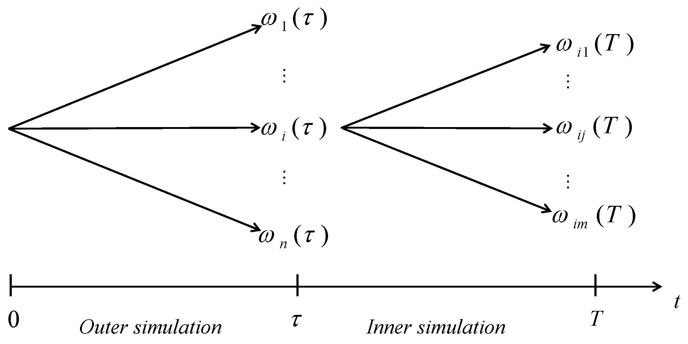
Figure 1. Nested Simulation.
Mathematics 11 01414 g001
Figure 2. The estimated exceedance probability given the estimated VaR in portfolio 1. Set α = 0.95, 0.99 and 0.995. The three subfigures in the first row correspond to α = 0.95 , the three subfigures in the second row correspond to α = 0.99 , and the three subfigures in the third row correspond to α = 0.995 .
Mathematics 11 01414 g002
Figure 3. The estimated exceedance probability given the estimated VaR in portfolio 2. Set α = 0.95, 0.99 and 0.995. The three subfigures in the first row correspond to α = 0.95 , the three subfigures in the second row correspond to α = 0.99 , and the three subfigures in the third row correspond to α = 0.995 .
Mathematics 11 01414 g003
Figure 4. The estimated exceedance probability given the estimated VaR in portfolio 3. Set α = 0.95, 0.99 and 0.995. The three subfigures in the first row correspond to α = 0.95 , the three subfigures in the second row correspond to α = 0.99 , and the three subfigures in the third row correspond to α = 0.995 .
Mathematics 11 01414 g004
Figure 5. The estimated exceedance probability given the estimated VaR in portfolio 4. Set α = 0.95, 0.99 and 0.995. The three subfigures in the first row correspond to α = 0.95 , the three subfigures in the second row correspond to α = 0.99 , and the three subfigures in the third row correspond to α = 0.995 .
Mathematics 11 01414 g005
Table 1. The parameters setting for underlying assets following the Lévy process.
Initial Asset PriceStrike PriceT τ r
Portfolio 1 S 1 = 100 , S 2 = 100 , S 3 = 100 K 1 = 95 , K 2 = 100 , K 3 = 105 10.252%
Portfolio 2 S 1 = 80 , S 2 = 90 , S 3 = 100 K 1 = 80 , K 2 = 90 , K 3 = 100 10.252%
Portfolio 3 S 1 = 100 , S 2 = 100 , S 3 = 100 K 1 = 95 , K 2 = 100 , K 3 = 105 10.252%
Portfolio 4 S 1 = 100 , S 2 = 100 , S 3 = 100 K 1 = 95 , K 2 = 100 , K 3 = 105 10.252%
Table 2. The parameters setting of Lévy process for each underlying asset.
Underlying AssetsLévy ProcessParameters
Asset 1VG σ = 0.2 , ν = 0.3 , θ = 0
Portfolio 1Asset 2VG σ = 0.3 , ν = 0.3 , θ = 0
Asset 3VG σ = 0.4 , ν = 0.3 , θ = 0
Asset 1VG σ = 0.2 , ν = 0.2 , θ = 0.1
Portfolio 2Asset 2VG σ = 0.3 , ν = 0.3 , θ = 0
Asset 3VG σ = 0.4 , ν = 0.4 , θ = 0.1
Asset 1NIG a = 2 , β = 0.2 , γ = 0.8
Portfolio 3Asset 2NIG a = 3 , β = 0.2 , γ = 0.8
Asset 3NIG a = 2 , β = 0.3 , γ = 0.8
Asset 1NIG a = 10 , β = 0.2 , γ = 0.03
Portfolio 4Asset 2NIG a = 11 , β = 0.3 , γ = 0.04
Asset 3NIG a = 12 , β = 0.4 , γ = 0.05
Table 3. rRMSE of estimated VaR in Portfolio 1.
α Basis 1 (%)Basis 2 (%)Basis 3 (%)Basis 4 (%)Basis 5 (%)Basis 6 (%)Basis 7 (%)
0.950.0960.2860.0990.1540.0880.0870.087
0.990.1340.3280.1270.1460.1690.1300.143
0.9950.1630.3020.1570.1630.2120.1600.172
The rRMSE is calculated by Equation (7). The estimation of VaR is replicated 1000 times for each α. Seven basis functions were considered.
Table 4. The rRMSE of estimated VaR in Portfolio 2.
α Basis 1 (%)Basis 2 (%)Basis 3 (%)Basis 4 (%)Basis 5 (%)Basis 6 (%)Basis 7 (%)
0.950.0990.2210.0990.1870.1000.0950.099
0.990.1440.3450.1400.2010.1770.1440.161
0.9950.1710.3480.1690.2040.2180.1740.190
The rRMSE is calculated by Equation (7). The estimation of VaR is replicated 1000 times for each α. Seven basis functions were considered.
Table 5. The rRMSE of estimated VaR in Portfolio 3.
α Basis 1 (%)Basis 2 (%)Basis 3 (%)Basis 4 (%)Basis 5 (%)Basis 6 (%)Basis 7 (%)
0.950.4680.4700.1830.2660.3980.2040.319
0.990.3310.3370.3110.3550.3310.2620.267
0.9950.5000.4100.4020.3820.3920.3820.304
The rRMSE is calculated by Equation (7). The estimation of VaR is replicated 1000 times for each α. Seven basis functions were considered.
Table 6. The rRMSE of estimated VaR in Portfolio 4.
α Basis 1 (%)Basis 2 (%)Basis 3 (%)Basis 4 (%)Basis 5 (%)Basis 6 (%)Basis 7 (%)
0.950.1220.3890.1180.2410.1210.1040.123
0.990.1630.3330.1680.3010.1490.1470.150
0.9950.1900.3950.1920.3110.1820.1710.185
The rRMSE is calculated by Equation (7). The estimation of VaR is replicated 1000 times for each α. Seven basis functions were considered.
Disclaimer/Publisher’s Note: The statements, opinions and data contained in all publications are solely those of the individual author(s) and contributor(s) and not of MDPI and/or the editor(s). MDPI and/or the editor(s) disclaim responsibility for any injury to people or property resulting from any ideas, methods, instructions or products referred to in the content.