MBDM: Multinational Banknote Detecting Model for Assisting Visually Impaired People

Abstract

With the proliferation of smartphones and advancements in deep learning technologies, object recognition using built-in smartphone cameras has become possible. One application of this technology is to assist visually impaired individuals through the banknote detection of multiple national currencies. Previous studies have focused on single-national banknote detection; in contrast, this study addressed the practical need for the detection of banknotes of any nationality. To this end, we propose a multinational banknote detection model (MBDM) and a method for multinational banknote detection based on mosaic data augmentation. The effectiveness of the MBDM is demonstrated through evaluation on a Korean won (KRW) banknote and coin database built using a smartphone camera, a US dollar (USD) and Euro banknote database, and a Jordanian dinar (JOD) database that is an open database. The results show that the MBDM achieves an accuracy of 0.8396, a recall value of 0.9334, and an F1 score of 0.8840, outperforming state-of-the-art methods.

1. Introduction

Smartphones equipped with deep learning technology have the ability to recognize a variety of objects using built-in cameras, including banknotes of multiple nationalities [1,2]. Previous studies on banknote detection have mainly focused on either handcrafted feature-based methods or deep feature-based methods. Handcrafted feature-based methods such as speed up robust features (SURF) have achieved good results in banknote detection [1,2,3,4]. However, deep feature -based methods such as you only look once (YOLO)-v3 have been shown to outperform handcrafted feature-based methods in varied environments, with an F1 score of 0.9184 for YOLO-v3 compared to 0.8139 for SURF [5]. While these existing studies have primarily focused on single-nationality banknote detection, there is a need for a method to detect banknotes of any nationality. However, considering the practicality aspect, banknote input through a camera is required for detection regardless of the type of nationality. In this study, we addressed this problem and devised a multinational banknote detection model (MBDM) and a method for multinational banknote detection based on mosaic data augmentation. The main contributions of this study are as follows:

-

This study is the first on smartphone-based multinational banknote detection.

-

A novel MBDM was developed. The MBDM consists of 69 layers and has a four-step process for feature extraction and final detection. Its feature map configuration is particularly effective at detecting small objects such as coins.

-

The detection performance of the MBDM was improved using mosaic data augmentation to increase training data.

-

The self-constructed Dongguk Multinational Banknote database version 1 (DMB v1) and the MBDM developed in this study were made publicly available on GitHub [6] for fair evaluation by other researchers.

The remainder of this paper is structured as follows. Section 2 reviews the related works of single-national and multinational banknote detection. Section 3 provides a detailed description of the proposed research method of overall procedure, mosaic data augmentation, the architecture of the MBDM, and the mathematical fundamentals of bounding box detection by the MBDM. Section 4 presents the experimental results with Dongguk Korean Banknote database version 1 (DKB v1) [5] including US dollars (USD), Euros (EUR), and Korean won (KRW), and Jordanian dinar (JOD) open database with analysis. Finally, Section 5 summarizes the study and the main findings.

2. Related Works

Existing banknote detection studies can be broadly classified into handcrafted feature-based methods and deep feature-based methods. In handcrafted feature-based methods, techniques such as SURF, fast radial symmetry (FRS) transform, and principal component analysis (PCA) are applied to banknote images for detection and recognition. The SURF method is particularly fast and efficient at localizing and matching banknote features compared to other handcrafted feature-based methods [1,2,3,4]. The SURF method is robust in terms of image rotation or scaling change; however, it may mistakenly recognize the background as a banknote. To address this issue, some studies have used FRS-based banknote recognition by extracting gradients for the numerical part of the banknote [7]. Other handcrafted feature-based methods such as PCA extract denomination types and regions of interest (RoIs) for each denomination type to create eigen-images and then perform banknote recognition based on these eigen-images [8]. There have also been studies that have used the K-nearest neighbors (KNN) classifier [9] or decision tree classifier (DTC) [10] to perform banknote detection on a Malaysian banknote database [11]. However, handcrafted feature-based methods can struggle to maintain good detection or classification performance for banknote data acquired in different environments, leading to the development of deep feature-based methods to overcome these challenges.

Deep convolutional neural networks (DCNNs) have shown better performance in detection and classification compared to handcrafted feature-based methods. There are several types of DCNNs that have been applied to banknote detection including MobileNet, AlexNet, Faster R-CNN, YOLO-v3, and self-designed CNN models. MobileNet [12] is useful for applications with low hardware requirements because it has a small number of parameters and requires minimal computation compared to other compared DCNNs with many layers, for example, GoogleNet or visual geometry group (VGG)-16. However, Faster R-CNN requires high-performance hardware such as a graphics processing unit (GPU) owing to its large number of layers, making it difficult to use on wearable devices with lower performance. As a result, there has been a study that achieved good performance by applying MobileNet to banknote detection on a wearable device [13]. AlexNet [14], which has a structure similar to LeNet and consists of eight layers including five convolution layers and three fully connected layers, can perform training using two GPUs in parallel. There has been a study that used this CNN network for deep feature extraction and then classified banknote objects in images using a support vector machine (SVM) and histogram of oriented gradients (HOG) [15]. Faster R-CNN [16] has also been applied to banknote detection and is known for its excellent detection performance in DCNNs [5]. It obtains feature maps through feature extraction using a CNN such as VGG [17] or a residual network (ResNet) [18] and then uses these feature maps as an input for the region proposal network (RPN) and classifier, which are trained to perform banknote detection. The detection boxes produced by the detection result are filtered for false positives (FPs) through three postprocessing steps. Banknote FPs are removed based on the width-to-height ratio of the detection boxes, and FPs are eliminated if they do not fall within the appropriate range based on the size range of coins and bills. Finally, when there are multiple detection boxes within an image for a single object, only the detection box with the highest score is considered a true positive (TP), and FPs are eliminated to improve detection performance [5]. YOLO-v3 [19,20] has also been applied in some studies. YOLO-v2 [21] used VGG-16 for feature extraction; however, to create a faster model, Darknet-19 was developed and used in YOLO-v2 [21]. YOLO-v3 improves upon YOLO-v2 by using Darknet-53, which has more layers than Darknet-19. The YOLO-v3 method performs better in object detection, particularly for small objects, and is able to achieve real-time detection owing to its improved processing speed. It has been used for banknote detection on India’s banknote dataset and Iraq’s banknote dataset with good speed and performance. In addition, there has been a study on detection and classification using a shallow CNN network with Euro and Mexican banknotes [22], where Euro and Mexican banknotes were trained and tested separately. While these deep feature-based studies have focused on banknotes, there are almost no existing studies on small objects such as coins. While deep feature-based methods have generally shown better detection performance than handcrafted feature-based methods, most existing studies in this field have only focused on single-national banknote detection. There are no existing studies on multinational banknote detection, regardless of the nationality of the banknote. However, it is practical to be able to detect banknotes of any nationality when using a smartphone camera. To address this problem, we propose a method for multinational banknote detection using the MBDM and mosaic data augmentation.

Although they are not related to banknote detection, the authors proposed the method of motion prediction for beating heart surgery with a gated recursive unit (GRU) [23], an improved stereo matching algorithm on the basis of joint similarity measures and adaptive weights [24], reconstructing dynamic soft-tissue using a stereo endoscope on the basis of a single-layer network [25], and endoscope image mosaic on the basis of pyramid oriented fast and rotated brief (ORB) [26]. Table 1 compares the strengths and weaknesses of the previous studies and the proposed method, dividing them into single-nationality banknote databases and multinationality banknote databases.

Table 1. Comparisons of proposed and previous studies on banknote detection.

Category		Methods	Advantages	Disadvantages
Single-national banknote detection	Handcrafted feature-based	SURF-based [1,2,3,4], FRS transform [7], PCA [8], KNN + DTC [11]	- High-performance devices are not required because of the small amount of computation - Applicable to wearable devices or mobile devices	Detection performance is poor in images with complex backgrounds, and limited scale invariance performance
	Deep feature-based	MobileNet [13], AlexNet, SVM, and HOG [15], Faster R-CNN + three step postprocessing [5], YOLO-v3 + data augmentation [19,20], Shallow CNN [22]	- High detection performance in datasets with complex backgrounds - Applicable to wearable devices with the development of shallow deep CNN	Did not perform multinational banknote detection of various nationalities
Multinational banknote detection	Deep feature-based	MBDM (proposed method)	In a multinational banknote environment acquired from various conditions and backgrounds, not only bills but also small-sized coins are detected with high accuracy	Higher computational cost than MobileNet, YOLO-based methods

3. Materials and Methods

3.1. Overall Procedure of Proposed Method

Figure 1 illustrates the overall process of the proposed banknote detection method. The first step is to preprocess the training images to improve the training performance. This is performed using mosaic data augmentation (described in detail in Section 3.2). After preprocessing, the training data are applied to the MBDM for training. When a testing image is input to the trained MBDM, the MBDM outputs the location, type, and classification probability of multinational banknotes.

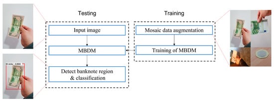
Figure 1. Procedure of proposed method for multinational banknote detection.

3.2. Mosaic Data Augmentation

As shown in Figure 1, the proposed method uses mosaic data augmentation to efficiently train the banknote dataset. Mosaic data augmentation is a type of Bag of Freebies (BoF) data augmentation technique, which was introduced in YOLO-v4 [27] to improve the accuracy of detection by modifying the training method or increasing the training cost of models trained in an offline environment. The advantage of BoF is that it increases the variability of input images and makes the detection model more robust to various images. Because mosaic data augmentation uses banknote data from various nationalities, it is particularly useful for datasets with different classes; it was shown to be effective in this study. As shown in Figure 2a, mosaic data augmentation combines four images from four different classes (dollar, Euro, Korean won, and Jordanian dinar) into one image. The mosaic data augmentation was performed based on the image size of the banknote dataset, and as shown in the right image of Figure 2a, four class images were randomly placed in four zones, with annotations adjusted according to their positions. Four individual annotations are applied to one mosaic data-augmented image, with four class annotations stored in one image. The use of mosaic data augmentation allows for a mini batch size of four. While using mosaic data augmentation, a clear impact of applying the mini batch was observed. In the case of the mosaic data augmentation introduced in YOLO-v4, only four images were introduced. In this study, by contrast, we used a mini batch size of two to compare the effect of using two images and a mini batch size of six to compare the effect of using six, as illustrated in Figure 2b,c.

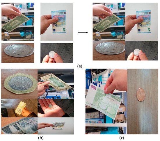
Figure 2. Mosaic data augmentation of banknote dataset: (a) is an example of applying four images of mosaic data augmentation, and (b,c) are examples of applying six images and two images of mosaic data augmentation, respectively.

3.3. Architecture of MBDM

The preprocessed data are fed to the MBDM, a CNN model, for training. The MBDM architecture is based on and improves upon the YOLO-v3 model. It begins with a 3 × 3 (stride = 1) convolution layer and a 3 × 3/2 (stride = 2) convolution layer. It then uses a series of 1 × 1 (stride = 1) convolution, 3 × 3 (stride = 1) convolution, and residual layers, which creates a set, followed by a 3 × 3/2 (stride = 2) convolution layer for downsampling. After the downsampling, the set becomes 8 and convolution is performed. This is repeated 3 times, and at the end of each set, 3 × 3/2 (stride = 2) convolution is applied and downsampling is performed. The eight sets of convolution layers are divided into three parts: the front box set, the middle box set, and the last box set. Training is then completed by applying average pooling, a fully connected layer, and an independent logistic classifier to the output obtained after passing through the set four times. The MBDM consists of a total of 69 convolution layers. Figure 3 provides a visual representation of the structure of the MBDM. The lower part of the figure shows the first prediction proceeding after feature extraction. The green boxed part is the 1 × 1 convolution layer, the yellow boxed part is the upsampling part, and the purple boxed part is the concatenation part. After the first prediction, 1 × 1 convolution is performed and upsampling is performed, followed by concatenation using the features from the front box set. The second prediction is then made, following the same process as the first, with the second concatenation part concatenating with the features of the middle box set. The third prediction is followed by the fourth prediction, which is made by concatenating with the features of the last box set.

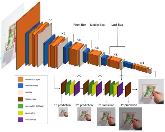
Figure 3. Structure of the MBDM.

Four prediction feature maps are generated in this method, each with dimensions of 13 × 13, 26 × 26, 52 × 52, and 104 × 104 as shown in Figure 4. These feature maps are input into a fully convolutional network (FCN) consisting of 1 × 1 and 3 × 3 convolution layers, and the output channel is increased to 512. The feature map is then upsampled twice and concatenated with the feature map at the next higher resolution. This process is repeated to obtain feature maps at four scales. The number of output channels in the feature map at each scale is determined using a formula that takes into account the anchor box value (3), the bounding box offset value (4), the objectness score (1), and the number of classes. For example, the numbers of 1 × 1 convolution layers for the feature map at each scale would be: box number × (bounding box offset + objectness score + class number) = 3 × (4 + 1 + 26) = 93. The feature maps at each scale will have dimensions of 104 × 104 (×93), 52 × 52 (×93), 26 × 26 (×93), and 13 × 13 (×93). Prediction is performed at larger scales as the feature vector size decreases and at smaller scales as the feature vector size increases. Table 2 shows the detailed structure of the MBDM.

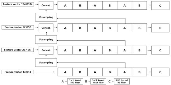
Figure 4. Prediction process. From the bottom to top, the 1st to 4th predictions are presented.

Table 2. Architecture of MBDM.

Layer Number	Number of Iterations	Layer Type	Number of Filters	Filter Size	Output
0		Input_layers	0	0
1		Conv.	32	3 × 3	512 × 512
2		Conv.	64	3 × 3/2	256 × 256
3	×1	Conv.	32	1 × 1
4		Conv.	64	3 × 3
5		Residual			256 × 256
6		Conv.	128	3 × 3/2	128 × 128
7	×2	Conv.	64	1 × 1
8		Conv.	128	3 × 3
9		Residual			128 × 128
10		Conv.	256	3 × 3/2	64 × 64
11	×8	Conv.	128	1 × 1
12		Conv.	256	3 × 3
13		Residual			64 × 64
14		Conv.	512	3 × 3/2	32×32
15	×8	Conv.	256	1 × 1
16		Conv.	512	3 × 3
17		Residual			32 × 32
18		Conv.	1024	3 × 3/2	16 × 16
19	×8	Conv.	512	1 × 1
20		Conv.	1024	3 × 3
21		Residual			16 × 16
22		Conv.	2048	3 × 3/2	8 × 8
23	×4	Conv.	1024	1 × 1
24		Conv.	2048	3 × 3
25		Residual			8 × 8
26		Average pooling	Global
27		Connected	1000
28		Independent logistic classifier

3.4. Mathematical Fundamentals of Bounding Box Detection by MBDM

In training, bounding boxes are defined using $v_x$, $v_y$, $v_w$, and $v_h$ ($v_x$ and $v_y$ represent the x- and y-coordinates of the bounding box in the grid, and $v_w$ and $v_h$ represent the width and height of the bounding box, respectively). The method for determining bounding boxes from YOLO is used and the location coordinates of the bounding box are predicted relative to the grid cell using this method. Further, $t_x,$ $t_y,$ $t_w,\mathrm{a}\mathrm{n}\mathrm{d}$ $t_h$ represent the x- and y-coordinates and the width and height, respectively, and these location coordinates indicate the predicted bounding box. $c_x$ and $c_y$ represent the offset from the top left corner of the grid cell, and $p_w$ and $p_h$ represent the width and height in anchor dimensions. σ() of Equations (1) and (2) is a logistic activation function such as sigmoid function [21]. The bounding box is predicted using $t_x$, $t_y$, $t_w$, $t_h$ and $c_x$, $c_y$ $p_w$, $p_h$, which are calculated using the following formula.

$$v_x=\mathsf{\sigma }(t_x) + c_x$$

(1)

$$v_y=\mathsf{\sigma }(t_y) + c_y$$

(2)

$$v_w=p_w{e}^{t_w}$$

(3)

$$v_h=p_h{e}^{t_h}$$

(4)

4. Experiment Results and Analysis

4.1. Experimental Database and Setup

In this study, we used the Dongguk Korean Banknote database version 1 (DKB v1) [5] and Jordanian dinar (JOD) open database. We also used an integrated multinational banknote database, which included images of USD, EUR, and KRW captured using the Samsung Galaxy Note10 camera [28]. The DKB v1 consists of eight classes of KRW banknotes, including denominations of 10, 50, 100, 500, 1000, 5000, 10,000, and 50,000 as well as coins and bills. It includes a total of 6400 images, with 800 images per class and has a resolution of 1920 × 1080 pixels. The JOD database, which includes both coins and bills, consists of nine classes in denominations of 1 Qirsh 5, 10 Piastres 1/4, 1/2, 1, 5, 1, and 20 Dinars, and has image resolution of 3264 × 2448 pixels. The acquired USD database includes six classes of 1, 5, 10, 20, 50, and 100 dollar bills, with a total of 120 images, 20 images per class, and an image resolution of 1920 × 1080 pixels. The EUR database consists of five classes of 5, 10, 20, 50, and 100 Euro bills, with a total of 100 images (20 images per class) and an image resolution of 1920 × 1080 pixels. However, the input images of all four datasets for the MBDM in Figure 1 are resized to 1024 × 1024 pixels via bilinear interpolation. Therefore, the minimum resolution is 1024 × 1024 pixels to apply our method. Data augmentation was applied to the USD and EUR databases because of their small number of training data. To mimic real-world conditions, the banknote images in all of the databases were acquired at various angles, with folds, and varying contrasts. A detailed description of the experimental databases is provided in Table 3, and examples of database images are presented in Figure 5.

Table 3. Detailed description of database.

Type of Banknote	Denomination	Number of Images	Training	Testing
USD	1 Dollar	660	330	330
	5 Dollar	670	335	335
	10 Dollar	660	330	330
	20 Dollar	670	335	335
	50 Dollar	660	330	330
	100 Dollar	680	340	340
EUR	5 Euro	800	400	400
	10 Euro	800	400	400
	20 Euro	800	400	400
	50 Euro	800	400	400
	100 Euro	800	400	400
KRW	10 Won	800	400	400
	50 Won	800	400	400
	100 Won	800	400	400
	500 Won	800	400	400
	1000 Won	820	410	410
	5000 Won	820	410	410
	10,000 Won	820	410	410
	50,000 Won	820	410	410
JOD	1 piastres	700	350	350
	5 piastres	900	450	450
	10 piastres	240	120	120
	0.25 dinar	580	290	290
	0.5 dinar	480	240	240
	1 dinar	1460	730	730
	5 dinar	580	290	290
	10 dinar	700	350	350
	20 dinar	900	450	450
Total		21,020	10,510	10,510

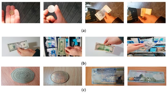
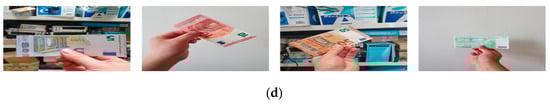
Figure 5. Examples of database images: (a) is KRW, (b) is USD, (c) is JOD, and (d) is EUR.

We trained and tested our algorithm on a desktop computer equipped with Intel^® Core™ i7-950 CPU@3.07GHz, 20 Gigabytes (GB) memory, and NVIDIA GeForce GTX1070 graphics with 1920 compute unified device architecture (CUDA) cores [29]. The algorithm was implemented using PyTorch [30] in Python [31] and utilized CUDA (Version 10.0) [32] with CUDA deep neural network library (CUDNN) (version 7.1.4) [33].

4.2. Training of Proposed Method

For this study, as described in Table 3, a total of 21,020 images were divided into training and testing sets of 10,510 images, and two-fold cross-validation was performed.

This implies that in the first fold, 10,510 images were used for training and the remaining 10,510 images were used for testing. In the second fold, these two sets were exchanged for training and testing. The final performance was determined by taking average accuracy across the two-fold experiments. In addition, we selected 1000 images of each nationality from the training set to use as a validation dataset, totaling 4000 images. The parameters used for training in this study included a base learning rate of 0.001, batch size of 1, gamma of 0.1, weight decay of 0.0005, and 150 epochs. An adaptive moment estimation (Adam) optimizer was also used. Figure 6a,b show training loss and accuracy, as well as the validation loss and accuracy, for the first and second folds of the MBDM, respectively. As shown in these figures, the training loss and accuracy values converge as the number of epochs increases, indicating that the MBDM has been adequately trained on the training data. In addition, the convergence of the validation loss and accuracy values as the number of epochs increases suggests that the MBDM is not overfitted to the training data.

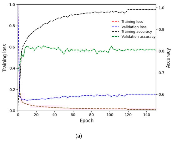
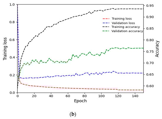
Figure 6. Training and validation loss and accuracy graphs of MBDM: (a) is the loss and accuracy for the training and validation data in the first fold, and (b) is the loss and accuracy for the training and validation data in the second fold.

4.3. Testing of Proposed Method

4.3.1. Evaluation Metric

To measure the testing performance, we calculated true positive (TP), false positive (FP), and false negative (FN) values based on the intersection over union (IoU) value between the detection box and the ground-truth box obtained through the proposed MBDM. We then used the obtained TP, FP, and FN values to calculate precision, recall, and F1 score using the equations below, and evaluated the testing performance accordingly. In Equations (5)–(7), #TP, #FP, and #FN represent the number of TP, FP, and FN, respectively [34].

$$\mathrm{P}\mathrm{r}\mathrm{e}\mathrm{c}\mathrm{i}\mathrm{s}\mathrm{i}\mathrm{o}\mathrm{n}=\frac{\#\mathrm{T}\mathrm{P}}{\#\mathrm{T}\mathrm{P}+\#\mathrm{F}\mathrm{P}}$$

(5)

$$\mathrm{R}\mathrm{e}\mathrm{c}\mathrm{a}\mathrm{l}\mathrm{l}=\frac{\#\mathrm{T}\mathrm{P}}{\#\mathrm{T}\mathrm{P}+\#\mathrm{F}\mathrm{N}}$$

(6)

$$\mathrm{F}1 \mathrm{s}\mathrm{c}\mathrm{o}\mathrm{r}\mathrm{e}=\frac{2·\mathrm{p}\mathrm{r}\mathrm{e}\mathrm{c}\mathrm{i}\mathrm{s}\mathrm{i}\mathrm{o}\mathrm{n}·\mathrm{r}\mathrm{e}\mathrm{c}\mathrm{a}\mathrm{l}\mathrm{l}}{\mathrm{p}\mathrm{r}\mathrm{e}\mathrm{c}\mathrm{i}\mathrm{s}\mathrm{i}\mathrm{o}\mathrm{n}+\mathrm{r}\mathrm{e}\mathrm{c}\mathrm{a}\mathrm{l}\mathrm{l}}$$

(7)

4.3.2. Ablation Studies

We conducted ablation studies to compare three methods. The first method involved using Retinex filtering [35] before applying the MBDM to the input image, while the second method involved using grouped convolution [36] in the MBDM. The third method involved using mosaic data argumentation for MBDM training. As shown in Table 4, both precision and recall performances were lower when Retinex filtering was applied compared to when it was not applied. Grouped convolution was applied to improve the speed and performance of the operation; however, Table 5 shows that performance was higher when it was not used. Table 6 shows that mosaic augmentation with four images resulted in higher accuracy compared to two or six images and also showed higher accuracy compared to the case with no mosaic augmentation. Although the authors showed that applying four images in the existing method [27] was effective for mosaic augmentation, they did not perform the ablation studies to select the optimal number of mosaic images. Furthermore, they used ImageNet (ILSVRC 2012 val) and MS COCO (test-dev 2017) datasets, which have different image characteristics from our experimental datasets of USD, EUR, KRW, and JOD banknotes. Therefore, we performed the ablation studies to select the optimal number of mosaic images as shown in Table 6 and found that four images for mosaic augmentation has the highest accuracies.

Table 4. Performance comparisons with or without Retinex filtering.

Method	Precision	Recall	F1 Score
With Retinex	0.8053	0.8737	0.8381
Without Retinex (proposed method)	0.8396	0.9334	0.8840

Table 5. Performance comparisons with or without grouped convolution.

Method	Precision	Recall	F1 Score
With grouped convolution	0.8294	0.9255	0.8748
Without grouped convolution (proposed method)	0.8396	0.9334	0.8840

Table 6. Performance comparisons with or without mosaic augmentation, and with mosaic augmentation according to the various number of images.

Method		Precision	Recall	F1 Score
Without mosaic augmentation		0.8242	0.9263	0.8723
With mosaic augmentation using	two images	0.8173	0.9097	0.8610
	four images	0.8396	0.9334	0.8840
	six images	0.8166	0.8885	0.8510

As shown in Figure 3 and Table 2, the proposed MBDM consists of three box sets. We added one more box set with the same configuration to create the MBDM (deeper layers), resulting in a model with deeper layers (85 layers). We compared the performance of the MBDM (normal layers) and the MBDM (deeper layers) in Table 7. When mosaic augmentation is not used, the MBDM (deeper layers) exhibited lower precision performance but higher recall performance compared to the MBDM (normal layers). However, in terms of final F1 score, the MBDM (deeper layers) performed better. When we applied the same mosaic augmentation with four images, the MBDM (normal layers) showed higher accuracy, and the MBDM (normal layers) with mosaic augmentation using four images showed the highest performance in all cases.

Table 7. Performance comparisons according to MBDM (normal layers) and MBDM (deeper layers) with or without mosaic augmentation.

Method		Precision	Recall	F1 Score
Without mosaic augmentation	MBDM (deeper layers)	0.8150	0.9424	0.8741
	MBDM (normal layers)	0.8242	0.9263	0.8723
With mosaic augmentation (four images)	MBDM (deeper layers)	0.8359	0.9255	0.8784
	MBDM (normal layers)	0.8396	0.9334	0.8840

4.3.3. Comparisons with the State-of-the-Art Methods

In this subsection, we compare the performance of the proposed method with state-of-the-art methods. We compared our method with deep feature-based methods such as the MobileNet-based banknote detection method [13], the Faster R-CNN-based banknote detection method [5], the YOLO v3-based banknote detection method [19,20], and the YOLO v2 [21] method. As shown in Table 8, the proposed method outperformed the state-of-the-art methods in the multinational banknote database. MobileNet [13] exhibited the worst performance, while Faster R-CNN performed better than YOLO v2. In terms of precision, Faster R-CNN achieved a slightly higher score than YOLO v3; however, in terms of recall, YOLO v3 performed better. In terms of the final performance metric, the F1 score, YOLO v3 exhibited the highest results. Table 9 and Table 10 compare the performance of the state-of-the-art methods and the proposed method for USD and EUR. As described in Section 4.1, the USD and EUR databases contain only bills; therefore, we only compare the detection accuracy for bills. As shown in Table 9 and Table 10, the proposed method showed higher performance than the state-of-the-art methods. Finally, Table 11 and Table 12 compare the performance of the state-of-the art methods and the proposed method for KRW and JOD. As described in Section 4.1, the KRW and JOD database contain both coins and bills, so we compare the detection accuracy of coins and bills, respectively. As shown in Table 11 and Table 12, the proposed method showed higher performance than the state-of-the-art methods. Upon comparing Table 9 and Table 10 with Table 11 and Table 12, it is evident that the accuracy of the proposed method is relatively higher in the USD and EUR databases than in the KRW and JOD databases. This is because the KRW and JOD databases contain coin data, which have a smaller size and more light reflection on the metal surface, leading to lower detection accuracy compared to bills, which have a larger size and relatively less light reflection. Figure 7, Figure 8, Figure 9, Figure 10 and Figure 11 compare the results of Table 8, Table 9, Table 10, Table 11 and Table 12 according to the IoU threshold; evidently, the proposed method showed higher detection accuracy than the state-of-the-art methods.

Table 8. Performance comparisons of the proposed method and the state-of-the-art methods with multinational banknote database.

Methods		Precision	Recall	F1 Score
Faster R-CNN [5]	Coin	0.7576	0.8210	0.7880
	Bill	0.8410	0.9114	0.8748
	Coin and bill	0.7993	0.8662	0.8314
YOLO v3 [19,20]	Coin	0.7351	0.8272	0.7783
	Bill	0.8629	0.9710	0.9137
	Coin and bill	0.7990	0.8991	0.8460
MobileNet [13]	Coin	0.7472	0.7911	0.7685
	Bill	0.8376	0.8867	0.8614
	Coin and bill	0.7924	0.8389	0.8150
YOLO v2 [21]	Coin	0.7371	0.7906	0.7630
	Bill	0.8653	0.9282	0.8956
	Coin and bill	0.8012	0.8594	0.8293
YOLO v4 [27]	Coin	0.7763	0.8657	0.8186
	Bill	0.8713	0.9715	0.9187
	Coin and bill	0.8238	0.9186	0.8686
YOLO v5 [37]	Coin	0.7771	0.8608	0.8168
	Bill	0.8731	0.9672	0.9178
	Coin and bill	0.8251	0.914	0.8673
MBDM (proposed method)	Coin	0.7747	0.8707	0.8200
	Bill	0.8737	0.9819	0.9246
	Coin and bill	0.8396	0.9334	0.8840

Table 9. Performance comparisons of the proposed method and the state-of-the-art methods with USD.

Methods	Precision	Recall	F1 Score
Faster R-CNN [5]	0.8465	0.9173	0.8805
YOLO v3 [19,20]	0.8752	0.9848	0.9268
MobileNet [13]	0.8196	0.8676	0.8429
YOLO v2 [21]	0.8752	0.9388	0.9059
YOLO v4 [27]	0.8804	0.9745	0.9251
YOLO v5 [37]	0.8795	0.9815	0.9277
MBDM (proposed method)	0.8861	0.9957	0.9377

Table 10. Performance comparisons of the proposed method and the state-of-the-art methods with EUR.

Methods	Precision	Recall	F1 Score
Faster R-CNN [5]	0.8472	0.9181	0.8812
YOLO v3 [19,20]	0.8739	0.9834	0.9254
MobileNet [13]	0.8486	0.8983	0.8727
YOLO v2 [21]	0.8747	0.9383	0.9054
YOLO v4 [27]	0.8756	0.9839	0.9266
YOLO v5 [37]	0.8841	0.9785	0.9289
MBDM (proposed method)	0.8855	0.9952	0.9372

Table 11. Performance comparisons of the proposed method and the state-of-the-art methods with KRW.

Methods		Precision	Recall	F1 Score
Faster R-CNN [5]	Coin	0.7600	0.8236	0.7905
	Bill	0.8356	0.9055	0.8691
	Coin and bill	0.7978	0.8646	0.8298
YOLO v3 [19,20]	Coin	0.7258	0.8167	0.7686
	Bill	0.8520	0.9587	0.9022
	Coin and bill	0.7889	0.8877	0.8354
MobileNet [13]	Coin	0.7392	0.7826	0.7603
	Bill	0.8286	0.8772	0.8522
	Coin and bill	0.7839	0.8299	0.8062
YOLO v2 [21]	Coin	0.7262	0.7789	0.7516
	Bill	0.8524	0.9143	0.8823
	Coin and bill	0.7893	0.8466	0.8169
YOLO v4 [27]	Coin	0.7573	0.8632	0.8068
	Bill	0.8489	0.9676	0.9043
	Coin and bill	0.8031	0.9154	0.8556
YOLO v5 [37]	Coin	0.7625	0.8496	0.8037
	Bill	0.8563	0.9542	0.9026
	Coin and bill	0.8094	0.9019	0.8532
MBDM (proposed method)	Coin	0.7681	0.8632	0.8129
	Bill	0.8661	0.9734	0.9166
	Coin and bill	0.8171	0.9183	0.8647

Table 12. Performance comparisons of the proposed method and the state-of-the-art methods with JOD.

Methods		Precision	Recall	F1 Score
Faster R-CNN [5]	Coin	0.7552	0.8184	0.7855
	Bill	0.8349	0.9048	0.8684
	Coin and bill	0.7951	0.8616	0.8270
YOLO v3 [19,20]	Coin	0.7228	0.8134	0.7654
	Bill	0.8485	0.9548	0.8985
	Coin and bill	0.7857	0.8841	0.8320
MobileNet [13]	Coin	0.7334	0.7765	0.7543
	Bill	0.8221	0.8703	0.8455
	Coin and bill	0.7777	0.8234	0.7999
YOLO v2 [21]	Coin	0.7334	0.7765	0.7543
	Bill	0.8491	0.9108	0.8789
	Coin and bill	0.7862	0.8433	0.8138
YOLO v4 [27]	Coin	0.7496	0.8405	0.7925
	Bill	0.8410	0.9429	0.8890
	Coin and bill	0.7953	0.8917	0.8407
YOLO v5 [37]	Coin	0.7274	0.8425	0.7807
	Bill	0.8150	0.9439	0.8747
	Coin and bill	0.7712	0.8932	0.8277
MBDM (proposed method)	Coin	0.7651	0.8598	0.8097
	Bill	0.8627	0.9696	0.9131
	Coin and bill	0.8139	0.9147	0.8614

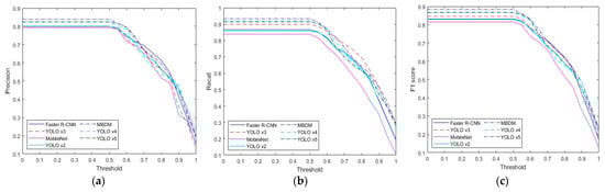
Figure 7. Performance comparison graph for each method according to IoU threshold in multinational banknote database: (a) precision, (b) recall, and (c) F1 score.

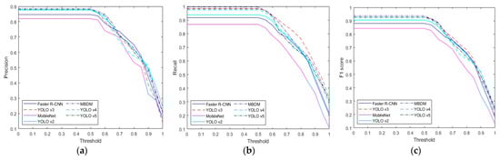
Figure 8. Performance comparison graph for each method according to IoU threshold in USD database: (a) precision, (b) recall, and (c) F1 score.

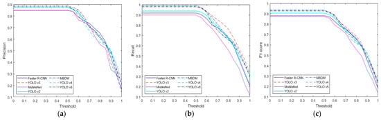
Figure 9. Performance comparison graph for each method according to IoU threshold in EUR database: (a) precision, (b) recall, and (c) F1 score.

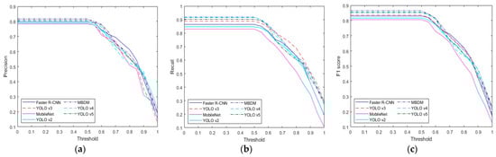
Figure 10. Performance comparison graph for each method according to IoU threshold in KRW database: (a) precision, (b) recall, and (c) F1 score.

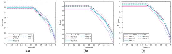
Figure 11. Performance comparison graph for each method according to IoU threshold in JOD database: (a) precision, (b) recall, and (c) F1 score.

4.3.4. Analysis

We compared the experimental results of this study to demonstrate successful detections and cases wherein detection errors occurred. As shown in Figure 12, out of the six detection results, the three examples corresponding to Figure 12a are USD 5, EUR 10, and EUR 100, which represent successful object detection and classification. In particular, Figure 12a shows that these bills were properly detected despite the complex backgrounds, various sizes, and in-plane rotation. The three examples corresponding to Figure 12b are KRW 50, USD 50, and JOD 10, which are cases where a detection error occurred. In the case of KRW 50, the coin is smaller than other banknote objects, and especially smaller than other coins, so it was incorrectly detected as a different coin class during the detection process. In the case of USD 50, a detection error occurred because of the complicated background, whereas in the case of JOD 10, a detection error occurred owing to the folded state of the bill.

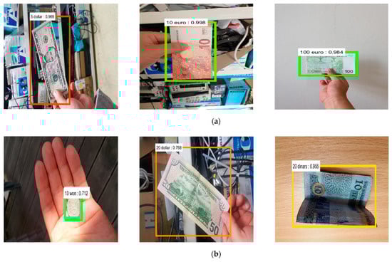
Figure 12. The detection results of the proposed method: (a) is the case where the detection was successful, and (b) is the case where the detection error occurred.

In the next experiment, we extracted the gradient class activation map (GradCAM) [38] from each layer of the proposed MBDM, and the results are shown in Figure 13. GradCAM images can visually indicate the importance of extracted features by displaying important features in a color close to red and unimportant features in a color close to blue in the extracted feature map [38]. We obtained GradCAM from conv_8, conv_12, conv_16, conv_20, and conv_24 of the feature extractor in Table 2, using a JOD 20 bill, KRW 1000 bill, JOD 5 coin, and EUR 100 bill as input. As shown in Figure 13, it was confirmed that highly activated important features are well detected in the banknote and coin regions in the feature map obtained from conv_24 of the MBDM. This confirms that the proposed MBDM extracts important features that can effectively detect banknotes.

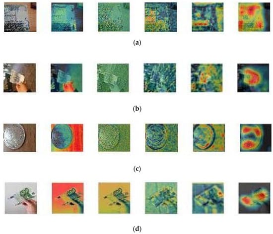
Figure 13. Examples of GradCAM images from MBDM, (a–d) are with the inputs of JOD 20 dinar, KRW 1000 bill, JOD 5 dinar coin, and EUR 100 bill, respectively. GradCAM images extracted from input, conv_8, conv_12, conv_16, conv_20, conv_24 of Table 2 from the left of (a–d).

In the next experiment, we performed a t-test [39] and measured Cohen’s d-value [40] between F1 scores for the proposed MBDM and the second-best method in Table 8 for statistical testing. These tests were conducted for the F1 scores of the coin, bill, and coin and bill databases, respectively. A Cohen’s d-value around 0.2 represents a small effect size, 0.5 means a medium effect size, and 0.8 means a large effect size. As shown in Figure 14a, we measured the p-values of the second-best method and the proposed method for the coin database in Table 8. The p-value of the result was 0.022, which implies a 95% confidence level, and Cohen’s d-value was 4.858 (large effect size). As shown in Figure 14b, we measured the p-values of the second-best method and the proposed method for the bill database in Table 8. The p-value of the result was 0.017, which means a 95% confidence level, and Cohen’s d-value was 5.295 (large effect size). As shown in Figure 14c, we measured the p-values of the second-best method and the proposed method for the coin and bill database in Table 8. The p-value of the result was 0.019, which means a 95% confidence level, and Cohen’s d-value was 5.031 (large effect size). These results confirm that there is a significant difference between the F1 scores of the proposed method and the second-best method in Table 8.

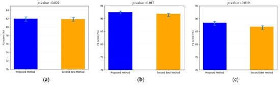
Figure 14. The t-test results between F1 scores of the proposed method and the second-best method in case of (a) coin database, (b) bill database, and (c) coin and bill database.

4.3.5. Comparisons of Inference Time and Model Complexity

This subsection compares the inference time, processing speed, number of model parameters, GPU memory requirements, and the number of floating-point operations per second (#FLOPs) of the proposed method (MBDM) with state-of-the-art methods. The performance metrics were measured on both a desktop computer (described in Section 4.1) and a Jetson TX2 embedded system (shown in Figure 15). Jetson TX2 uses a NVIDIA PascalTM-family GPU and has 256 CUDA cores, 8 GB of memory shared between the central processing unit (CPU) and GPU, and 59.7 GB/s of memory bandwidth, and a power consumption of less than 7.5 W [41]. The MBDM was tested for inference time and processing speed on both a desktop computer and the Jetson TX2 embedded system. The results, shown in Table 13, indicate that the inference time per image was 11.32 ms on the desktop computer and 57.32 ms on the Jetson TX2. This translates to a processing speed of 88.34 frames per second (fps) (1000/11.32) on the desktop computer and 17.45 fps (1000/57.32) on the Jetson TX2. These results demonstrate that the proposed method can be operated on both desktop computers and embedded systems with limited computing resources. However, as shown in Table 13, the MBDM has a slower processing speed than other models but a faster processing speed than Faster R-CNN. In terms of model parameters, GPU memory requirements, and the number of floating-point operations per second (#FLOPs), as shown in Table 14, the MBDM has more parameters than other models and requires less GPU memory than Faster R-CNN and YOLO v4. In addition, it requires less FLOPs than Faster R-CNN. Nevertheless, the proposed method exhibits higher detection accuracy than other methods, as shown in Table 8, Table 9, Table 10, Table 11 and Table 12 and Figure 7, Figure 8, Figure 9, Figure 10 and Figure 11.

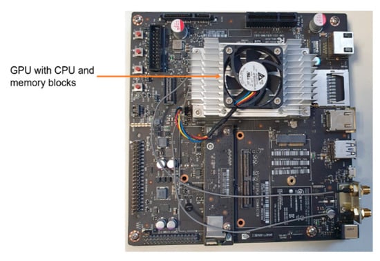
Figure 15. Jetson TX2 embedded system.

Table 13. Comparisons of inference time and processing speed by proposed method and the state-of-the-art methods.

Environment		Inference Time per One Image (Unit: ms)	Processing Speed (Unit: frames/s)
Desktop	Faster R-CNN [5]	12.52	79.87
	YOLO v3 [19,20]	9.81	101.94
	MobileNet [13]	7.59	131.75
	YOLO v2 [21]	10.38	96.34
	YOLO v4 [27]	10.11	98.91
	YOLO v5 [37]	9.96	100.4
	MBDM (proposed method)	11.32	88.34
Jetson embedded system	Faster R-CNN [5]	63.25	15.81
	YOLO v3 [19,20]	48.79	20.50
	MobileNet [13]	31.62	31.63
	YOLO v2 [21]	51.45	19.44
	YOLO v4 [27]	49.82	20.07
	YOLO v5 [37]	48.88	20.46
	MBDM (proposed method)	57.32	17.45

Table 14. Comparisons of number of parameters, GPU memory requirement, and #FLOPs.

Method	# Parameters $\mathbf{(}\mathbf{\times }{\mathbf{10}}^{\mathbf{6}}\mathbf{)}$	GPU Memory Requirement (Unit: Gbyte)	#FLOPs $\mathbf{(}\mathbf{\times }{\mathbf{10}}^{\mathrm{9}}\mathbf{)}$
Faster R-CNN [5]	65.2563	4.138	2.1592
YOLO v3 [19,20]	63.3524	2.285	1.7420
MobileNet [13]	13.1526	1.159	0.7492
YOLO v2 [21]	53.0006	2.293	1.6549
YOLO v4 [27]	64.1748	2.315	1.7951
YOLO v5 [37]	56.1049	1.951	1.5832
MBDM (proposed method)	68.2594	2.312	1.8472

5. Conclusions

In this study, a novel method for detecting banknotes using smartphone images taken under various conditions with various banknote types and complex backgrounds was developed. The proposed method, called the MBDM, was trained using mosaic data augmentation and tested on several databases including DKB v1, a KRW database built for this research, a JOD database (open database), and a multinational banknote database comprising USD and EUR images captured with a Samsung Galaxy Note 10 camera. The results showed that the MBDM outperformed state-of-the-art methods in terms of detection accuracy. The visualization of GradCAM images confirmed that the MBDM adequately extracted important features for accurate detection. Statistical analysis using t-test and Cohen’s d-value also revealed that the proposed method exhibited significantly higher accuracy than the second-best method.

We consider that the execution of our algorithm, database storage, and model training can be performed via cloud computing. However, we also consider a scenario where our algorithm works on an embedded system in a mobile phone. Therefore, we compared the inference time and processing speed of our proposed method and the state-of-the-art methods on a desktop computer and a Jetson embedded system as shown in Table 13, and compared the number of parameters, GPU memory requirement, and #FLOPs as shown in Table 14. These results show that our algorithm can work on an embedded system with limited computing power and memory. However, the detection performance was not always satisfactory, especially for small coins such as KRW 50 or in the case of complicated backgrounds or folded banknotes.

To address these issues, future research will focus on methods for maintaining spatial features to improve detection performance for small objects and for handling complicated backgrounds and folded banknotes. In addition, efforts will be made to reduce the processing time, number of parameters, memory usage, and #FLOPs of the MBDM while maintaining its accuracy.

References

- Sanchez, G.A.R. A computer vision-based banknote recognition system for the blind with an accuracy of 98% on smartphone videos. J. Korea Soc. Comput. Inform. 2019, 24, 67–72. [Google Scholar]
- Sanchez, G.A.R.; Uh, Y.J.; Lim, K.; Byun, H. Fast banknote recognition for the blind on real-life mobile videos. In Proceedings of the Korean Society of Computer Information Conference, Jeju Island, Republic of Korea, 24–26 June 2015; pp. 835–837. [Google Scholar]
- Hasanuzzaman, F.M.; Yang, X.; Tian, Y. Robust and effective component-based banknote recognition by SURF features. In Proceedings of the 2011 20th Annual Wireless and Optical Communications Conference (WOCC), Newark, NJ, USA, 15–16 April 2011; pp. 1–6. [Google Scholar]
- Dunai, L.D.; Pérez, M.C.; Peris-Fajarnés, G.; Lengua, I.L. Euro Banknote Recognition System for Blind People. Sensors 2017, 17, 184. [Google Scholar] [CrossRef]
- Park, C.; Cho, S.W.; Baek, N.R.; Choi, J.; Park, K.R. Deep Feature-Based Three-Stage Detection of Banknotes and Coins for Assisting Visually Impaired People. IEEE Access 2020, 8, 184598–184613. [Google Scholar] [CrossRef]
- MBDM with Algorithms. Available online: https://github.com/channygrad/MBDM/tree/main/MBDM (accessed on 3 March 2023).
- Domínguez, A.R.; Alvarez, C.L.; Corrochano, E.B. Automated banknote identification method for the visually impaired. In Progress in Pattern Recognition, Image Analysis, Computer Vision, and Applications, Proceedings of the 19th Iberoamerican Congress, CIARP 2014, Puerto Vallarta, Mexico, 2–5 November 2014; Springer: Cham, Switzerland, 2014; pp. 572–579. [Google Scholar]
- Grijalva, F.; Rodriguez, J.C.; Larco, J.; Orozco, L. Smartphone recognition of the U.S. banknotes’ denomination, for visually impaired people. In Proceedings of the 2010 IEEE ANDESCON, Bogota, Colombia, 15–17 September 2010; pp. 1–6. [Google Scholar]
- Cunningham, P.; Delany, S.J. K-nearest neighbour classifiers. arXiv 2020, arXiv:2004.04523. [Google Scholar]
- Swain, P.H.; Hauska, H. The decision tree classifier: Design and potential. IEEE Trans. Geosci. Electron. 1977, 15, 142–147. [Google Scholar] [CrossRef]
- Sufri, N.A.J.; Rahmad, N.A.; As’ari, M.A.; Zakaria, N.A.; Jamaludin, M.N.; Ismail, L.H.; Mahmood, N.H. Image based ringgit banknote recognition for visually impaired. J. Telecomm. Electronic Comput. Eng. 2017, 9, 103–111. [Google Scholar]
- Howard, A.G.; Zhu, M.; Chen, B.; Kalenichenko, D.; Wang, W.; Weyand, T.; Andreetto, M.; Adam, H. MobileNets: Efficient Convolutional Neural Networks for Mobile Vision Applications. arXiv 2017, arXiv:1704.04861. [Google Scholar]
- Mittal, S.; Mittal, S. Indian banknote recognition using convolutional neural network. In Proceedings of the 2018 3rd International Conference On Internet of Things: Smart Innovation and Usages (IoT-SIU), Bhimtal, India, 23–24 February 2018. [Google Scholar]
- Krizhevsky, A.; Sutskever, I.; Hinton, G.E. Imagenet classification with deep convolutional networks. In Proceedings of the 26th Annual Conference on Neural Information Processing Systems (NIPS), Lake Tahoe, NV, USA, 3–6 December 2012; pp. 1106–1114. [Google Scholar]
- Imad, M.; Ullah, F.; Hassan, M.A.; Naimullah, M.A. Pakistani Currency Recognition to Assist Blind Person Based on Convolutional Neural Network. J. Comput. Sci. Technol. Stud. 2020, 2, 12–19. [Google Scholar]
- Ren, S.; He, K.; Girshick, R.; Sun, J. Faster R-CNN: Towards real-time object detection with region proposal networks. IEEE Trans. Pattern Anal. Mach. Intell. 2017, 39, 1137–1149. [Google Scholar] [CrossRef] [PubMed]
- Simonyan, K.; Zisserman, A. Very deep convolutional networks for large-scale image recognition. In Proceedings of the International Conference on Learning Representations, San Diego, CA, USA, 7–9 May 2015; pp. 1–14. [Google Scholar]
- He, K.; Zhang, X.; Ren, S.; Sun, J. Deep residual learning for image recognition. In Proceedings of the IEEE Conference on Computer Vision and Pattern Recognition (CVPR), Las Vegas, NV, USA, 26 June–1 July 2016; pp. 770–778. [Google Scholar]
- Joshi, R.C.; Yadav, S.; Dutta, M.K. YOLO-v3 Based Currency Detection and Recognition System for Visually Impaired Persons. In Proceedings of the 2020 International Conference on Contemporary Computing and Applications (IC3A), Lucknow, India, 5–7 February 2020; pp. 280–285. [Google Scholar]
- Mahmood, R.R.; Younus, M.D.; Khalaf, E.A. Currency Detection for Visually Impaired Iraqi Banknote as a Study Case. Turkish J. Comput. Math. Educ. 2021, 12, 2940–2948. [Google Scholar]
- Redmon, J.; Farhadi, A. YOLO9000: Better, faster, stronger. arXiv 2016, arXiv:1612.08242. [Google Scholar]
- Pérez, D.G.; Corrochano, E.B. Recognition system for Euro and Mexican banknotes based on deep learning with real scene images. Comput. Sist. 2018, 22, 1065–1076. [Google Scholar]
- Yang, B.; Li, Y.; Zheng, W.; Yin, Z.; Liu, M.; Yin, L.; Liu, C. Motion prediction for beating heart surgery with GRU. Biomed. Signal Process. Control 2023, 83, 104641. [Google Scholar] [CrossRef]
- Lai, X.; Yang, B.; Ma, B.; Liu, M.; Yin, Z.; Yin, L.; Zheng, W. An improved stereo matching algorithm based on joint similarity measure and adaptive weights. Appl. Sci. 2022, 13, 514. [Google Scholar] [CrossRef]
- Yang, B.; Xu, S.; Chen, H.; Zheng, W.; Liu, C. Reconstruct dynamic soft-tissue with stereo endoscope based on a single-layer network. IEEE Trans. Image Process. 2022, 31, 5828–5840. [Google Scholar] [CrossRef] [PubMed]
- Zhang, Z.; Wang, L.; Zheng, W.; Yin, L.; Hu, R.; Yang, B. Endoscope image mosaic based on pyramid ORB. Biomed. Signal Process. Control 2022, 71 Pt B, 103261. [Google Scholar] [CrossRef]
- Bochkovskiy, A.; Wang, C.; Liao, H.M. Yolov4: Optimal speed and accuracy of object detection. arXiv 2020, arXiv:2004.10934. [Google Scholar]
- Samsung Galaxy Note 10. Available online: https://en.wikipedia.org/wiki/Samsung_Galaxy_Note_10 (accessed on 19 December 2022).
- NVIDIA GeForce GTX 1070. Available online: https://www.nvidia.com/en-in/geforce/products/10series/geforce-gtx-1070/ (accessed on 26 March 2022).
- Pytorch. Available online: https://pytorch.org/docs/stable/index.html (accessed on 26 March 2022).
- Python. Available online: https://docs.python.org/3.7/whatsnew/changelog.html#python-3-7-0-alpha-1 (accessed on 26 March 2022).
- CUDA. Available online: https://en.wikipedia.org/wiki/CUDA (accessed on 26 March 2022).
- CUDNN. Available online: https://developer.nvidia.com/cudnn (accessed on 26 March 2022).
- Precision and Recall. Available online: https://en.wikipedia.org/wiki/Precision_and_recall (accessed on 29 January 2022).
- Parihar, A.S.; Singh, S. A study on Retinex based method for image enhancement. In Proceedings of the 2018 2nd International Conference on Inventive Systems and Control (ICISC), Coimbatore, India, 19–20 January 2018; pp. 619–624. [Google Scholar]
- Krizhevsky, A.; Sutskever, I.; Hinton, G.E. ImageNet classification with deep convolutional neural networks. Commun. ACM 2017, 60, 84–90. [Google Scholar] [CrossRef]
- YOLO v5. Available online: https://pytorch.org/hub/ultralytics_yolov5/ (accessed on 28 February 2023).
- Selvaraju, R.R.; Cogswell, M.; Das, A.; Vedantam, R.; Parikh, D.; Batra, D. Grad-cam: Visual explanations from deep networks via gradient-based localization. In Proceedings of the IEEE International Conference on Computer Vision (ICCV), Venice, Italy, 22–29 October 2017; pp. 618–626. [Google Scholar]
- Student’s T-Test. Available online: https://en.wikipedia.org/wiki/Student%27s_t-test (accessed on 27 December 2020).
- Cohen, J. A power primer. Psychol. Bull. 1992, 112, 155. [Google Scholar] [CrossRef]
- Jetson TX2 Module. Available online: https://developer.nvidia.com/embedded/jetson-tx2 (accessed on 22 April 2022).
Disclaimer/Publisher’s Note: The statements, opinions and data contained in all publications are solely those of the individual author(s) and contributor(s) and not of MDPI and/or the editor(s). MDPI and/or the editor(s) disclaim responsibility for any injury to people or property resulting from any ideas, methods, instructions or products referred to in the content. |
© 2023 by the authors. Licensee MDPI, Basel, Switzerland. This article is an open access article distributed under the terms and conditions of the Creative Commons Attribution (CC BY) license (https://creativecommons.org/licenses/by/4.0/).