Computational Analysis of Hemodynamic Indices Based on Personalized Identification of Aortic Pulse Wave Velocity by a Neural Network

Abstract

Adequate personalized numerical simulation of hemodynamic indices in coronary arteries requires accurate identification of the key parameters. Elastic properties of coronary vessels produce a significant effect on the accuracy of simulations. Direct measurements of the elasticity of coronary vessels are not available in the general clinic. Pulse wave velocity (AoPWV) in the aorta correlates with aortic and coronary elasticity. In this work, we present a neural network approach for estimating AoPWV. Because of the limited number of clinical cases, we used a synthetic AoPWV database of virtual subjects to train the network. We use an additional set of AoPWV data collected from real patients to test the developed algorithm. The developed neural network predicts brachial–ankle AoPWV with a root-mean-square error (RMSE) of $1.3$ m/s and a percentage error of $16\%$. We demonstrate the relevance of a new technique by comparing invasively measured fractional flow reserve (FFR) with simulated values using the patient data with constant ($7.5$ m/s) and predicted AoPWV. We conclude that patient-specific identification of AoPWV via the developed neural network improves the estimation of FFR from $4.4\%$ to $3.8\%$ on average, with a maximum difference of $2.8\%$ in a particular case. Furthermore, we also numerically investigate the sensitivity of the most useful hemodynamic indices, including FFR, coronary flow reserve (CFR) and instantaneous wave-free ratio (iFR) to AoPWV using the patient-specific data. We observe a substantial variability of all considered indices for AoPWV below 10 m/s and weak variation of AoPWV above 15 m/s. We conclude that the hemodynamic significance of coronary stenosis is higher for the patients with AoPWV in the range from 10 to 15 m/s. The advantages of our approach are the use of a limited set of easily measured input parameters (age, stroke volume, heart rate, systolic, diastolic and mean arterial pressures) and the usage of a model-generated (synthetic) dataset to train and test machine learning methods for predicting hemodynamic indices. The application of our approach in clinical practice saves time, workforce and funds.

1. Introduction

Coronary artery disease (CAD) is one of the leading reasons for disability or death in the world. Stenosis of the coronary artery is a common reason for CAD. The hemodynamic significance of stenosis dictates a choice between noninvasive treatment (e.g., drug administration) and surgical procedures (stenting or balloon angioplasty). The evaluation of hemodynamic significance usually involves the measurement of one of the hemodynamic indices: fractional flow reserve (FFR), coronary flow reserve (CFR) and/or instantaneous wave-free ratio (iFR). Medical doctors widely use FFR, CFR and iFR to evaluate the functional severity of epicardial coronary stenosis [1,2]. The measurements of the hemodynamic indices in clinics require invasive, expensive procedures with possible side effects. Various personalized computational simulation approaches based on noninvasive data present an excellent alternative [3,4,5,6]. Various well-developed models of coronary circulation have been reported in [7,8,9,10]. Patient-specific identification of the parameters is the cornerstone of the successful computational model.

A possible solution to the parameter identification problem is to perform preliminary calculations for various typical physiological values. Each simulation represents the condition of a hypothetical virtual patient. Generated databases of virtual subjects provide means for pulse wave analysis and the effects of arterial disease on hemodynamics [11,12,13,14], development of new diagnostic techniques [15] or validation of existing methodologies [11]. The precomputed databases also promote the identification of the parameters of the blood flow models. Artificial intelligence methodologies help in noninvasive FFR predictions with high accuracy for both virtual and real subjects [16,17].

In this work, we describe a 1D coronary blood flow model capable of calculating FFR, CFR and iFR, which is sensitive enough for patient-specific accuracy. Personalization of this model requires an extensive amount of patient data. A methodology for the identification of the structure of coronary vessels based on CT data was developed in [18]. A recursive algorithm for computing hydraulic resistance coefficients in terminal vessels is presented in [5]. The other aspects of structural and functional personalization are discussed in [19].

Elastic properties of coronary vessels have a significant effect on the accuracy of numerical simulations of blood flow as well as on FFR, CFR and iFR. Direct measurements of the elasticity of coronary vessels are not available in general clinics. Aortic pulse wave velocity (AoPWV) correlates with aortic and coronary elasticity. Typically, AoPWV is estimated from medical history. Alternatively, in our previous works, we set it to some well-known average physiological value ($7.5$ m/s).

In this work, we investigate the sensitivity of various hemodynamic indices to PWV to demonstrate the importance of this parameter. A solution to the parameter identification problem is necessary for the personification of blood flow models. We address this problem with the help of synthetic databases. A neural network trained on a virtual population is capable of estimating PWV with adequate accuracy. This approach does not require large cohorts of real patients and can be easily repurposed to estimate another parameter.

The neural network is trained on a pulse wave database of 4374 virtual subjects developed at King’s College, London [11]. It is capable of predicting AoPWV values for various parts of the systemic circulation. We use a set of brachial–ankle AoPWV data collected from real patients from Sechenov University to test the developed algorithms. Brachial–ankle AoPWV is a surrogate of AoPWV that can be used as an estimation of actual AoPWV. We find that the neural network predicts brachial–ankle AoPWV with an RMSE of $1.3$ m/s and a percentage error of $16\%$. We also compare the accuracy of the developed approach with the other existing techniques (linear regression, support vector machine, decision tree, K-nearest neighbors and ridge regression). The best-performing algorithm is selected and retrained to estimate AoPWV by simulating coronary blood flow and hemodynamic indices (FFR, CFR and iFR).

We demonstrate the importance of a new technique of AoPWV evaluation via the neural network by comparing invasively measured FFR with simulated FFR using the patient data from [3] with constant ($7.5$ m/s) and predicted AoPWV. We conclude that patient-specific predictions of AoPWV via the developed neural network improve estimations of FFR from $4.43\%$ to $3.73\%$ on average, with a maximum difference of $2.78\%$. Furthermore, we also numerically investigated the sensitivity of FFR, CFR and iFR to AoPWV using the patient-specific data from [3]. We observe a substantial variability of all considered indices for AoPWV below 10 m/s and weak variation for AoPWV above 15 m/s. Finally, we conclude that FFR, iFR and CFR-based hemodynamic significance of the stenosis is higher for the patients with AoPWV in the range of 10 to 15 m/s.

The advantages of our approach are the use of a limited set of easily measured input parameters (age, stroke volume, heart rate, systolic, diastolic and mean arterial pressures) and the usage of a model-generated (synthetic) dataset to train and test machine learning methods for predicting hemodynamic indices. The application of our approach in clinical practice saves time, workforce and funds.

2. Materials and Methods

2.1. Coronary Circulation Model

In this section, we present a 1D reduced-order model of the unsteady flow of viscous incompressible fluid through the network of elastic tubes. In the following parts, we use this model for numerical simulations of coronary blood flow and hemodynamic indices (FFR, CFR and iFR). The details of the approach can be found in [5,20]. In this section, we present the governing equations and the main assumptions of the model. We also discuss the parameter identification problem in detail.

Mass and momentum balance conditions describe the flow in every vessel

$$\frac{\partial \mathbf{V}}{\partial t}+\frac{\partial \mathbf{F}\left(\mathbf{V}\right)}{\partial x}=\mathbf{G}\left(\mathbf{V}\right),$$

(1)

$$\mathbf{V}=\left(\begin{array}{c}A\\ u\end{array}\right),\mathbf{F}\left(\mathbf{V}\right)=\left(\begin{array}{c}Au\\ {\displaystyle u^2/2+p\left(A\right)/\rho }\end{array}\right),\mathbf{G}\left(\mathbf{V}\right)=\left(\begin{array}{c}0\\ \psi \end{array}\right),$$

where t is time, x is the distance along the vessel, $\rho$ is the blood density (constant, 1.06 g/cm³), $A\left(t,x\right)$ is the vessel cross-section area, p is the blood pressure, $u\left(t,x\right)$ is the linear velocity averaged over the cross-section and $\psi$ is the friction force.

$$\psi =-8\pi \mu \frac{u}{A},$$

(2)

$\mu$ is the dynamic viscosity of the blood (constant). The relationship between pressure and the cross-section is defined by the wall-state equation

$$p\left(A\right)={\rho }_w{c}^{2}F\left(A\right),$$

(3)

where ${\rho }_w$ is the vessel’s wall density (constant), c is the velocity of small disturbances propagation in the material of the vessel wall, and $F\left(A\right)$ is a monotone S-like function (see [19] for a review of possible alternatives).

$$F\left(A\right)=\left\{\begin{array}{cc}exp\left(\eta -1\right)-1,\hfill & \eta >1\hfill \\ ln\eta ,\hfill & \eta ⩽1\hfill \end{array}\right.,\eta =\frac{A}{\tilde{A}},$$

(4)

where $\tilde{A}$ is the cross-sectional area of the unstressed vessel. c in (3) can be interpreted as the pulse wave velocity (PWV) of an unstressed vessel [21]. There are many methods to estimate a patient’s PWV [22]. In contrast to blood pressure or heart rate, this parameter is rarely measured during clinical procedures. Some clinicians still consider PWV as a ’new biomarker’ [23]. Various PWV measurement techniques lack proper standardization [24]. Usually, we estimate PWV regarding the patient’s age and medical history. Various studies report different typical values of aortic PWV, ranging from 4 to 20 m/s [25,26]. We use values from cardiovascular magnetic resonance-based PWV measurements [26], which range from 5.5 to 8.5 m/s. The majority of patients in our studies are over 55 years old and have various cardiovascular pathologies. Without any specific knowledge of the patient’s medical history, we assume a default value of 7.5 m/s. In the following sections, we present an approach to estimate this parameter more accurately with the help of a synthetic database and machine learning techniques.

PWV in coronary vessels tends to have higher values [27]. Clinical studies report that coronary PWV is higher than aortic PWV by a factor of 1.15–1.5 [27,28]. Direct measurements of coronary PWV involve advanced techniques and equipment, including pressure and Doppler guide wires [28]. These measurements are expensive and are typically not available. We estimate c in coronary vessels as AoPWV multiplied by a factor of 1.3, which is close to an average ratio between coronary and aortic PWV.

At the vessel’s junction points, we impose mass conservation conditions and continuity of the total pressure (Bernoulli integral)

$$\sum _{k_i=k_1,k_2,\cdots ,k_M}{\epsilon }_{k_i}{A}_{k_i}\left(t,{\tilde{x}}_{k_i}\right)u_{k_i}\left(t,{\tilde{x}}_{k_i}\right)=0,$$

(5)

$$p_{k_i}\left(A_{k_i}\left(t,{\tilde{x}}_{k_i}\right)\right)+\frac{\rho u^2\left(t,{\tilde{x}}_{k_i}\right)}{2}=p_{k_{i+1}}\left(A_{k_{i+1}}\left(t,{\tilde{x}}_{k_{i+1}}\right)\right)+\frac{\rho u^2\left(t,{\tilde{x}}_{k_{i+1}}\right)}{2},k_i=k_1,k_2,\cdots ,k_{M-1},$$

(6)

where $k_i$ is the index of the vessel, M is the number of the connected vessels, $\{k_1,\cdots ,k_M\}$ is the range of the indices of the connected vessels, ${\epsilon }_{k_i}=1,{\tilde{x}}_{k_i}=L_{k_i}$ for incoming vessels, ${\epsilon }_{k_i}=-1,{\tilde{x}}_{k_i}=0$ for outgoing vessels and $L_{k_i}$ is the length of the vessel with index $k_i$ [5,20]. A typical junction in our model connects less than five vessels (see Figure 1).

The computational domain is the network of arteries, including the aortic root, aorta, left and right coronary arteries and their branches (Figure 1). The aortic root is a short (3 cm) vessel with its diameter extracted from the patient’s CT scans. The aortic root splits into three branches, including the aorta, left coronary artery (LCA) and right coronary artery (RCA). The aorta and other systemic arteries are simulated as a single vessel with a length set to 80 cm and a diameter set to 2.17 cm. The length and diameter of the aorta can be adjusted based on the patient’s data, including CT scans, height, pressure and/or velocity measurements. In case additional information is unavailable, we set the length and diameter to the default values. We refer to this vessel as ’aorta’ since its properties (diameter and elasticity) correspond to the real patient’s aorta. The aorta’s parameters were adjusted to represent the compliance of a systemic circle and to get an adequate arterio–venous pressure difference. RCA and LCA are extracted from a patient’s CT scans [18]. We also use an additional description of stenoses to adjust coronary arteries’ diameters and lengths in case such information is provided in clinical records.

At the attachment of the left ventricle to the aortic root, we set the blood flow boundary condition as a predefined time function $Q_H\left(t\right)$

$$u\left(t,0\right)A\left(t,0\right)=Q_H\left(t\right).$$

(7)

We use an approximation of the left ventricle outflow $Q_H\left(t\right)$ in the time domain. We define it as a sine-like function for ventricular systole and set it to zero otherwise.

$$Q_H\left(t\right)=\left\{\begin{array}{c}{\displaystyle SV\frac{\pi }{2\tau }sin\left(\frac{\pi t}{\tau }\right),0⩽t⩽\tau ,}\hfill \\ 0,\tau <t⩽T,\hfill \end{array}\right.$$

(8)

where SV is the stroke volume of the left ventricle, T is the period of the cardiac cycle and $\tau$ is the duration of the systole. The stroke volume is computed as

$$SV=\underset{0}{\overset{T}{\int }}{Q}_H\left(t\right)dt$$

(9)

and cardiac output (CO) by definition [29] equals

$$Q_{CO}=SV·HR.$$

(10)

Parameters SV, HR, cardiac period T and duration of the systole $\tau$ can be taken from the patient’s data or can be simulated [30].

The outflow boundary conditions assume that a terminal artery with index k is connected to the venous pressure reservoir with the pressure $p_{veins}=8$ mmHg through a hydraulic resistance $R_k$. Poiseuille pressure drop condition describes it as

$$p_k{A}_k-p_{veins}=R_k{A}_k{u}_k,$$

(11)

where $p_k,A_k,u_k$ are the blood pressure, cross-sectional area and blood velocity at the terminal point of k-th vessel, respectively. We used the same outflow condition for the aorta and coronary arteries. Resistance $R_k$ is set according to Murray’s law through an iterative algorithm described in [5].

The hyperbolic system (1) inside every vessel is numerically solved by the grid-characteristic method [31]. We use Newton’s method to solve the systems of nonlinear algebraic equations in the vessel’s connections (5), (6), aortic root (7) and at the end points of terminal arteries (11).

2.2. Hemodynamic Indices Calculation

In most cases, we have information on the position, length and degree of the stenosis. The stenosis degree is a percentage of the artery diameter that is closed due to obstruction. We simulate stenosis as a separate segment with reduced diameter and increased velocity of small disturbance propagation c from (3) (by a factor of 2). Some hemodynamic indices are measured during hyperemia. Hyperemia is induced by exercise, or exogenously administered vasodilator drugs. Vasodilatation (hyperemia) is simulated by the same model with reduced terminal resistances $R_k$ of coronary arteries for the boundary conditions (11). We reduced the resistances by 70%, according to [3,32]. This provides a 200–300% increase in coronary blood flow that is clinically observed during hyperemia. We performed two series of simulations for the stenosed tree: for normal (nonhyperemic) conditions and for vasodilatation (hyperemia).

We calculated the fractional flow reserve (FFR) as the ratio of the mean pressure in the coronary artery distal to stenosis (${\overline{P}}_{dist}^h$) to mean aortic pressure (${\overline{P}}_{aortic}^h$) during hyperemia [33]. Stenoses with FFR values below 0.8 are considered to be hemodynamically significant.

$$FFR=\frac{{\overline{P}}_{dist}^h}{{\overline{P}}_{aortic}^h}.$$

(12)

The instantaneous wave-free ratio (iFR) is defined [34] as the ratio between the mean pressure in coronary artery distal to stenosis (${\overline{P}}_{dist}^w$) and mean aortic blood pressure (${\overline{P}}_{aortic}^w$) during the diastolic wave-free period (WFP) under the nonhyperemic normal condition. WFP begins in 25% of the way into diastole and ends 5 ms before the end of diastole in accordance with the general definition of iFR [35]. Stenoses with iFR values below 0.9 are considered to be hemodynamically significant.

$$iFR=\frac{{\overline{P}}_{dist}^w}{{\overline{P}}_{aortic}^w}.$$

(13)

Coronary flow reserve (CFR) is calculated as the ratio of mean blood flow through a stenosed vessel during hyperemia (${\overline{Q}}^h$) to mean blood flow through a stenosed vessel under nonhyperemic normal condition (${\overline{Q}}^n$) [2]. Healthy vessels may have a CFR above 2.5, 3 and even 6. Values below 2.0 are associated with significant pathology.

$$CFR=\frac{{\overline{Q}}^h}{{\overline{Q}}^n}.$$

(14)

2.3. Datasets

In this section, we describe datasets that were used in this work, including the synthetic database [12], the retrospective PWV dataset of real patients and the retrospective FFR dataset from [36]. We use a synthetic database to train machine learning algorithms to estimate AoPWV from patients’ data using the values of Age, SV, HR, SBP, DBP and MBP as inputs. Next, we use the PWV dataset to validate the developed algorithms. Finally, we used the FFR dataset to apply the algorithms to parameter identification problems for numerical simulations of FFR. Due to the limited clinical data, we investigate the sensitivity of hemodynamic indices (FFR, CFR and iFR) to the physiological variations of AoPWV.

2.3.1. Synthetic Database

We used a publicly available database of simulated pulse waves. It was developed at King’s College London and described in detail in [11]. This database is publicly available [12]. Pulse waves were generated with a 1D-0D hemodynamic model of the systemic circulation. This database represents healthy adults of age ranging from 25 to 75 years. The database contains pulse waves in all major arteries of systemic circulation for 4374 virtual subjects. Each subject has different cardiovascular properties varying within a physiological range. This collection of generated subjects is often referred as a ’virtual population’ [11]. Characteristics of the virtual population are presented in

Table 1. Comparison of PWV dataset and synthetic database.

Database	PWV Dataset	Synthetic Database
Subjects	102	4374
Age, years	58 ± 15	50 ± 17
Heart rate, bpm	68 ± 12	76 ± 9
Stroke volume, ml	54.6 ± 19.6	60.4 ± 12.3
SBP (brachial), mmHg	104.0 ± 17.1	119.1 ± 11.4
DBP (brachial), mmHg	86.7 ± 12.2	72.6 ± 7.2
MBP (brachial), mmHg	92.5 ± 12.9	93.8 ± 6.75
AoPWV (brachial–ankle), m/s	8.0 ± 1.4	9.4 ± 2.1

. This dataset was randomly split into two parts. The data from 2930 subjects (two-thirds of the dataset) were used for training the neural networks and the data from 1444 subjects (one-third of the dataset) were used for validation.

2.3.2. PWV Dataset

We use real patients’ AoPWV measurements to validate machine learning algorithms. We used retrospective anonymous data collected at First University Clinical Hospital of Sechenov University. The brachial–ankle AoPWV measurements were performed for 102 patients. The time of the peak pressure pulse wave was measured at four locations, including the left and right brachial arteries and the left and right ankles. Measurements were synchronized with electrocardiogram (ECG). Brachial–ankle AoPWV was estimated by the foot-to-foot method [37]. Stroke volume was measured by echocardiography. Brachial–ankle distance $L_{ba}$ is expressed as

$$L_{ba}=1.3c+d-b,$$

(15)

where b, c and d indicate heart–brachial, heart–femoral and femoral–ankle lengths [38]. For each patient, we have the values of age, HR, SV, SBP (left brachial), DBP (left brachial), MBP (left brachial) and brachial–ankle AoPWV. Average typical values are presented in Table 1.

2.3.3. FFR Dataset

We used FFR datasets collected at Swansea University. These datasets are freely available [36] and presented in detail in [3]. They consisted of 10 patients with 14 sites of FFR measurements. The data include 3D surface meshes, 1D meshes, patient clinical data with FFR and cFFR values (calculated by various methods) and sketches from physicians indicating the approximate location of FFR measurement. Patient clinical data include blood pressure measurements (systolic, diastolic and average), body mass index (BMI), age and heart rate during CT acquisition. Stroke volume measurements are not present. We used BMI and heart HR to approximate the stroke volume of each patient according to [39].

2.4. PWV Estimation with Neural Network and Other Machine Learning Methods

In this section, we describe machine learning methods used for PWV estimation. We provide a more detailed explanation of the neural network approach since this is the method that we use for PWV estimation in FFR simulations. In all cases, we used two-thirds of the synthetic database (2930 synthetic subjects) to train the method. We validated each method with the remaining third of the synthetic database (1444 synthetic subjects) and with the PWV dataset (102 real subjects). We used the Python libraries Torch and Sklearn to implement and optimize the neural network and other methods. All input parameters were linearly scaled with respect to the maximum and minimum values (MinMaxScaler).

2.4.1. Error Estimation

We evaluated each method by calculating the percentage error. First, we calculated the root mean square error (RMSE) for each machine-learning approach.

$$RMSE=\sqrt{\frac{{\sum }_{i=1}^N{\left(PW{V}_i^{test}-PW{V}_i^{est}\right)}^2}{N}},$$

(16)

where N is the size of the test dataset (1444 for the synthetic database and 102 for the PWV dataset), $PW{V}_i^{test}$ is the i-th PWV value in the test dataset and $PW{V}_i^{est}$ is the i-th estimated PWV value. Next, we use RMSE to calculate the percentage error $ϵ$:

$$ϵ=\frac{RMSE}{PW{V}_{mean}}·100\%,$$

(17)

where $PW{V}_{mean}$ is the mean PWV value of the studied population (Table 1).

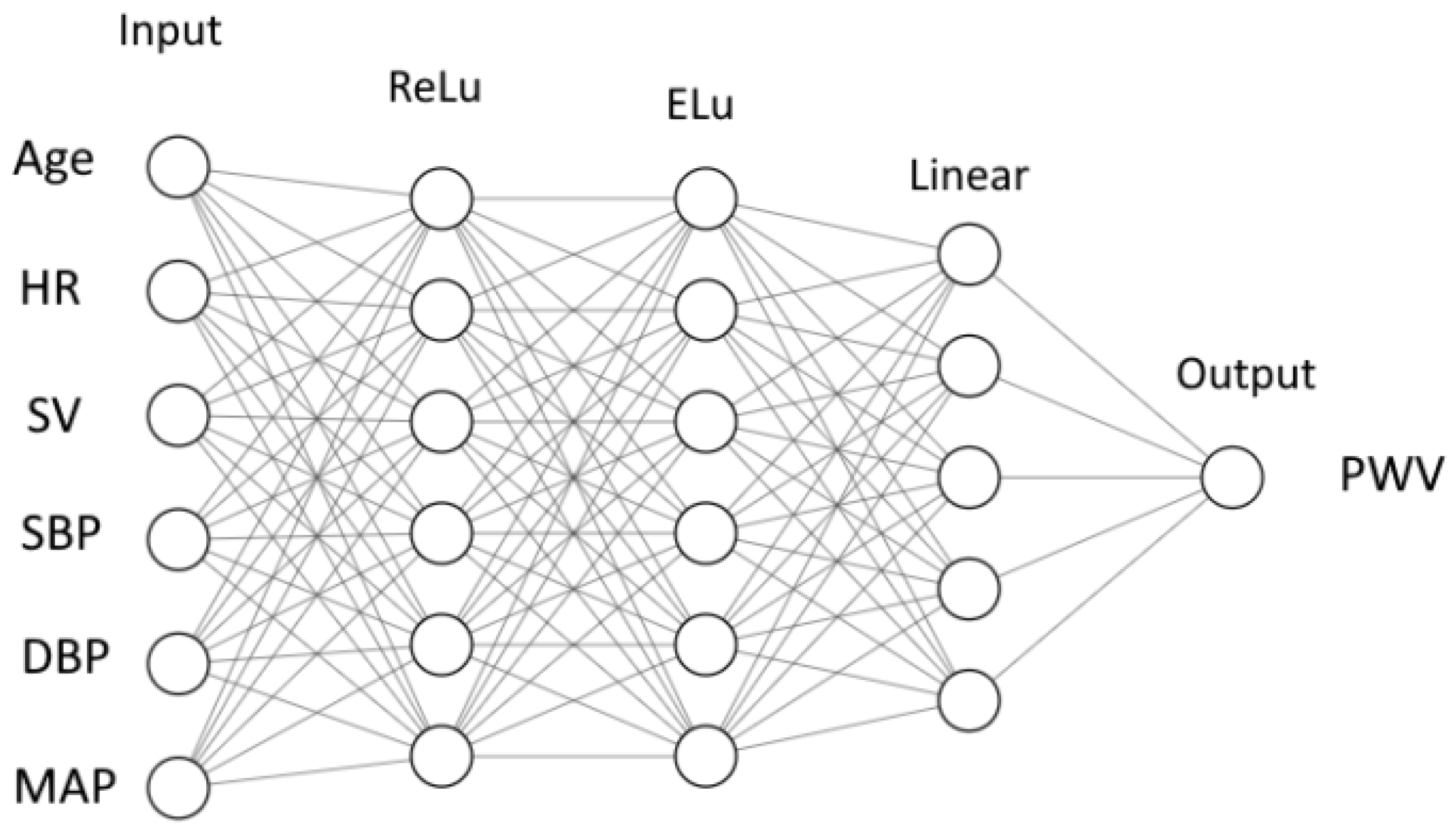
2.4.2. Neural Network

We use a synthetic pulse wave database to train the neural network. We use six input values, including age, HR, SV, brachial systolic blood pressure (SBP), brachial diastolic blood pressure (DBP) and brachial mean blood pressure (MBP). The output can be set to PWV of any major part of systemic circulation presented in the synthetic database. We set the output as the value of brachial–ankle AoPWV, which is measured between the brachial and ankle regions.

We use a feedforward neural network (FNN) [40]. It consists of nodes (neurons). The nodes are grouped in layers. Each neuron collects the outputs from the nodes of the previous layer and produces a single output of its own (Figure 2). An output is computed as a weighted sum of inputs

$$y=w_1{x}_1+w_2{x}_2+w_3{x}_3+\cdots +w_n{x}_n,$$

where y is an output, $x_i$ is the i-th input, $w_i$ is a weight corresponding to the i-th input and n is the number of neurons in the previous layer. The output is calculated as a function of weighted sum

$$y=y\left(s\right),s=w_1{x}_1+w_2{x}_2+w_3{x}_3+\cdots +w_n{x}_n,$$

where $y\left(s\right)$ is called an activation function. Function $y\left(s\right)$ is different for different layers. The case $y\left(s\right)=s$ is referred to as a linear activation function. In this work, we also used standard ReLU and ELU functions. The details of these functions are given in Figure A1.

The weights for each neuron were adjusted during the training procedure. In our case (see Figure 2), we have $2·6·6+5·6+5=107$ weight coefficients, including 2 for the inner layers with 6 neurons and 6 inputs for each neuron, 1 for the inner layer with 5 neurons and 6 inputs for each neuron and output with 5 inputs. We solve the parameter optimization problem using a built-in ADAM optimizer from the PyTorch library. During the training, the data from subjects are processed by a neural network. The final outputs are compared with the target values. The weights are corrected based on the deviations. These corrections occur after a certain number of subjects are processed. The number of subjects between each update is called a ’batch’, and the size of the set is a batch size. One cycle through the full training dataset is called an ’epoch.’ The number of epochs required for training depends on many factors, including the complexity of the neural network, quality of the training dataset, etc.

Thus, the number of inner (hidden) layers, the number of neurons in each layer, the batch size, the number of epochs and the type of activation functions are the parameters to be determined. We optimize these parameters by a hyperparameter tuning algorithm to achieve the lowest error during validation tests on synthetic data. Finally, we set the number of hidden layers to 3, the number of neurons per layer to 6 (to 5 for the last hidden layer), the batch size to 200 and the number of epochs to 150. The activation functions are ReLU, ELU and linear, according to Figure 2. This configuration results in a percentage error of 4–5% during the validation on the synthetic data. However, the same neural network showed a 36% error when tested on the PWV dataset from real patients. We conclude that the resulting neural network is overfitted and apply an early stop technique to avoid overfitting. We break the training process if the percentage error reaches 10%. The value of 10% is chosen on the basis of the repeatability error during PWV measurements [41,42]. It reduces the number of epochs to 11. The updated neural network demonstrates a 16% percentage error during validation on the PWV dataset, which is an acceptable deviation.

We also investigate the performance of the neural network for a various number of layers. For each case, we perform seven runs and calculate the mean values of errors and standard deviations (

Table A1. Comparison of errors for various numbers of hidden layers in the neural network.

Number of Layers	RMSE, m/s	Percentage Error
2 layers	1.55 ± 0.41	19% ± 5%
3 layers	1.31 ± 0.19	16% ± 2%
4 layers	1.32 ± 0.22	16% ± 3%
5 layers	1.37 ± 0.19	17% ± 2%

). It seems that increasing the number of hidden layers beyond three or four does not yield any improvement. We experienced occasional convergence problems during learning: in 1 of 10 runs, the loss function did not decrease a certain large value. In each such case, we restarted the run.

During the FFR simulations, we use the same structure of the neural network, but we train it to estimate actual AoPWV instead of brachial–ankle AoPWV. We train the neural network to produce the same 10% percentage error on synthetic data. We do not have measured values of AoPWV for real patients. Thus, it is impossible to validate the resulting neural network on real measurements. Brachial–ankle AoPWV is a good marker of central aortic stiffness [43] that correlates significantly with AoPWV [44]. Thus, we assume that the neural network trained and validated for brachial–ankle AoPWV can be retrained to estimate AoPWV. We also test the neural networks with various PWV outputs (aortic, brachial–ankle and carotid-femoral). We conclude that neural networks with the same structure and parameters produce a similar error for various types of PWV.

2.4.3. Other Methods

We tested other machine learning methods implemented in the Sklearn library: decision tree, K-nearest neighbors and random forest [45,46]. All methods produce a very low percentage error in synthetic data after hyperparameter tuning. The error of the decision tree is 5%. The error of K-nearest neighbors is 6%. The error of random forest is 4%. Similarly to the developed neural network, all methods perform poorly when tested on the PWV dataset, with percentage errors in the range from 35% to 45%. We tuned the parameters of each method to enforce a 10% error on the synthetic dataset. For the decision tree, we set the maximum depth of the tree to five and imposed a random splitting strategy at each node. For the K-nearest neighbors, we set the number of neighbors to 210 and brute-force search to compute the nearest neighbors and uniform weights for all neighbors. For the random forest, we set the maximum depth of the tree to five and the number of estimators (trees) to five.

3. Results

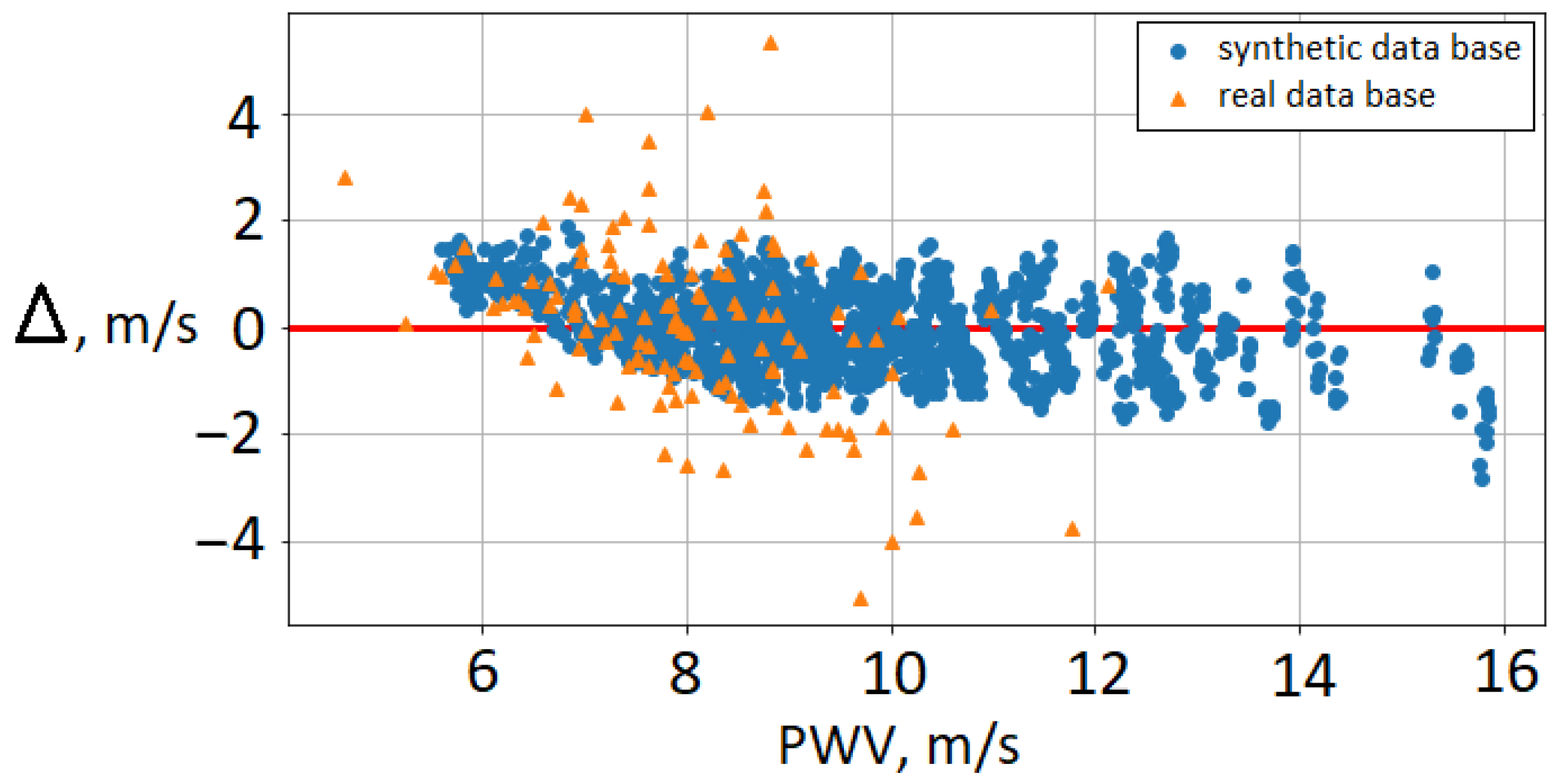
3.1. AoPWV Estimation

Figure 3 shows the difference between brachial–ankle AoPWV predicted with neural network and subjects’ brachial–ankle AoPWV (both for virtual subjects and real patients). We observe that PWV values for real patients tend to be overestimated. RMSE for the PWV dataset is 1.3 m/s, and the percentage error is 16%. In our results, the deviation is higher for female subjects (22%) than for males (14%). The ten patients with the highest deviation were diagnosed with mitral valve insufficiency. Mitral valve pathologies correlate highly with AoPWV [47]. This fact demonstrates the limitations of synthetic databases trained on the basis of the range for a healthy population. Some authors reported that each pathology requires a separate database [15]. Despite these limitations, the developed neural network demonstrated adequate accuracy. It allows the separation of patients into groups with high and low AoPWV to assess the risks of cardiovascular events.

The resulting deviation is close to the reported errors of machine learning methods for AoPWV estimation (Table 2). We compare the 16% percentage error with other similar approaches. These approaches are:

1.

Estimating carotid-femoral PWV from the radial pressure wave using machine learning algorithms [48]. The study population was the Twins UK cohort, containing 3082 subjects aged from 18 to 110 years. The authors used Gaussian process regression and a recurrent neural network to estimate carotid-femoral PWV from the entire radial pressure wave. They report errors of 17–19%.

2.

Estimating carotid-femoral PWV from one carotid waveform measured by tonometry and few clinical variables (age, blood pressure, heart rate, etc.) [48]. The study population included 5050 subjects in the age range of 20 to 69. The authors use the newly developed Intrinsic Frequency algorithm together with neural networks and bootstrap averaging. This algorithm uses an uncalibrated noisy waveform with few additional parameters. The reported error is 14%.

3.

Estimating aortic PWV with ridge regression and a deep neural network from two sets of inputs: a basic set of predictors (age, sex, height, weight, heart rate, systolic and diastolic blood pressure) and an expanded set of predictors (HbA1c, total cholesterol, use of antihypertensive, antidiabetic or cholesterol-lowering medication and smoking status in addition to basic set) [49]. A total of 2254 participants from the Netherlands Epidemiology of Obesity study were included (age 45–65 years). The reported error is 18–22%.

We also compare reported errors with studies devoted to the repeatability of PWV measurements. PWV measurements tend to have a 3–10% variation [41] depending on the method and location of measurement. Another study reports a 10% average difference between two occasionally different measurements of brachial–ankle PWV by one observer. These values give us a good idea of the best possible accuracy. The development of methods with errors below 3–10% would require a substantial improvement in PWV measurement techniques.

We highlight two advantages of our approach. First, developed methods use only six input parameters (Age, SV, HR, SBP, DBP and MBP). It is useful when one does not have much patient-specific data. Secondly, we use synthetic data to train machine learning methods. Collecting large datasets requires extensive amounts of time, workforce and funds. Synthetic databases generated with the help of mathematical models are much cheaper and easier to obtain. They will never be as useful as real datasets, but the availability and flexibility of synthetic data may fit many applications. The shortcomings of our approach are the small validation dataset (PWV dataset) and the focus on brachial–ankle PWV. Brachial–ankle PWV is not as valuable as carotid-femoral PWV or aortic PWV, but it is easier to measure [42].

Table 2. Comparison of various errors in PWV estimation.

Description	Error
Brachial–ankle PWV with a neural network trained on synthetic data ( Table 3. Comparison of different machine learning methods used for AoPWV estimation. For each case, we present the mean values and standard deviations for seven attempts. Method RMSE, m/s Percentage Error K-nearest neighbors 1.96 ± 0.09 24% ± 1% Decision tree 1.88 ± 0.21 23% ± 3% Random forest 1.73 ± 0.14 22% ± 2% Neural network 1.31 ± 0.19 16% ± 2% )	16%
Carotid–femoral PWV with machine learning using peripheral pulse waves [48]	17–19%
Carotid–femoral PWV with a neural network using carotid waveform [50]	14%
Aortic PWV with a neural network [49]	18–22%
The difference between two occasionally different measurements of brachial–ankle PWV by one observer [42]	10%
Repeatability of carotid–femoral PWV measurements [41]	3.4–9.5%

Table 2. Comparison of various errors in PWV estimation.

Description	Error
Brachial–ankle PWV with a neural network trained on synthetic data (Table 3)	16%
Carotid–femoral PWV with machine learning using peripheral pulse waves [48]	17–19%
Carotid–femoral PWV with a neural network using carotid waveform [50]	14%
Aortic PWV with a neural network [49]	18–22%
The difference between two occasionally different measurements of brachial–ankle PWV by one observer [42]	10%
Repeatability of carotid–femoral PWV measurements [41]	3.4–9.5%

Table 3 presents the RMSE and percentage errors for various machine-learning methods. We should consider that the coefficient of variation (ratio between standard deviation and mean value) of brachial–ankle AoPWV is 17% in the PWV dataset and 22% in the synthetic database. It may seem that the performance of the proposed methods is subpar since the percentage error of the three methods is higher than the coefficient of variation for the PWV dataset. However, we trained all methods with a synthetic dataset and did not use any information from the PWV dataset, and we used only six input parameters. Synthetic and real subjects are very different: the synthetic database represents the average healthy population, while the PWV dataset consists of patients with various cardiovascular diseases. This shows that synthetic databases can be used as training datasets when actual patient data are unavailable. In the next section, we demonstrate how the developed methods can be used for parameter identification in cardiovascular simulations.

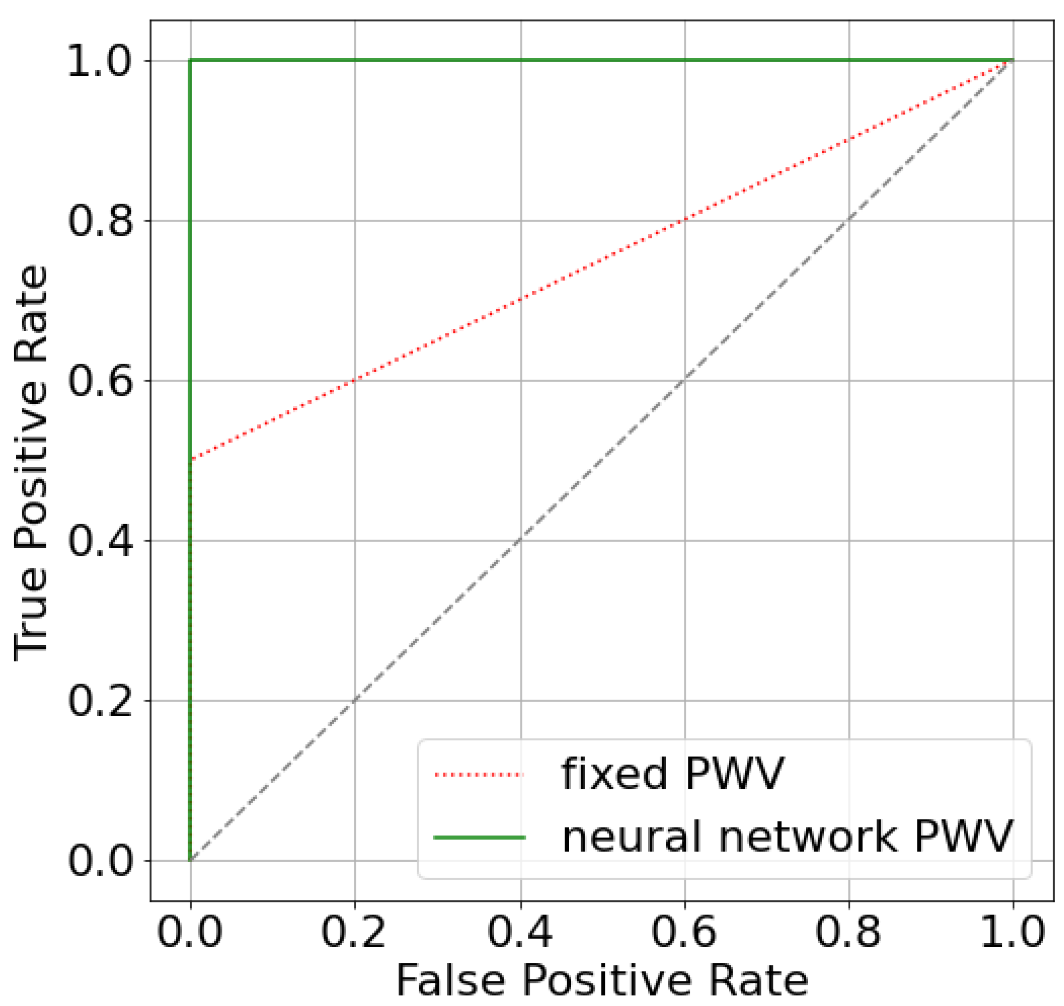
3.2. FFR Estimation with Predicted AoPWV

We present information on each stenosis and invasive FFR measurements in

Table 4. FFR values for average and personalized AoPWV. Vessel ID is the notation of the vessel with stenosis, d is the diameter of the non-stenosed part of a vessel, Degree is the percentage diameter in stenosis, $FF{R}_{inv}$ is the invasively measured FFR value, $cFF{R}_{fixed}$ is the calculated FFR with fixed AoPWV for each case ($AoPWV=7.5$ m/s), $PW{V}_{NN}$ is the AoPWV estimated from the neural network and $cFF{R}_{NN}$ is the calculated FFR with AoPWV estimated from the neural network. The bottom of the table contains the mean values ± standard deviations.

Patient	Vessel ID	d, mm	Degree	${\mathit{FFR}}_{\mathit{inv}}$	${\mathit{cFFR}}_{\mathit{fixed}}$	${\mathit{PWV}}_{\mathit{NN}},\frac{\mathit{m}}{\mathit{s}}$	${\mathit{cFFR}}_{\mathit{NN}}$
1	LAD	1.9	46%	0.89	0.90	9.7	0.89
2	LAD	3.3	61%	0.86	0.87	6.4	0.87
3	RCA	3.0	61%	0.88	0.91	13.5	0.89
4	LAD	2.5	48%	0.82	0.83	8.8	0.83
5	LAD	1.6	55%	0.82	0.81	7.3	0.81
6	LADp	2.4	38%	0.90	0.92	9.1	0.91
6	LADd	2.4	28%	0.82	0.86	9.1	0.85
6	DA	1.9	58%	0.81	0.84	9.1	0.83
7	LAD	1.5	57%	0.75	0.66	7.4	0.66
7	LCX	1.9	32%	0.84	0.85	7.4	0.85
8	LAD	2.3	56%	0.88	0.91	7.8	0.91
8	LCX	3.1	58%	0.89	0.95	7.8	0.95
9	LAD	2.0	48%	0.83	0.89	6.6	0.89
10	LAD	1.9	63%	0.72	0.81	14.2	0.79
		2.2 ± 0.5	51% ± 11%	0.84 ± 0.05	0.86± 0.07	9.1 ± 2.6	0.85 ± 0.07

. The diameters of stenosed vessels and degrees of stenoses are extracted from the post-processed one-dimensional structure of coronary vessels [18]. One can observe that larger vessels with a higher stenosis degree (patients 2 and 3) tend to have higher FFR values. At the same time, narrow vessels with lower stenosis degree (patient 7) tend to have lower FFR values. It demonstrates the well-known fact that the degree of stenosis is not a reliable predictor of possible cardiovascular events [1].

We use the developed neural network to estimate individual values of AoPWV based on datasets from real patients (see Section 2.3). The PWV of coronary vessels (CoPWV) is evaluated as a product of AoPWV and a factor of 1.3 [27,28]. Thus, we personalize both aortic and coronary elasticity: we set parameter c in (4) to be equal to AoPWV or CoPWV. As long as we use the correlation between CoPWV and AoPWV in the rest of the paper, we use AoPWV as an independent parameter. Next, we use these personally predicted $AoPW{V}_{NN}$ values for calculating $cFF{R}_{NN}$ values of each stenosis and compare the results with invasively measured $FF{R}_{inv}$. We also calculated $cFF{R}_{fixed}$ with a fixed default value of $AoPW{V}_{fixed}$ (7.5 m/s) for each stenosis.

The results of the comparison are presented in Table 4. RMSE for calculations with $AoPW{V}_{fixed}$ is ${\sigma }_{fixed}=0.05$. RMSE for calculations with $AoPW{V}_{NN}$ derived by neural network is ${\sigma }_{NN}=0.04$. The average relative deviation improved from $4.4\%$ to $3.8\%$, with a maximum difference of $2.8\%$.

The difference is rather small because only two patients have estimated $AoPW{V}_{NN}$ significantly different from the default $AoPW{V}_{fixed}$ value (patients 3 and 10). We can see that estimating AoPWV from a neural network allowed us to correct the false negative conclusion for patient 10. The simulated value FFR for patient 10 has changed from 0.81 for $AoPW{V}_{fixed}$ to 0.79 for personalized $AoPW{V}_{NN}$ with a possible recommendation for surgical treatment. The latter conclusion conforms with a decision that is based on invasive diagnostics ($FF{R}_{inv}=0.72$). The area under the receiver operator curve (AUC) for both per-vessel and per-patient analysis improved from 0.75 ($AoPW{V}_{fixed}=7.5$ m/s) to 1.0 ($AoPWV$ from a neural network). The improvement of AUC may look significant, but we should consider that the total number of stenoses is 14, and only 2 of them are diagnosed as hemodynamically significant. As a result, ROC-curves only contain two segments (Figure A2). We need a larger set of data to properly analyze the effectiveness of our approach.

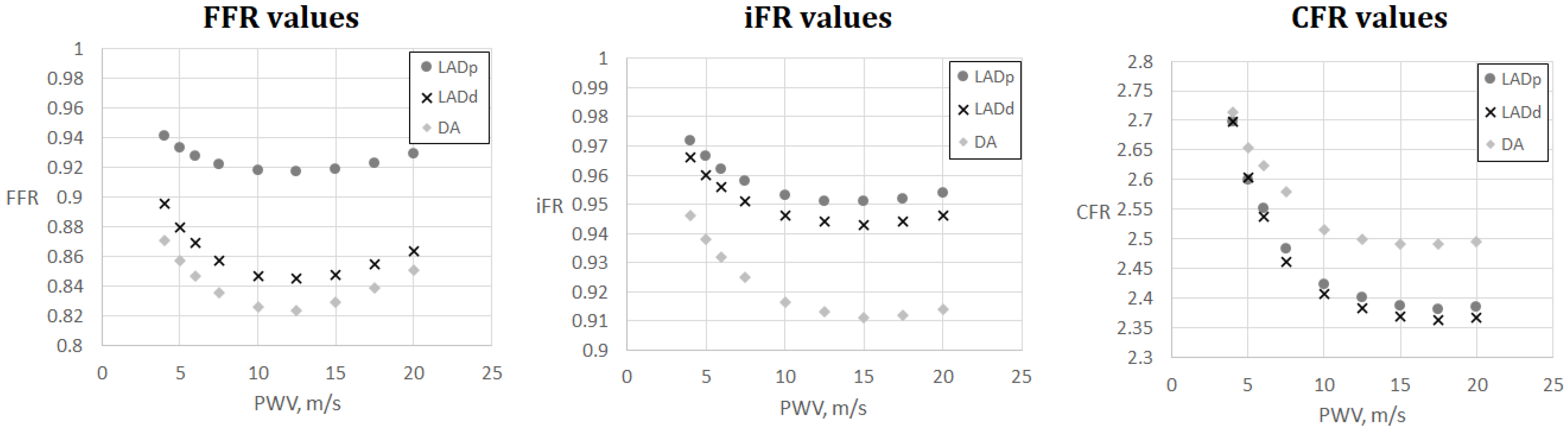
3.3. FFR, iFR and CFR Sensitivity to AoPWV

In Section 3.2, we concluded that a change in AoPWV value modified the predicted FFR value, which slightly decreased below the threshold and provided substantially different clinical recommendations for patient 10. The actual AoPWV value is generally unknown. Although both $FF{R}_{fixed}$ and $FF{R}_{NN}$ differ from the threshold value by $10\%$, it is important to study the sensitivity of FFR and other hemodynamic indices (iFR and CFR) involved in making the clinical decision to AoPWV. It increases the reliability of the conclusions via the evaluation of the possible worst values of the indices, which may be realized outside the clinical conditions or due to the possible errors in parameter evaluation and simulations. Sensitivity analysis also helps in the assessment of the stability of the indices, especially near the threshold. For example, the index may remain within 5–10% below the threshold under various PWV values. Clinicians interpret it as a stable situation, possibly without the need for revascularization.

In this section, we investigate the sensitivity of FFR, iFR and CFR to AoPWV (parameter c in (3)) and identify the critical AoPWV value that corresponds to the minimum value of each index. We performed blood flow simulations for a range of AoPWV values from 4 to 20 m/s with the modified CoPWV. This range covers the physiological values of AoPWV for most patients [25,51]. We set CoPWV to a product of AoPWV and a factor of 1.3 [27,28].

The results are shown in Figure 4, Figure 5, Figure 6 and Figure 7. One can observe that FFR and iFR have increased values for low and high values of AoPWV. CFR values tend to be higher for lower values of AoPWV and almost constant for high AoPWV. The value of AoPWV, which gives a minimum to FFR, iFR and CFR, depends on the particular patient. In our simulations, it ranges from 10 to 12.5 m/s for FFR and iFR and from 12.5 to 20 m/s for CFR. In most cases, CFR is almost constant for AoPWV, greater than 12.5 m/s.

We note the anomalous increase in FFR and iFR with the increase in AoPWV for patient 2 and to a degree for patients 4 and 5 (see Figure 4). Patient 2 had the lowest pressure and the highest cardiac output. Patients 4 and 5 had average values of cardiac output but low blood pressure. This results in a low value of the peripheral resistance (11). FFR sensitivity to AoPWV appears to depend on blood pressure, cardiac output and total peripheral resistance. Total peripheral resistance can be estimated as the ratio between the average blood pressure and cardiac output. Lower values of peripheral resistance result in higher sensitivity for higher values of AoPWV (above 15 m/s).

Figure 5 and Figure 6 demonstrate FFR, iFR and CFR values for patients 6 and 7. These two patients had stenoses of various degrees located in all major branches of LCA (LAD, LCx, DA). Notably, stenosis in DA for patient 6 was the most severe in terms of FFR and iFR but the least severe in terms of CFR. It shows that various hemodynamic indices demonstrate various properties of coronary arteries with stenoses and should be considered together in a complex analysis.

4. Discussion

In this work, we developed a novel machine learning approach to estimate AoPWV. We used a simulated pulse wave database for training and real patients’ data for validation. Based on validation simulations, we report a 16% error and consider it as a promising result. Similar works report a 14–22% error (Table 2). The advantages of our approach are a restricted set of input values and training on synthetic data. These features make our approach more flexible: it is easy to retrain the model to calculate other PWV or add some additional input parameters. We note that the simulated database does not consider possible cardiovascular pathologies. Our approach may be improved by including more input parameters and refining the neural network structure. Expanding the simulated pulse wave database and incorporating various pathologies is another way to increase accuracy. This improvement is labor-intensive and time-consuming due to the exponential growth of the complexity of virtual databases with each new variable parameter.

The hemodynamic parameters’ sensitivity to AoPWV is rather low. The length and the degree of stenosis are much more important factors. Nevertheless, transient (close to threshold) values of the FFR, iFR and CFR can change the diagnosis due to the corrected AoPWV value. The developed approach for AoPWV identification can be used for the evaluation of the other parameters as well. For example, stroke volume or peripheral resistance can be estimated similarly.

This study shows that hemodynamic indices undergo substantial change within the range of AoPWV below 12 m/s, which corresponds to a more elastic vasculature. Our simulations showed that these cases correspond to the highest values of FFR, iFR and CFR. More elastic vessels adapt to the increase in blood flow [52] and thus, the hemodynamic significance of their stenosis is lower. Clinical studies also show that FFR is higher in more flexible vasculature [53]. Higher values of AoPWV correspond to stiffer vessels, which become similar to the rigid tubes. It explains almost constant values of CFR for AoPWV greater than 15 m/s. The ratio between hyperemic and resting flows mainly on peripheral resistance since the diameters in all cases are almost identical. FFR and iFRs represent the ratios of pressures. Elevation of AoPWV increases the pressure in both numerator and denominator. As a result, both FFR and iFR increase.

Summarizing the results of the simulations, we conclude that hemodynamic significance of the stenosis is higher for patients with AoPWV in the range from 10 to 15 m/s. Of course, this needs further confirmation by clinical studies.

References

1. Götberg, M.; Christiansen, E.H.; Gudmundsdottir, I.J.; Sandhall, L.; Danielewicz, M.; Jakobsen, L.; Olsson, S.E.; Öhagen, P.; Olsson, H.; Omerovic, E.; et al. Instantaneous wave-free ratio versus fractional flow reserve to guide PCI. N. Engl. J. Med. 2019, 376, 1813–1823. [Google Scholar] [CrossRef] [PubMed] [Green Version]
2. Gould, K.L.; Kirkeeide, R.L.; Buchi, M. Coronary flow reserve as a physiologic measure of stenosis severity. J. Am. Coll. Cardiol. 1990, 15, 459–474. [Google Scholar] [CrossRef] [PubMed] [Green Version]
3. Carson, J.M.; Pant, S.; Roobottom, C.; Alcock, R.; Blanco, P.J.; Carlos Bulant, C.A.; Vassilevski, Y.; Simakov, S.; Gamilov, T.; Pryamonosov, R.; et al. Non-invasive coronary CT angiography-derived fractional flow reserve: A benchmark study comparing the diagnostic performance of four different computational methodologies. Int. J. Numer. Methods Biomed. Eng. 2019, 35, e3235. [Google Scholar] [CrossRef] [PubMed] [Green Version]
4. Carson, J.M.; Roobottom, C.; Alcock, R.; Nithiarasu, P. Computational instantaneous wave-free ratio (IFR) for patient-specific coronary artery stenoses using 1D network models. Int. J. Numer. Methods Biomed. Eng. 2019, 35, e3255. [Google Scholar] [CrossRef] [Green Version]
5. Simakov, S.; Gamilov, T.; Liang, F.; Kopylov, P. Computational analysis of haemodynamic indices in synthetic atherosclerotic coronary netwroks. Mathematics 2021, 9, 2221. [Google Scholar] [CrossRef]
6. Gognieva, D.; Mitina, Y.; Gamilov, T.; Pryamonosov, R.; Vasilevskii, Y.; Simakov, S.; Liang, F.; Ternovoy, S.; Serova, N.; Tebenkova, E.; et al. Noninvasive assessment of the fractional flow reserve with the CT FFRc 1D method: Final results of a pilot study. Glob. Heart 2020, 16, 837. [Google Scholar] [CrossRef]
7. Zheng, D.; Weiwei, C.; Hao, G.; Xilan, Y.; Xiaoyu, L.; Nicholas, A.H. A One-Dimensional Hemodynamic Model of the Coronary Arterial Tree. Front. Physiol. 2019, 10, 853. [Google Scholar]
8. Mynard, J.P.; Penny, D.J.; Smolich, J.J. Scalability and in vivo validation of a multiscale numerical model of the left coronary circulation. Am. J. Physiol. Heart Circ. 2014, 306, H517–H528. [Google Scholar] [CrossRef]
9. Kamangar, S.; Badruddin, I.A.; Govindaraju, K.; Nik-Ghazali, N.; Badarudin, A.; Viswanathan, G.N.; Ahmed, N.; Khan, T. Patient-specific 3D hemodynamics modelling of left coronary artery under hyperemic conditions. Med. Biol. Eng. Comput. 2017, 55, 1451–1461. [Google Scholar] [CrossRef]
10. Lu, M.T.; Ferencik, M.; Roberts, R.S.; Lee, K.L.; Ivanov, A.; Adami, E.; Mark, D.B.; Jaffer, F.A.; Leipsic, J.A.; Douglas, P.S.; et al. Noninvasive FFR Derived From Coronary CT Angiography: Management and Outcomes in the PROMISE Trial. JACC Cardiovasc. Imaging 2017, 10, 1350–1358. [Google Scholar] [CrossRef]
11. Charlton, P.H.; Mariscal Harana, J.; Vennin, S.; Li, Y.; Chowienczyk, P.; Alastruey, J. Modeling arterial pulse waves in healthy aging: A database for in silico evaluation of hemodynamics and pulse wave indexes. Am. J.-Physiol.-Heart Circ. Physiol. 2019, 317, H1062–H1085. [Google Scholar] [CrossRef] [PubMed] [Green Version]
12. Charlton, P.H. Pulse Wave Database. Available online: https://peterhcharlton.github.io/pwdb/pwdb.html (accessed on 23 February 2023).
13. Reavette, R.M.; Sherwin, S.J.; Tang, M.; Weinberg, P.D. Comparison of arterial wave intensity analysis by pressure-velocity and diameter-velocity methods in a virtual population of adult subjects. Proc. Inst. Mech. Eng. H 2020, 234, 1260–1276. [Google Scholar] [CrossRef] [PubMed]
14. Jones, G.; Parr, J.; Nithiarasu, P.; Pant, S. A physiologically realistic virtual patient database for the study of arterial haemodynamics. Int. J. Numer. Method Biomed. Eng. 2021, 37, e3497. [Google Scholar] [CrossRef] [PubMed]
15. Wang, T.; Jin, W.; Liang, F.; Alastruey, J. Machine Learning–Based Pulse Wave Analysis for Early Detection of Abdominal Aortic Aneurysms Using In Silico Pulse Waves. Symmetry 2021, 13, 804. [Google Scholar] [CrossRef]
16. Carson, J.M.; Chakshu, N.K.; Sazonov, I.; Nithiarasu, P. Artificial intelligence approaches to predict coronary stenosis severity using non-invasive fractional flow reserve. Proc. Inst. Mech. Eng. H 2020, 234, 1337–1350. [Google Scholar] [CrossRef]
17. Fossan, F.E.; Müller, L.O.; Sturdy, J.; Barten, A.T.; Jørgensen, A.; Wiseth, R.; Hellevik, L.R. Machine learning augmented reduced-order models for FFR-prediction. Comput. Methods Appl. Mech. Eng. 2021, 384, 113892. [Google Scholar] [CrossRef]
18. Danilov, A.; Ivanov, Yu.; Pryamonosov, R.; Vassilevski, Yu. Methods of graph network reconstruction in personalized medicine. Int. J. Numer. Methods Biomed. Eng. 2016, 32, e02754. [Google Scholar] [CrossRef]
19. Vassilevski, Y.V.; Salamatova, V.Y.; Simakov, S.S. On the elasticity of blood vessels in one-dimensional problems of haemodynamics. Comput. Math. Math. Phys. 2015, 55, 1567–1578. [Google Scholar] [CrossRef]
20. Simakov, S.; Gamilov, T.; Liang, F.; Gognieva, D.G.; Gappoeva, M.K.; Kopylov, P.Y. Numerical evaluation of the effectiveness of coronary revascularization. Russ. J. Num. Anal. Math. Mod. 2021, 36, 303–312. [Google Scholar] [CrossRef]
21. Matthys, K.S.; Alastruey, J.; Peiro, J.; Khir, A.W.; Segers, P.; Verdonck, P.R.; Parker, K.H.; Sherwin, S.J. Pulse wave propagation in a model human arterial network: Assessmentof 1D numerical simulations against in-vitro measurements. J. Biomech. 2007, 40, 3476–3486. [Google Scholar] [CrossRef]
22. Milan, A.; Zocaro, G.; Leone, D.; Tosello, F.; Buraioli, I.; Schiavone, D.; Veglio, F. Current assessment of pulse wave velocity: Comprehensive review of validation studies. J. Hypertens. 2019, 37, 1547–1557. [Google Scholar] [CrossRef] [PubMed]
23. Pereira, T.; Correia, C.; Cardoso, J. Novel Methods for Pulse Wave Velocity Measurement. J. Med. Biol. Eng. 2015, 35, 555–565. [Google Scholar] [CrossRef] [PubMed] [Green Version]
24. Filip, C.; Cirstoveanu, C.; Bizubac, M.; Berghea, E.C.; Căpitănescu, A.; Bălgrădean, M.; Pavelescu, C.; Nicolescu, A.; Ionescu, M.D. Pulse Wave Velocity as a Marker of Vascular Dysfunction and Its Correlation with Cardiac Disease in Children with End-Stage Renal Disease (ESRD). Diagnostics 2021, 12, 71. [Google Scholar] [CrossRef] [PubMed]
25. Shahzad, R.; Shankar, A.; Amier, R.; Nijveldt, R.; Westenberg, J.J.M.; de Roos, A.; Lelieveldt, B.P.F.; van der Geest, R.J. Quantification of aortic pulse wave velocity from a population based cohort: A fully automatic method. J. Cardiovasc. Magn. Reson. 2019, 21, 27. [Google Scholar] [CrossRef] [Green Version]
26. Van Hout, M.J.; Dekkers, I.A.; Westenberg, J.J.; Schalij, M.J.; Widya, R.L.; de Mutsert, R.; Rosendaal, F.R.; de Roos, A.; Jukema, J.W.; Scholte, A.J.; et al. Normal and reference values for cardiovascular magnetic resonance-based pulse wave velocity in the middle-aged general population. J. Cardiovasc. Magn. Reson. 2021, 23, 46. [Google Scholar] [CrossRef]
27. Aguado-Sierra, J.; Parke, K.H.; Davies, J.E.; Francis, D.; Hughes, A.D.; Mayet, J. Arterial pulse wave velocity in coronary arteries. In Proceedings of the 2006 International Conference of the IEEE Engineering in Medicine and Biology Society, New York, NY, USA, 30 August–3 September 2006; pp. 867–870. [Google Scholar]
28. Harbaoui, B.; Courand, P.-Y.; Cividjian, A.; Lantelme, P. Development of Coronary Pulse Wave Velocity: New Pathophysiological Insight Into Coronary Artery Disease. J. Am. Heart Assoc. 2017, 6, e004981. [Google Scholar] [CrossRef]
29. Barret, K.; Brooks, H.; Boitano, S.; Barman, S. Ganong’s Review of Medical Physiology, 23rd ed.; The McGraw-Hill: New York, NY, USA, 2010. [Google Scholar]
30. Gamilov, T.; Kopylov, P.; Serova, M.; Syunaev, R.; Pikunov, A.; Belova, S.; Liang, F.; Alastruey, J.; Simakov, S. Computational analysis of coronary blood flow: The role of asynchronous pacing and arrhythmias. Mathematics 2020, 8, 1205. [Google Scholar] [CrossRef]
31. Magomedov, K.M.; Kholodov, A.S. Grid–Characteristic Numerical Methods; Nauka: Moscow, Russia, 2018. (In Russian) [Google Scholar]
32. Ernest, W.L.; Menezes, L.J.; Torii, R. On outflow boundary conditions for CT-based computation of FFR: Examination using PET images. Med. Eng. Phys. 2020, 76, 79–87. [Google Scholar]
33. Pijls, N.H.J.; de Bruyne, B.; Peels, K.; van der Voort, P.H.; Bonnier, H.J.R.M.; Bartunek, J.; Koolen, J.J. Measurement of Fractional Flow Reserve to Assess the Functional Severity of Coronary-Artery Stenoses. N. Engl. J. Med. 1996, 334, 1703–1708. [Google Scholar] [CrossRef]
34. Nijjer, S.S.; Sen, S.; Petraco, R.; Sachdeva, R.; Cuculi, F.; Escaned, J.; Broyd, C.; Foin, N.; Hadjiloizou, N.; Foale, R.A.; et al. Improvement in coronary haemodynamics after percutaneous coronary intervention: Assessment using instantaneous wave-free ratio. Heart 2013, 99, 1740–1748. [Google Scholar] [CrossRef] [Green Version]
35. Sen, S.; Escaned, J.; Malik, I.S.; Mikhail, G.W.; Foale, R.A.; Mila, R.; Tarkin, J.; Petraco, R.; Broyd, C.; Jabbou, R.; et al. Development and validation of a new adenosine–independent index of stenosis severity from coronary wave-intensity analysis: Results of the ADVISE (ADenosine Vasodilator Independent Stenosis Evaluation) study. J. Am. Coll. Cardiol. 2012, 59, 1392–1402. [Google Scholar] [CrossRef] [PubMed] [Green Version]
36. Carson, J.; Pant, S.; Roobottom, C.; Alcock, R.; Blanco, P.J.; Bulant, C.A.; Vassilevski, Y.; Simakov, S.; Gamilov, T.; Pryamonosov, R.; et al. Supplementary Material. 2019. Available online: https://doi.org/10.6084/m9.figshare.8047742.v2 (accessed on 23 February 2023). [CrossRef]
37. Laurent, S.; Boutouyrie, P.; Asmar, R.; Gautier, I.; Laloux, B.; Guize, L.; Ducimetiere, P.; Benetos, A. Aortic stiffness is an independent predictor of all-cause and cardiovascular mortality in hypertensive patients. Hypertension 2001, 37, 1236–1241. [Google Scholar] [CrossRef] [PubMed] [Green Version]
38. Munakata, M. Brachial-Ankle Pulse Wave Velocity: Background, Method, and Clinical Evidence. Pulse 2016, 3, 195–204. [Google Scholar] [CrossRef] [Green Version]
39. Collis, T.; Devereux, R.B.; Roman, M.J.; de Simone, G.; Yeh, J.; Howard, B.V.; Fabsitz, R.R.; Welty, T.K. Relations of stroke volume and cardiac output to body composition: The strong heart study. Circulation 2001, 103, 820–825. [Google Scholar] [CrossRef] [PubMed] [Green Version]
40. Schmidhuber, J. Deep learning in neural networks: An overview. Neural Netw. 2015, 61, 85–117. [Google Scholar] [CrossRef] [Green Version]
41. Grillo, A.; Parati, G.; Rovina, M.; Moretti, F.; Salvi, L.; Gao, L.; Baldi, C.; Sorropago, G.; Faini, A.; Millasseau, S.; et al. Short-Term Repeatability of Noninvasive Aortic Pulse Wave Velocity Assessment: Comparison Between Methods and Devices. Am. J. Hypertens. 2018, 31, 80–88. [Google Scholar] [CrossRef]
42. Yamashina, A.; Tomiyama, H.; Takeda, K.; Tsuda, H.; Arai, T.; Hirose, K.; Koji, Y.; Hori, S.; Yamamoto, Y. Validity, reproducibility, and clinical significance of noninvasive brachial-ankle pulse wave velocity measurement. Hypertens. Res. 2002, 25, 359–364. [Google Scholar] [CrossRef] [Green Version]
43. Kang, J.; Kim, H.L.; Lim, W.H.; Seo, J.B.; Zo, J.H.; Kim, M.A.; Kim, S.H. Relationship between brachial-ankle pulse wave velocity and invasively measured aortic pulse pressure. J. Clin. Hypertens. 2018, 20, 462–468. [Google Scholar] [CrossRef] [Green Version]
44. Sugawara, J.; Hayashi, K.; Yokoi, T.; Cortez-Cooper, M.Y.; DeVan, A.E.; Anton, M.A.; Tanaka, H. Brachial–ankle pulse wave velocity: An index of central arterial stiffness? J. Hum. Hypertens 2005, 19, 401–406. [Google Scholar] [CrossRef] [Green Version]
45. Mahesh, B. Machine Learning Algorithms—A Review. Int. J. Sci. Res. 2020, 9, 381–386. [Google Scholar]
46. Dietterich, T. An Experimental Comparison of Three Methods for Constructing Ensembles of Decision Trees: Bagging, Boosting, and Randomization. Mach. Learn. 2000, 40, 139–157. [Google Scholar] [CrossRef]
47. Rossi, A.; Bonapace, S.; Cicoira, M.; Conte, L.; Anselmi, A.; Vassanelli, C. Aortic stiffness: An old concept for new insights into the pathophysiology of functional mitral regurgitation. Heart Vessel. 2013, 28, 606–612. [Google Scholar] [CrossRef] [PubMed]
48. Jin, W.; Chowienczyk, P.; Alastruey, J. Estimating pulse wave velocity from the radial pressure wave using machine learning algorithms. PLoS ONE 2021, 16, e0245026. [Google Scholar] [CrossRef] [PubMed]
49. Van Hout, M.J.; Dekkers, I.A.; Lin, L.; Westenberg, J.J.; Schalij, M.J.; Jukema, J.W.; Widya, R.L.; Boone, S.C.; de Mutsert, R.; Rosendaal, F.R.; et al. Estimated pulse wave velocity (ePWV) as a potential gatekeeper for MRI-assessed PWV: A linear and deep neural network based approach in 2254 participants of the Netherlands Epidemiology of Obesity study. Int. J. Cardiovasc. Imaging 2022, 38, 183–193. [Google Scholar] [CrossRef] [PubMed]
50. Tavallali, P.; Razavi, M.; Pahlevan, N.M. Artificial Intelligence Estimation of Carotid-Femoral Pulse Wave Velocity using Carotid Waveform. Sci. Rep. 2018, 8, 1014. [Google Scholar] [CrossRef] [Green Version]
51. Sutton-Tyrrell, K.; Mackey, R.H.; Holubkov, R.; Vaitkevicius, P.V.; Spurgeon, H.A.; Lakatta, E.G. Measurement variation of aortic pulse wave velocity in the elderly. Am. J. Hypertens. 2001, 14, 463–468. [Google Scholar] [CrossRef] [Green Version]
52. Yong, A.S.C.; Javadzadegan, A.; Fearon, W.F.; Moshfegh, A.; Lau, J.K.; Nicholls, S.; Ng, M.K.C.; Kritharides, L. The relationship between coronary artery distensibility and fractional flow reserve. PLoS ONE 2017, 12, e0181824. [Google Scholar] [CrossRef] [Green Version]
53. Cividjian, A.; Harbaoui, B.; Chambonnet, C.; Bonnet, J.M.; Paquet, C.; Courand, P.Y.; Lantelme, P. Comprehensive assessment of coronary pulse wave velocity in anesthetized pigs. Physiol. Rep. 2020, 8, e14424. [Google Scholar] [CrossRef]
Figure 1. The structure of the computational domain for patient 1. LCA and RCA were extracted from the patient’s CT scans. Each numbered segment corresponds in the model to a one-dimensional tube. Stenosis is a separate segment with decreased diameter. We solve hyperbolic set (1) in the inner points of each segment. We impose mass conservation (5) and continuity of the total pressure (6) on each junction. FFR is measured at segment 6.
Mathematics 11 01358 g001
Figure 2. Structure of neural network: inputs, output, layers, number of neurons in each layer and activation functions (ReLu, ELu and Linear—Figure A1).
Mathematics 11 01358 g002
Figure 3. Bland–Altman plot for brachial–ankle AoPWV: cross-validation on the synthetic database (blue circles) and comparison with brachial–ankle AoPWV calculated for real patients (orange triangles). Δ —difference between brachial–ankle AoPWV predicted by the neural network and subject’s brachial–ankle AoPWV.
Mathematics 11 01358 g003
Figure 4. FFR, iFR and CFR sensitivity to AoPWV for patients from 1 to 5.
Mathematics 11 01358 g004
Figure 5. FFR, iFR and CFR sensitivity to AoPWV for patient 6. Patient 6 had three stenoses located in the proximal part of the left anterior descending artery (LADp), distal part of the left anterior descending artery (LADd) and middle part of the diagonal artery (DA).
Mathematics 11 01358 g005
Figure 6. FFR, iFR and CFR sensitivity to AoPWV for patient 7. Patient 7 had two stenoses located in the left anterior descending artery (LAD) and the left circumflex artery (LCx).
Mathematics 11 01358 g006
Figure 7. FFR, iFR and CFR sensitivity to AoPWV for patients from 8 to 10. Patient 8 had two stenoses located in the left anterior descending artery (LAD) and the left circumflex artery (LCx).
Mathematics 11 01358 g007