Predefined-Time (PDT) Synchronization of Impulsive Fuzzy BAM Neural Networks with Stochastic Perturbations

Abstract

This paper focuses on the predefined-time (PDT) synchronization issue of impulsive fuzzy bidirectional associative memory neural networks with stochastic perturbations. Firstly, useful definitions and lemmas are introduced to define the PDT synchronization of the considered system. Next, a novel controller with a discontinuous sign function is designed to ensure the synchronization error converges to zero in the preassigned time. However, the sign function may cause the chattering effect, leading to undesirable results such as the performance degradation of synchronization. Hence, we designed a second novel controller to eliminate this chattering effect. After that, we obtained some sufficient conditions to guarantee the PDT synchronization of the drive–response systems by using the Lyapunov function method. Finally, three numerical simulations are provided to evaluate the validity of the theoretical results.

1. Introduction

Since bidirectional associative memory (BAM) neural network was first introduced by Kosko in 1987 [1,2], it has been widely studied due to its applicability in many fields, such as pattern recognition [3], computer-assisted learning in chemistry [4], signal processing [5], image processing [6], and other areas. Thus, it is necessary to research the stability and synchronization of chaotic nonlinear systems for their significant role in the above mentioned fields [7,8]. As shown in Figure 1, it is easy to see that, BAM neural networks are constructed by two layers of interconnected neurons [3], and this kind of structure means that BAM neural networks possess hyper-chaotic attractors.In the last decade, many studies have been conducted on the dynamical behavior analysis of BAM neural networks with or without fuzzy logic, with or without stochastic perturbations, and with or without impulse. For instance, Cao et al. studied the global asymptotic stability of delayed BAM neural networks by using the Lyapunov method [9]. In [10], the authors investigated the synchronization of memristor-based BAM neural networks by using the linear matrix inequality technique. In [11], the authors investigated the general decay synchronization of time-delayed BAM neural networks by designing a nonlinear feedback controller. However, most of the works are about infinite-time synchronization. Recently, scholars found that the convergence time of synchronization is an important issue because of its applicability in the field of engineering [12]. The finite-time (FNT) synchronization error can converge to zero in finite time. Furthermore, FNT synchronization has a faster convergence rate than infinite-time synchronization [13,14,15]. Polyakov, in [16], introduced fixed-time (FXT) synchronization in order to resolve the issue of the settling time (ST) of FNT extensively relying on initial values. A number of research works on FXT synchronization have been published in recent years [17,18]. There is no doubt that FXT synchronization has its drawbacks as well as merits, such as its ST still being relevant to the system parameters, and that the convergence time cannot be predicted in advance. Hence, it is a necessary task to analyze whether a nonlinear system can reach complete synchronization within a predefined-time (PDT). This has led to the development of a novel synchronization technique called PDT synchronization. The importance of this synchronization method lies in the fact that its ST can be determined according to needs. Recent studies have investigated this challenging research topic [19,20,21].

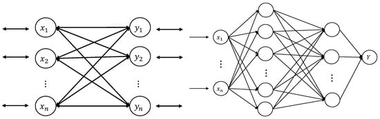
Figure 1. The construction of BAM neural networks (left) and fuzzy min-max neural networks (right).

In many dynamical systems, fuzziness often is inevitable. Thus, the study of fuzziness in neural networks has attracted great interest over recent years. Yang et al. combined fuzzy logic with cellular networks (CNNs), and introduced fuzzy cellular networks (FCNNs) [22,23]. The construction of fuzzy min-max networks is shown in Figure 1, and for specific information refer to [24]. In [25], the authors introduced decentralized event-triggering control for the finite-time boundedness of FCNNs during a cyber-attack. FCNNs can be applied in pattern recognition and image processing techniques [26,27]. Synchronization is the most significant dynamic behavior of neural networks. Thus, there are many works that explore the synchronization of FCNNs [28,29,30,31]. For example, in [28], the authors investigated the robust synchronization of a chaotic system under fuzzy controllers. Finite-time synchronization for TS fuzzy complex dynamical networks has been considered in [30]. Duan et al. investigated the FXT synchronization neural-type BAM memristive-inertial neural networks with fuzzy logic [31].

In addition, the synchronization of neural networks with stochastic perturbations has recently attracted interest in the research community, mainly because many systems are unavoidably affected by noise and stochastic disturbance [32]. In recent years, scholars have conducted much research on the synchronization of stochastic BAM neural networks with or without fuzziness, and with or without the destabilizing impulse [19,20,33,34,35]. For example, in [20,34,35], the authors investigated FNT synchronization and FXT/PDT synchronization, respectively, for stochastic BAM neural networks and obtained novel results. In [20], the authors successfully combined the destabilizing impulse with stochastic perturbations, and obtained an ST estimation for a general impulsive system.

In [21], the authors considered the FXT/PDT stability of fuzzy neural networks with stochastic perturbations. However, the research on impulsive fuzzy BAM neural networks with stochastic perturbations is scarce. Motivated by the observations outlined above, in this paper, we consider the PDT synchronization of stochastic fuzzy impulsive BAM neural networks. The main contributions of this paper are as follows: Firstly, this is the first study to consider the PDT synchronization of BAM neural networks with stochastic perturbations, fuzzy logic and impulsive effects. Secondly, some simple PDT synchronization criteria for BAM neural networks with stochastic perturbations, fuzzy logic and general impulsive effects are designed with novel controllers. Thirdly, PDT synchronization is independent of the parameter sets and initial conditions.

We have organized the rest of this paper as follows. In the second section, some useful definitions, lemmas and the details of the considered systems will be introduced. They are important for proving the main results in the following section. In the third section, we present the design for novel controllers with and without a discontinuous sign function for the PDT synchronization of impulsive fuzzy BAM neural networks with stochastic perturbations. In the fourth section, we provide three examples to evaluate the effectiveness of the theoretical results of this paper. In the final section, we summarize this paper by providing a brief conclusion.

2. System Description and Preliminary Knowledge

Here, we consider the following fuzzy impulsive BAM neural networks with stochastic perturbations,

$$\left\{\begin{array}{cc}\hfill d{x}_i(t)=& [-a_i{x}_i(t)+\sum _{j=1}^m{b}_{ij}{h}_j(y_j(t))+\underset{j=1}{\overset{m}{\bigwedge }}{T}_{ij}{\nu }_j+\underset{j=1}{\overset{m}{\bigwedge }}{\alpha }_{ij}{h}_j(y_j(t))\hfill \\ \hfill & +\underset{j=1}{\overset{m}{\bigvee }}{S}_{ij}{\nu }_j+\underset{j=1}{\overset{m}{\bigvee }}{\beta }_{ij}{h}_j(y_j(t))+I_i]dt+{\varrho }_i(t,x_i(t))d\omega (t),t\ne t_{\tau },\hfill \\ \hfill d{y}_j(t)=& [-{\overline{a}}_j{y}_j(t)+\sum _{i=1}^n{\overline{b}}_{ji}{g}_i(x_i(t))+\underset{i=1}{\overset{n}{\bigwedge }}{T}_{ji}{\overline{\nu }}_i+\underset{i=1}{\overset{n}{\bigwedge }}{\overline{\alpha }}_{ji}{g}_i(x_i(t))\hfill \\ \hfill & +\underset{i=1}{\overset{n}{\bigvee }}{S}_{ji}{\overline{\nu }}_i+\underset{i=1}{\overset{n}{\bigvee }}{\overline{\beta }}_{ji}{g}_i(x_i(t))+J_j]dt+{\overline{\varrho }}_j(t,y_j(t))d\omega (t),t\ne t_{\tau },\hfill \\ \hfill \Delta x_i(t_{\tau })& =x_i(t_{\tau }^{+})-x_i(t_{\tau }^{-})=({\xi }_i-1)x_i(t_{\tau }),\hfill \\ \hfill \Delta y_j(t_{\tau })& =y_j(t_{\tau }^{+})-y_j(t_{\tau }^{-})=({\zeta }_j-1)y_j(t_{\tau }),\hfill \end{array}\right.$$

(1)

where $\tau \in N,i\in \mathcal{I}\triangleq \{1,2,\dots ,n\},j\in \mathcal{J}\triangleq \{1,2,\dots ,m\}$, and n and m are the number of neurons of the neural fields $X_U$ and $Y_U$, respectively. $x_i(t)\in R$ and $y_j(t)\in R$ correspond to the state variables of the ith neuron of $X_U$ and jth neuron of $Y_U$ at time t, respectively. Positive constants $a_i$ and ${\overline{a}}_j$ stand for the self-inhibition rate of the ith neuron of $X_U$ and jth neuron of $Y_U$, respectively. Constants $b_{ij}$ and ${\overline{b}}_{ji}$ represent the synaptic connection weights. ⋁ and ⋀ are the fuzzy OR and AND operations, respectively. ${\alpha }_{ij}$ and ${\overline{\alpha }}_{ij}$, ${\beta }_{ij}$ and ${\overline{\beta }}_{ij}$ denote the fuzzy feedback MIN and MAX template, respectively. $T_{ij}$ and $S_{ij}$ represent the elements of the fuzzy feed-forward MIN and MAX template, respectively. $I_i$ and $J_J$, ${\overline{\nu }}_i$ and ${\nu }_j$ are the bias and input of the ith neuron of $X_U$ and jth neuron of $Y_U$, respectively. $h_j(·)$ and $g_i(·)$ correspond to neuron activation functions. ${\varrho }_i(t,·):R^{+}\times R\to R$ and ${\overline{\varrho }}_j(t,·):R^{+}\times R\to R$ represent the noise intensity functions. $\omega (t)$ is a one dimensional Brownian motion provided on a complete probability space $(\Omega ,F,P)$ with a natural filtration ${\{F_t\}}_t\ge 0$ generated by $\omega (t)$. ${\xi }_i$ and ${\zeta }_j$ are positive constants. $x_i(t_{\tau }^{-})\to x_i(t_{\tau })$ and $y_j(t_{\tau }^{-})\to y_j(t_{\tau })$ as $t\to t_{\tau -0}$, $x_i(t_{\tau }^{+})={lim}_{t\to t_{\tau +0}}{x}_i(t)$, $y_i(t_{\tau }^{+})={lim}_{t\to t_{\tau +0}}{y}_i(t)$, for all $\tau \in N$, stand for the jumps at the impulse moment $t_{\tau }$, and $\{t_{\tau },\tau =1,2,\dots \}$ is a strictly increasing sequence such that ${lim}_{\tau \to +\infty }{t}_{\tau }=+\infty$. The initial conditions of system (1) are as follows:

$$\begin{array}{cc}\hfill & x_i(0)=x_i^0,i\in \mathcal{I},\hfill \\ \hfill & y_j(0)=y_j^0,j\in \mathcal{J}.\hfill \end{array}$$

Throughout the paper, we assume that

Assumption 1.

For any $i\in \mathcal{I}$, $j\in \mathcal{J}$, the neuron activation functions $h_j(·)$ and $g_i(·)$ satisfy the Lipschitz condition; that is, for all ${\mu }_1,{\mu }_2\in R$, there exist positive constants $L_j^h$ and $L_i^g$ such that

$$\begin{array}{cc}\hfill & |h_j({\mu }_1)-h_j({\mu }_2)|\le L_j^h|{\mu }_1-{\mu }_2|,\hfill \\ \hfill & |g_i({\mu }_1)-g_i({\mu }_2)|\le L_i^g|{\mu }_1-{\mu }_2|.\hfill \end{array}$$

Assumption 2.

For any $i\in \mathcal{I}$, $j\in \mathcal{J}$, the noise intensity functions ${\varrho }_i(t,·)$, and ${\overline{\varrho }}_j(t,·)$ satisfy following inequalities for all ${\mu }_1,{\mu }_2\in R$,

$$\begin{array}{cc}\hfill & [{\varrho }_i(t,{\mu }_1)-{\varrho }_i(t,{\mu }_2)][{\varrho }_i(t,{\mu }_1)-{\varrho }_i(t,{\mu }_2)]\le {\eta }_i{({\mu }_1-{\mu }_2)}^2,\hfill \\ \hfill & [{\overline{\varrho }}_j(t,{\mu }_1)-{\overline{\varrho }}_j(t,{\mu }_2)][{\overline{\varrho }}_j(t,{\mu }_1)-{\overline{\varrho }}_j(t,{\mu }_2)]\le {\overline{\eta }}_j{({\mu }_1-{\mu }_2)}^2,\hfill \end{array}$$

where ${\eta }_i$ and ${\overline{\eta }}_j$ are positive constants.

The response system of the drive system (1) is obtained as follows:

$$\left\{\begin{array}{cc}\hfill d{\tilde{x}}_i(t)=& [-a_i{\tilde{x}}_i(t)+\sum _{j=1}^m{b}_{ij}{h}_j({\tilde{y}}_j(t))+\underset{j=1}{\overset{m}{\bigwedge }}{T}_{ij}{\nu }_j+\underset{j=1}{\overset{m}{\bigwedge }}{\alpha }_{ij}{h}_j({\tilde{y}}_j(t))\hfill \\ \hfill & +\underset{j=1}{\overset{m}{\bigvee }}{S}_{ij}{\nu }_j+\underset{j=1}{\overset{m}{\bigvee }}{\beta }_{ij}{h}_j({\tilde{y}}_j(t))+I_i+u_i(t)]dt+{\varrho }_i(t,{\tilde{x}}_i(t))d\omega (t),t\ne t_{\tau },\hfill \\ \hfill d{\tilde{y}}_j(t)=& [-{\overline{a}}_j{\tilde{y}}_j(t)+\sum _{i=1}^n{\overline{b}}_{ji}{g}_i({\tilde{x}}_i(t))+\underset{i=1}{\overset{n}{\bigwedge }}{T}_{ji}{\overline{\nu }}_i+\underset{i=1}{\overset{n}{\bigwedge }}{\overline{\alpha }}_{ji}{g}_i({\tilde{x}}_i(t))\hfill \\ \hfill & +\underset{i=1}{\overset{n}{\bigvee }}{S}_{ji}{\overline{\nu }}_i+\underset{i=1}{\overset{n}{\bigvee }}{\overline{\beta }}_{ji}{g}_i({\tilde{x}}_i(t))+J_j+v_j(t)]dt+{\overline{\varrho }}_j(t,{\tilde{y}}_j(t))d\omega (t),t\ne t_{\tau },\hfill \\ \hfill \Delta {\tilde{x}}_i(t_{\tau })& ={\tilde{x}}_i(t_{\tau }^{+})-{\tilde{x}}_i(t_{\tau }^{-})=({\xi }_i-1){\tilde{x}}_i(t_{\tau }),\hfill \\ \hfill \Delta {\tilde{y}}_j(t_{\tau })& ={\tilde{y}}_j(t_{\tau }^{+})-{\tilde{y}}_j(t_{\tau }^{-})=({\zeta }_j-1){\tilde{y}}_j(t_{\tau }),\hfill \end{array}\right.$$

(2)

where ${\tilde{x}}_i(t)\in R$ and ${\tilde{y}}_j(t)\in R$ are the state variables of the system (2). $u_i(t)$ and $v_j(t)$ denote the controllers, which will be designed in the next section, where $i\in \mathcal{I},j\in \mathcal{J}$. The initial conditions of the system (2) are as follows:

$$\begin{array}{cc}\hfill & {\tilde{x}}_i(0)={\tilde{x}}_i^0,i\in \mathcal{I},\hfill \\ \hfill & {\tilde{y}}_j(0)={\tilde{y}}_j^0,j\in \mathcal{J}.\hfill \end{array}$$

Let $e_i(t)={\tilde{x}}_i(t)-x_i(t)$ and $z_j(t)={\tilde{y}}_j(t)-y_j(t)$, then the error system between (1) and (2) can be written as follows:

$$\left\{\begin{array}{cc}\hfill d{e}_i(t)=& [-a_i{e}_i(t)+\sum _{j=1}^m{b}_{ij}{\tilde{h}}_j(z_j(t))+\underset{j=1}{\overset{m}{\bigwedge }}{\alpha }_{ij}{\tilde{h}}_j(z_j(t))\hfill \\ \hfill & +\underset{j=1}{\overset{m}{\bigvee }}{\beta }_{ij}{\tilde{h}}_j(z_j(t))+u_i(t)]dt+{\sigma }_i(t,e_i(t))d\omega (t),t\ne t_{\tau },\hfill \\ \hfill d{z}_j(t)=& [-{\overline{a}}_j{z}_j(t)+\sum _{i=1}^n{\overline{b}}_{ji}{\tilde{g}}_i(e_i(t))+\underset{i=1}{\overset{n}{\bigwedge }}{\overline{\alpha }}_{ji}{\tilde{g}}_i(e_i(t))\hfill \\ \hfill & +\underset{i=1}{\overset{n}{\bigvee }}{\overline{\beta }}_{ji}{\tilde{g}}_i(e_i(t))+v_j(t)]dt+{\overline{\sigma }}_j(t,z_j(t))d\omega (t),t\ne t_{\tau },\hfill \\ \hfill \Delta e_i(t_{\tau })& =e_i(t_{\tau }^{+})-e_i(t_{\tau }^{-})=({\xi }_i-1)e_i(t_{\tau }),\hfill \\ \hfill \Delta z_j(t_{\tau })& =z_j(t_{\tau }^{+})-z_j(t_{\tau }^{-})=({\zeta }_j-1)z_j(t_{\tau }),\hfill \end{array}\right.$$

(3)

where

$$\begin{array}{cc}\hfill & {\tilde{h}}_j(z_j(t))=h_j({\tilde{y}}_j(t)-h_j(y_j(t)),{\tilde{g}}_i(e_i(t))=g_i({\tilde{x}}_i(t)-g_i(x_i(t)),\hfill \\ \hfill & {\sigma }_i(t,e_i(t))={\varrho }_i(t,{\tilde{x}}_i(t))-{\varrho }_i(t,x_i(t)),{\overline{\sigma }}_j(t,z_j(t))={\overline{\varrho }}_j(t,{\tilde{y}}_j(t))-{\overline{\varrho }}_j(t,y_j(t)),\hfill \end{array}$$

for $i\in \mathcal{I},j\in \mathcal{J}$.

Consider the following stochastic nonlinear impulsive system

$$\begin{array}{cc}\hfill & d\varphi (t)=\Theta (t,\varphi (t))dt+\sigma (t,\varphi (t))d\omega (t),\varphi (0)={\varphi }_0,t\ne t_{\tau },\hfill \\ \hfill & {\Delta \varphi |}_{t=t_{\tau }}=\Lambda (t_{\tau },\varphi (t_{\tau })),t_{\tau }\in N,\hfill \end{array}$$

(4)

where $\Lambda :R^{+}\times R^n=R^n$ is a locally Lipschitzian continuous function with $\Lambda (t,0)=0$. $\omega (t)\in R$ indicates the Brownian motion. $\Theta (·):R^{+}\times R^n\to R^n$ and $\sigma (·):R^{+}\times R^n\to R^n$ are the continuous functions provided in advance that satisfy $f(0)=0$ and $\sigma (0)=0$. $\varphi (t)\in R^n$ is the state vector of the system.

Definition 1.

([36]) Assume that there exist positive constants $N_0$ and ${\nu }_{\tau }$ such that

$$\begin{array}{c}\hfill \frac{t_2-t_1}{{\nu }_{\tau }}-N_0\le N_{\kappa }(t_1,t_2)\le \frac{t_2-t_1}{{\nu }_{\tau }}+N_0,\end{array}$$

where $N_{\kappa }(t_1,t_2)$ corresponds to the number of impulsive moments in the time interval $(t_1,t_2)$. Then, ${\nu }_{\tau }$ is the average impulse interval of the impulse sequence $\kappa ={\{t_{\tau }\}}_{\tau \in N}$.

Definition 2.

([37]) The zero solution of a stochastic nonlinear system (4) is FXT stable in probability, if solution $\varphi (t,{\varphi }_0)$ with initial condition ${\varphi }_0\in R^n$ satisfies

1. 

For any initial condition ${\varphi }_0(\ne 0)\in R^n$, there exists an ST function $T({\varphi }_0,\kappa )=inf\{t|\varphi (t,{\varphi }_0)=0\}$ such that $Pro\{T({\varphi }_0,\kappa )<\infty \}=1$;

2. 

Stability in probability: for every pair of $\epsilon \in (0,1)$ and $v>0$, there exists a $\delta =\delta (\epsilon ,v)>0$, such that $Pro\{|\varphi (t,{\varphi }_0)|\}\le v$, for all $t\ge 0\}\ge 1-\epsilon$, whenever $|{\varphi }_0|<\delta$;

3. 

The mathematical expectation of $T({\varphi }_0,\kappa )$ is bounded by a constant $T_{\epsilon }>0$, such that $E(T({\varphi }_0,\kappa ))\le T_{\epsilon }$ for any ${\varphi }_0\in R^n$.

Definition 3.

([21]) If the zero solution of a stochastic system (4) is FXT stochastic stable and satisfies $T({\varphi }_0,\kappa )\le T_c$ for all initial values ${\varphi }_0\in R^n$, where $T_c>0$ is a given constant, then the zero solution of (4) is thought to be PDT stable in probability.

Lemma 1.

([38]) For any ${\gamma }_{ij}\in R$, $u_j,{\overline{u}}_j\in R$, the following inequality holds true:

$$\begin{array}{c}\hfill |\underset{j=1}{\overset{n}{\bigwedge }}{\gamma }_{ij}{u}_j-\underset{j=1}{\overset{n}{\bigwedge }}{\gamma }_{ij}{\overline{u}}_j|\le \sum _{j=1}^n(|{\gamma }_{ij}|·|u_j-{\overline{u}}_j|),\\ \hfill |\underset{j=1}{\overset{n}{\bigvee }}{\gamma }_{ij}{u}_j-\underset{j=1}{\overset{n}{\bigvee }}{\gamma }_{ij}{\overline{u}}_j|\le \sum _{j=1}^n(|{\gamma }_{ij}|·|u_j-{\overline{u}}_j|).\end{array}$$

Lemma 2.

([39]) Assume ${\varrho }_i>0$ for $i=1,2,\dots ,\ell$, $0<\xi \le 1$, $\varsigma >1$; then,

$$\begin{array}{c}\hfill \sum _{i=1}^{\ell }{\varrho }_i^{\xi }\ge {(\sum _{i=1}^{\ell }{\varrho }_i)}^{\xi },\sum _{i=1}^{\ell }{\varrho }_i^{\varsigma }\ge {\ell }^{1-\varsigma }(\sum _{i=1}^{\ell }{\varrho }_i{)}^{\varsigma }.\end{array}$$

Lemma 3.

([20]) If there exists a Lyapunov function $V(t,\varphi (t))$, such that

1. 

${\epsilon }_1{\parallel \varphi (t)\parallel }^2\le V(t,\varphi (t))\le {\epsilon }_2{\parallel \varphi (t)\parallel }^2$, $\forall t\in R^{+},\varphi \in R^n$;

2. 

$$\left\{\begin{array}{c}\pounds V(t,\varphi (t))\le \frac{T_0}{T_c}\left(KV(t,\varphi (t))-\mu V^{\delta }(t,\varphi (t))-\lambda V^{\gamma }(t,\varphi (t))\right),t\ne t_{\tau },\hfill \\ V(t^{+},\varphi (t_{\tau }^{+}))\le \Lambda V(t_{\tau },\varphi (t_{\tau })),t=t_{\tau },\hfill \end{array}\right.$$

(5)

where $T_c$ is the PDT parameter, $T_0$ is given as $T_0=\frac{1}{\lambda (\gamma -1)\varpi }+\frac{{\pi }^2}{\mu (1-\delta )}$, $\varpi ={\Lambda }^{-{\tau }^0(1-\gamma )\mathit{sign}(1-\Lambda )}$, $\pi ={\Lambda }^{-{\tau }^0(1-\delta )\mathit{sign}(1-\Lambda )}$. ${\epsilon }_1,{\epsilon }_2,K,\mu ,\lambda ,\Lambda ,\delta ,\gamma$ are positive scalars, $0<\delta <1$, $\gamma >1$ and $K<min\{\mu ,\lambda ,-\frac{T_c}{T_0}(\frac{ln\Lambda }{{\nu }_{\tau }})\}$, then the system (4) is PDT stable in probability with PDT $T_c$.

Remark 1.

FXT synchronization has many privileges as described in previous literature [17,18,20]. For instance, In [20], the authors indicated the ST estimation of FXT synchronization for the system (4) as

$$T_1=\frac{1}{\eta (1-\gamma )}ln\left(1-\frac{\eta }{\lambda \varpi }\right)+\frac{1}{\eta (1-\delta )}ln\left(\frac{\mu }{\mu -\eta {\pi }^2}\right),$$

(6)

where $\eta =\overline{K}+\frac{ln\Lambda }{{\nu }_{\tau }}$, $\overline{K}<min\{\mu ,\lambda ,-\frac{ln\Lambda }{{\nu }_{\tau }}\}$, all other parameters are defined in Lemma 3 of this paper. Compared with previous works, PDT synchronization is independent of the parameter sets and initial conditions, and the ST estimation can be determined according to the actual needs. Therefore, synchronization can be completed within the preassigned time via novel controllers. In Section 4, we will compare $T_1$ and $T_c$ via numerical simulations.

3. Main Results

In this paper, the external control inputs $u_i(t)$ and $v_j(t)$ are designed as follows:

$$\begin{array}{cc}\hfill & u_i=-\frac{T_0}{T_c}({\theta }_i|e_i{(t)|}^p+{\vartheta }_i|e_i(t){|}^q)sign(e_i(t)),\hfill \\ \hfill & v_j=-\frac{T_0}{T_c}({ϵ}_j|z_j{(t)|}^p+{\varsigma }_j|z_j(t){|}^q)sign(z_j(t)),\hfill \end{array}$$

(7)

where ${\theta }_i,{\vartheta }_i,{ϵ}_j,{\varsigma }_j$ are positive scalars for $i\in \mathcal{I}$ and $j\in \mathcal{J}$. p and q are positive numbers, such that $0<p<1$ and $q>1$.

By defining

$$\begin{array}{cc}\hfill & r_i=-2a_i+{\eta }_i+\sum _{j=1}^m(L_j^h(|b_{ij}|+|{\alpha }_{ij}|+|{\beta }_{ij}|)+L_i^g(|{\overline{b}}_{ji}|+|{\overline{\alpha }}_{ji}|+|{\overline{\beta }}_{ji}|)),\hfill \\ \hfill & s_j=-2{\overline{a}}_j+{\overline{\eta }}_j+\sum _{i=1}^n(L_j^h(|b_{ij}|+|{\alpha }_{ij}|+|{\beta }_{ij}|)+L_i^g(|{\overline{b}}_{ji}|+|{\overline{\alpha }}_{ji}|+|{\overline{\beta }}_{ji}|)),\hfill \end{array}$$

for $i\in \mathcal{I}$ and $j\in \mathcal{J}$, we obtain the following theorem.

Theorem 1.

Suppose that Assumptions 1 and 2 hold true, then system (2) can be PDT stochastic synchronized with the system (1) under the controller (7) if the following inequality holds:

$$\begin{array}{c}\hfill k<min\{\psi ,\phi ,-\frac{T_c}{T_0}\frac{ln\zeta }{{\nu }_{\tau }}\},\end{array}$$

(8)

where $k=\frac{T_c}{T_0}max\{{max}_{i\in \mathcal{I}}\{r_i\},{max}_{j\in \mathcal{J}}\{s_j\}\},\psi =2min\{{min}_{i\in \mathcal{I}}\{{\theta }_i\},{min}_{j\in \mathcal{J}}\{{ϵ}_j\}\},$ $\phi =2^{\frac{3-q}{2}}min\{$$n^{\frac{1-q}{2}}{min}_{i\in \mathcal{I}}\{{\vartheta }_i\},m^{\frac{1-q}{2}}{min}_{j\in \mathcal{J}}\{{\varsigma }_j\}\}$, $\zeta =max\{{max}_{i\in \mathcal{I}}\{{\xi }_i^2\},$ ${max}_{j\in \mathcal{J}}\{{\zeta }_j^2\}\}$. $T_c$ is the PDT parameter, and $T_0$ is written as $T_0=\frac{2}{\phi (q-1)\varpi }+\frac{2{\pi }^2}{\psi (1-p)}$, $\varpi ={\zeta }^{-{\tau }^0\frac{1-q}{2}sign(1-\zeta )}$, $\pi ={\zeta }^{-{\tau }^0\frac{1-p}{2}sign(1-\zeta )}$.

Proof of Theorem 1.

Consider the following Lyapunov function:

$$V(t)=V_1(t)+V_2(t),$$

(9)

where

$$\begin{array}{cc}\hfill & V_1(t)=\sum _{i=1}^n{e}_i^2(t)\hfill \\ \hfill & V_2(t)=\sum _{j=1}^m{z}_j^2(t).\hfill \end{array}$$

(10)

One can easily calculate the $\pounds V_1(t)$ along the system (3) for $t\ne t_{\tau }$ as follows:

$$\begin{array}{cc}\hfill \pounds V_1(t)=& \sum _{i=1}^{n}2e_i(t)[-a_i{e}_i(t)+\sum _{j=1}^m{b}_{ij}{\tilde{h}}_j(z_j(t))+\underset{j=1}{\overset{m}{\bigwedge }}{\alpha }_{ij}{\tilde{h}}_j(z_j(t))\hfill \\ \hfill & +\underset{j=1}{\overset{m}{\bigvee }}{\beta }_{ij}{\tilde{h}}_j(z_j(t))-\frac{T_0}{T_c}({\theta }_i|e_i{(t)|}^p+{\vartheta }_i|e_i{(t)|}^q)sign(e_i(t))]\hfill \\ \hfill & +{\sigma }_i^T(t,e_i(t)){\sigma }_i(t,e_i(t)).\hfill \end{array}$$

(11)

By applying Assumption 1 and inequality $2cd\le c^2+d^2$ for any constants c and d, the following inequality holds true:

$$\begin{array}{cc}\hfill \sum _{i=1}^n\sum _{j=1}^{m}2e_i(t)b_{ij}{\tilde{h}}_j(z_j(t))& \le \sum _{i=1}^n\sum _{j=1}^{m}2L_j^h|b_{ij}||e_i(t)||z_j(t)|\hfill \\ \hfill & \le \sum _{i=1}^n\sum _{j=1}^m{L}_j^h|b_{ij}|(e_i^2(t)+z_j^2(t)).\hfill \end{array}$$

(12)

According to Lemma 1 and Assumption 1, we obtain

$$\begin{array}{cc}\hfill \sum _{i=1}^{n}2e_i(t)\underset{j=1}{\overset{m}{\bigwedge }}{\alpha }_{ij}{\tilde{h}}_j(z_j(t))& \le \sum _{i=1}^{n}2e_i(t)\sum _{j=1}^m{\alpha }_{ij}{\tilde{h}}_j(z_j(t))\hfill \\ \hfill & \le \sum _{i=1}^n\sum _{j=1}^m{L}_j^h|{\alpha }_{ij}|(e_i^2(t)+z_j^2(t)).\hfill \end{array}$$

(13)

Similarly, one can obtain

$$\begin{array}{c}\hfill \sum _{i=1}^{n}2e_i(t)\underset{j=1}{\overset{m}{\bigvee }}{\beta }_{ij}{\tilde{h}}_j(z_j(t))\le \sum _{i=1}^n\sum _{j=1}^m{L}_j^h|{\beta }_{ij}|(e_i^2(t)+z_j^2(t)).\end{array}$$

(14)

Next, consider

$$\begin{array}{cc}\hfill \sum _{i=1}^{n}2e_i(t)[-\frac{T_0}{T_c}{\theta }_i|e_i(t){|}^{p}sign(e_i(t))]& =\sum _{i=1}^n[-2\frac{T_0}{T_c}{\theta }_{i}sign(e_i(t))e_i(t)|e_i(t){|}^p]\hfill \\ \hfill & =\sum _{i=1}^n[-2\frac{T_0}{T_c}{\theta }_i|e_i(t){|}^{p+1}].\hfill \end{array}$$

(15)

Similar to (15), we have the following:

$$\begin{array}{cc}\hfill \sum _{i=1}^{n}2e_i(t)[-\frac{T_0}{T_c}{\vartheta }_i|e_i(t){|}^{q}sign(e_i(t))]& =\sum _{i=1}^n[-2\frac{T_0}{T_c}{\vartheta }_i|e_i(t){|}^{q+1}].\hfill \end{array}$$

(16)

Finally, according to Assumption 2, we have

$$\begin{array}{c}\hfill \sum _{i=1}^n{\sigma }_i^T(t,e_i(t)){\sigma }_i(t,e_i(t))\le \sum _{i=1}^n{\eta }_i{e}_i^2(t).\end{array}$$

(17)

Introducing Equations (12)–(17) into (11), we obtain

$$\begin{array}{cc}\hfill \pounds V_1(t)\le & \sum _{i=1}^n[(-2a_i+{\eta }_i)e_i^2(t)+\sum _{j=1}^m{L}_j^h(|b_{ij}|+|{\alpha }_{ij}|+|{\beta }_{ij}|)(e_i^2(t)+z_j^2(t))\hfill \\ \hfill & -2\frac{T_0}{T_c}({\theta }_i|e_i{(t)|}^{p+1}+{\vartheta }_i|e_i{(t)|}^{q+1})].\hfill \end{array}$$

(18)

Similarly, for $V_2(t)$, it is not hard to verify that

$$\begin{array}{cc}\hfill \pounds V_2(t)\le & \sum _{j=1}^m[(-2{\overline{a}}_j+{\overline{\eta }}_j)z_j^2(t)+\sum _{i=1}^n{L}_i^g(|{\overline{b}}_{ji}|+|{\overline{\alpha }}_{ji}|+|{\overline{\beta }}_{ji}|)(e_i^2(t)+z_j^2(t))\hfill \\ \hfill & -2\frac{T_0}{T_c}({ϵ}_j|z_j{(t)|}^{p+1}+{\varsigma }_j|z_j{(t)|}^{q+1})].\hfill \end{array}$$

(19)

Therefore, one can obtain

$$\begin{array}{ccc}\hfill \pounds V(t)& =\hfill & \pounds V_1(t)+\pounds V_2(t)\hfill \\ \hfill & \le \hfill & \sum _{i=1}^n[-2a_i+{\eta }_i+\sum _{j=1}^m(L_j^h(|b_{ij}|+|{\alpha }_{ij}|+|{\beta }_{ij}|)+L_i^g(|{\overline{b}}_{ji}|+|{\overline{\alpha }}_{ji}|+|{\overline{\beta }}_{ji}|))]e_i^2(t)\hfill \\ \hfill & \hfill & +\sum _{j=1}^m[-2{\overline{a}}_i+{\overline{\eta }}_i+\sum _{j=1}^m(L_j^h(|b_{ij}|+|{\alpha }_{ij}|+|{\beta }_{ij}|)+L_i^g(|{\overline{b}}_{ji}|+|{\overline{\alpha }}_{ji}|+|{\overline{\beta }}_{ji}|))]z_j^2(t)\hfill \\ \hfill & \hfill & -\sum _{i=1}^{n}2\frac{T_0}{T_c}{\theta }_i|e_i{(t)|}^{p+1}-\sum _{j=1}^{m}2\frac{T_0}{T_c}{ϵ}_j|z_j{(t)|}^{p+1}-\sum _{i=1}^{n}2\frac{T_0}{T_c}{\vartheta }_i|e_i{(t)|}^{q+1}-\sum _{j=1}^{m}2\frac{T_0}{T_c}{\varsigma }_j{|z_j(t)|}^{q+1}.\hfill \end{array}$$

Applying Lemma 2, we can obtain

$$\begin{array}{cc}\hfill \pounds V(t)& \le \underset{i\in \mathcal{I}}{max}\{r_i\}\sum _{i=1}^n{e}_i^2(t)+\underset{j\in \mathcal{J}}{max}\{s_j\}\sum _{j=1}^m{z}_j^2(t)-2\frac{T_0}{T_c}\left[\underset{i\in \mathcal{I}}{min}\{{\theta }_i\}{\left(\sum _{i=1}^n{e}_i^2(t)\right)}^{\frac{p+1}{2}}\right.\hfill \\ \hfill & \left.+\underset{j\in \mathcal{J}}{min}\{{ϵ}_j\}{\left(\sum _{j=1}^m{z}_j^2(t)\right)}^{\frac{p+1}{2}}+n^{\frac{1-q}{2}}\underset{i\in \mathcal{I}}{min}\{{\vartheta }_i\}{\left(\sum _{i=1}^n{e}_i^2(t)\right)}^{\frac{q+1}{2}}+m^{\frac{1-q}{2}}\underset{j\in \mathcal{J}}{min}\{{\varsigma }_j\}{\left(\sum _{j=1}^m{z}_j^2(t)\right)}^{\frac{q+1}{2}}\right]\hfill \\ \hfill & \le \frac{T_0}{T_c}[\frac{T_c}{T_0}max\{\underset{i\in \mathcal{I}}{max}\{r_i\},\underset{j\in \mathcal{J}}{max}\{s_j\}\}V(t)-2min\{\underset{i\in \mathcal{I}}{min}\{{\theta }_i\},\underset{j\in \mathcal{J}}{min}\{{ϵ}_j\}\}{V}^{\frac{p+1}{2}}(t)\hfill \\ \hfill & -2min\{n^{\frac{1-q}{2}}\underset{i\in \mathcal{I}}{min}\{{\vartheta }_i\},m^{\frac{1-q}{2}}\underset{j\in \mathcal{J}}{min}\{{\varsigma }_j\}\}{2}^{\frac{1-q}{2}}{V}^{\frac{q+1}{2}}(t)].\hfill \end{array}$$

Then, we can deduce that

$$\begin{array}{c}\hfill \pounds V(t)\le \frac{T_0}{T_c}[kV(t)-\psi V^{\frac{p+1}{2}(t)}-\phi V^{\frac{q+1}{2}}(t)].\end{array}$$

(20)

When $t=t_{\tau }$, by using the impulse condition of the system (3), it follows that

$$\begin{array}{cc}\hfill V(t_{\tau }^{+})& =V_1(t_{\tau }^{+})+V_2(t_{\tau }^{+})\hfill \\ \hfill & =\sum _{i=1}^n{e}_i^2(t_{\tau }^{+})+\sum _{j=1}^m{z}_j^2(t_{\tau }^{+})\hfill \\ \hfill & =\sum _{i=1}^n{\xi }_i^2{e}_i^2(t_{\tau })+\sum _{j=1}^m{\zeta }_j^2{z}_j^2(t_{\tau })\hfill \\ \hfill & \le max\{\underset{i\in \mathcal{I}}{max}\{{\xi }_i^2\},\underset{j\in \mathcal{J}}{max}\{{\zeta }_j^2\}\}(\sum _{i=1}^n{e}_i^2(t_{\tau })+\sum _{j=1}^m{z}_j^2(t_{\tau }))\hfill \\ \hfill & =\zeta V(t_{\tau }),\hfill \end{array}$$

(21)

thus, in view of Equations (20) and (21), from Lemma 3, the drive-response systems (1) and (2) achieve PDT stochastic synchronization with PDT $T_c$ under the controller (7). The proof is completed. □

Remark 2.

It is well-known that designing a controller is vital for the synchronization study of neural network systems. The simple controller can save on the control cost. Compared with [19], the novel controller we designed in this paper is simpler because it consists of only two terms, and we can still reach the PDT synchronization of the drive-response system for (1) and (2) with high quality. Thus, the controller in this paper has greater applicability.

We considered the PDT synchronization of impulsive fuzzy BAM neural networks with stochastic effects in Theorem 1. If there is no fuzzy effect in drive systems (1) and (2), they become

$$\left\{\begin{array}{cc}\hfill d{x}_i(t)=& [-a_i{x}_i(t)+\sum _{j=1}^m{b}_{ij}{h}_j(y_j(t))+I_i]dt+{\varrho }_i(t,x_i(t))d\omega (t),t\ne t_{\tau },\hfill \\ \hfill d{y}_j(t)=& [-{\overline{a}}_j{y}_j(t)+\sum _{i=1}^n{\overline{b}}_{ji}{g}_i(x_i(t))+J_j]dt+{\overline{\varrho }}_j(t,y_j(t))d\omega (t),t\ne t_{\tau },\hfill \\ \hfill \Delta x_i(t_{\tau })& =x_i(t_{\tau }^{+})-x_i(t_{\tau }^{-})=({\xi }_i-1)x_i(t_{\tau }),\hfill \\ \hfill \Delta y_j(t_{\tau })& =y_j(t_{\tau }^{+})-y_j(t_{\tau }^{-})=({\zeta }_j-1)y_j(t_{\tau }),\hfill \end{array}\right.$$

(22)

$$\left\{\begin{array}{cc}\hfill d{\tilde{x}}_i(t)=& [-a_i{\tilde{x}}_i(t)+\sum _{j=1}^m{b}_{ij}{h}_j({\tilde{y}}_j(t))+I_i+u_i(t)]dt+{\varrho }_i(t,{\tilde{x}}_i(t))d\omega (t),t\ne t_{\tau },\hfill \\ \hfill d{\tilde{y}}_j(t)=& [-{\overline{a}}_j{\tilde{y}}_j(t)+\sum _{i=1}^n{\overline{b}}_{ji}{g}_i({\tilde{x}}_i(t))+J_j+v_j(t)]dt+{\overline{\varrho }}_j(t,{\tilde{y}}_j(t))d\omega (t),t\ne t_{\tau },\hfill \\ \hfill \Delta {\tilde{x}}_i(t_{\tau })& ={\tilde{x}}_i(t_{\tau }^{+})-{\tilde{x}}_i(t_{\tau }^{-})=({\xi }_i-1){\tilde{x}}_i(t_{\tau }),\hfill \\ \hfill \Delta {\tilde{y}}_j(t_{\tau })& ={\tilde{y}}_j(t_{\tau }^{+})-{\tilde{y}}_j(t_{\tau }^{-})=({\zeta }_j-1){\tilde{y}}_j(t_{\tau }),\hfill \end{array}\right.$$

(23)

relevant results regarding the PDT synchronization of the above systems are considered in Theorem 2, Corollarys 3 and 4 in [20]. If there are no stochastic perturbations in the original system (1) and (2), we obtain the following drive system:

$$\left\{\begin{array}{cc}\hfill d{x}_i(t)=& [-a_i{x}_i(t)+\sum _{j=1}^m{b}_{ij}{h}_j(y_j(t))+\underset{j=1}{\overset{m}{\bigwedge }}{T}_{ij}{\nu }_j+\underset{j=1}{\overset{m}{\bigwedge }}{\alpha }_{ij}{h}_j(y_j(t))\hfill \\ \hfill & +\underset{j=1}{\overset{m}{\bigvee }}{S}_{ij}{\nu }_j+\underset{j=1}{\overset{m}{\bigvee }}{\beta }_{ij}{h}_j(y_j(t))+I_i]dt+{\varrho }_i(t,x_i(t))d\omega (t),t\ne t_{\tau },\hfill \\ \hfill d{y}_j(t)=& [-{\overline{a}}_j{y}_j(t)+\sum _{i=1}^n{\overline{b}}_{ji}{g}_i(x_i(t))+\underset{i=1}{\overset{n}{\bigwedge }}{T}_{ji}{\overline{\nu }}_i+\underset{i=1}{\overset{n}{\bigwedge }}{\overline{\alpha }}_{ji}{g}_i(x_i(t))\hfill \\ \hfill & +\underset{i=1}{\overset{n}{\bigvee }}{S}_{ji}{\overline{\nu }}_i+\underset{i=1}{\overset{n}{\bigvee }}{\overline{\beta }}_{ji}{g}_i(x_i(t))+J_j]dt+{\overline{\varrho }}_j(t,y_j(t))d\omega (t),t\ne t_{\tau },\hfill \\ \hfill \Delta x_i(t_{\tau })& =x_i(t_{\tau }^{+})-x_i(t_{\tau }^{-})=({\xi }_i-1)x_i(t_{\tau }),\hfill \\ \hfill \Delta y_j(t_{\tau })& =y_j(t_{\tau }^{+})-y_j(t_{\tau }^{-})=({\zeta }_j-1)y_j(t_{\tau }),\hfill \end{array}\right.$$

(24)

with the corresponding response system

$$\left\{\begin{array}{cc}\hfill d{\tilde{x}}_i(t)=& [-a_i{\tilde{x}}_i(t)+\sum _{j=1}^m{b}_{ij}{h}_j({\tilde{y}}_j(t))+\underset{j=1}{\overset{m}{\bigwedge }}{T}_{ij}{\nu }_j+\underset{j=1}{\overset{m}{\bigwedge }}{\alpha }_{ij}{h}_j({\tilde{y}}_j(t))\hfill \\ \hfill & +\underset{j=1}{\overset{m}{\bigvee }}{S}_{ij}{\nu }_j+\underset{j=1}{\overset{m}{\bigvee }}{\beta }_{ij}{h}_j({\tilde{y}}_j(t))+I_i+u_i(t)]dt\hfill \\ \hfill d{\tilde{y}}_j(t)=& [-{\overline{a}}_j{\tilde{y}}_j(t)+\sum _{i=1}^n{\overline{b}}_{ji}{g}_i({\tilde{x}}_i(t))+\underset{i=1}{\overset{n}{\bigwedge }}{T}_{ji}{\overline{\nu }}_i+\underset{i=1}{\overset{n}{\bigwedge }}{\overline{\alpha }}_{ji}{g}_i({\tilde{x}}_i(t))\hfill \\ \hfill & +\underset{i=1}{\overset{n}{\bigvee }}{S}_{ji}{\overline{\nu }}_i+\underset{i=1}{\overset{n}{\bigvee }}{\overline{\beta }}_{ji}{g}_i({\tilde{x}}_i(t))+J_j+v_j(t)]dt\hfill \\ \hfill \Delta {\tilde{x}}_i(t_{\tau })& ={\tilde{x}}_i(t_{\tau }^{+})-{\tilde{x}}_i(t_{\tau }^{-})=({\xi }_i-1){\tilde{x}}_i(t_{\tau }),\hfill \\ \hfill \Delta {\tilde{y}}_j(t_{\tau })& ={\tilde{y}}_j(t_{\tau }^{+})-{\tilde{y}}_j(t_{\tau }^{-})=({\zeta }_j-1){\tilde{y}}_j(t_{\tau }).\hfill \end{array}\right.$$

(25)

Now, we denote

$$\begin{array}{cc}\hfill & {\overline{r}}_i=-2a_i+\sum _{j=1}^m(L_j^h(|b_{ij}|+|{\alpha }_{ij}|+|{\beta }_{ij}|)+L_i^g(|{\overline{b}}_{ji}|+|{\overline{\alpha }}_{ji}|+|{\overline{\beta }}_{ji}|)),\hfill \\ \hfill & {\overline{s}}_j=-2{\overline{a}}_j+\sum _{i=1}^n(L_j^h(|b_{ij}|+|{\alpha }_{ij}|+|{\beta }_{ij}|)+L_i^g(|{\overline{b}}_{ji}|+|{\overline{\alpha }}_{ji}|+|{\overline{\beta }}_{ji}|)),\hfill \\ \hfill & \overline{k}=max\left\{\underset{i\in \mathcal{I}}{max}\{{\overline{r}}_i\},\underset{j\in \mathcal{J}}{max}\{{\overline{s}}_j\}\right\},\hfill \end{array}$$

to obtain the following result.

Corollary 1.

Suppose that Assumption 1 holds true, and the control gains ${\theta }_i,{\vartheta }_i,{ϵ}_j$ and ${\varsigma }_j$ satisfy the inequality $\overline{k}<min\left\{\psi ,\phi ,-\frac{ln\zeta }{{\nu }_{\tau }}\right\}$, then the drive-response systems (25) and (24) will achieve PDT stochastic synchronization under the controller (7).

The discontinuity of the sign function in the controller (7) most likely results in a chattering effect when the error tends to zero. To avoid this kind of problem, we construct a novel continuous controller:

$$\begin{array}{cc}\hfill & u_i=-\frac{{\overline{T}}_0}{T_c}({\theta }_i{(e_i(t))}^{\frac{p_1}{p_2}}+{\vartheta }_i{(e_i(t))}^{\frac{q_1}{q_2}}),\hfill \\ \hfill & v_j=-\frac{{\overline{T}}_0}{T_c}({ϵ}_j{(z_j(t))}^{\frac{p_1}{p_2}}+{\varsigma }_j{(z_j(t))}^{\frac{q_1}{q_2}}),\hfill \end{array}$$

(26)

for further study of the PDT synchronization between the drive system (1) and response system (2). Where $i\in \mathcal{I}$, $j\in \mathcal{J}$, ${\theta }_i,{\vartheta }_i,{ϵ}_j$ and ${\varsigma }_j$ are non-negative constants, and $p_1,p_2,q_1,q_2$ are odd integers satisfying $p_1<p_2$ and $q_1>q_2$, $T_c$ is the PDT parameter, ${\overline{T}}_0$ is written as ${\overline{T}}_0=\frac{2q_2}{\overline{\phi }(q_1-q_2)\overline{\varpi }}+\frac{2p_2{\overline{\pi }}^2}{\psi (p_2-p_1)}$, $\overline{\varpi }={\zeta }^{-{\tau }^0\frac{q_2-q_1}{2q_2}sign(1-\zeta )}$, $\overline{\pi }={\zeta }^{-{\tau }^0\frac{p_2-p_1}{2p_2}sign(1-\zeta )}$, $\overline{\phi }=2^{\frac{3q_2-q_1}{2q_2}}min\{n^{\frac{q_2-q_1}{2q_2}}{min}_{i\in \mathcal{I}}$$\{{\vartheta }_i\}$, $m^{\frac{q_2-q_1}{2q_2}}$${min}_{j\in \mathcal{J}}$$\{{\varsigma }_j\}\}$. k, $\psi$ and $\zeta$ are the same as defined in Theorem 1, and similar to Theorem 1, we have the following results.

Theorem 2.

Assume that Assumptions 1 and 2 hold true, and the control gains ${\theta }_i,{\vartheta }_i,{ϵ}_j$, ${\varsigma }_j$ satisfy the inequality $k<min\left\{\psi ,\overline{\phi },-\frac{T_c}{{\overline{T}}_0}\frac{ln\zeta }{{\nu }_{\tau }}\right\}$; the response system (2) can then be PDT stochastic synchronized with the drive system (1) under the controller (26).

Proof of Theorem 2.

Similar to Theorem 1, consider the Lyapunov function given in (9) and (10); using this, we can calculate the $\pounds V_1(t)$ along the system (3) via the controller as follows:

$$\begin{array}{cc}\hfill \pounds V_1(t)=& \sum _{i=1}^{n}2e_i(t)[-a_i{e}_i(t)+\sum _{j=1}^m{b}_{ij}{\tilde{h}}_j(z_j(t))+\underset{j=1}{\overset{m}{\bigwedge }}{\alpha }_{ij}{\tilde{h}}_j(z_j(t))\hfill \\ \hfill & +\underset{j=1}{\overset{m}{\bigvee }}{\beta }_{ij}{\tilde{h}}_j(z_j(t))-\frac{{\overline{T}}_0}{T_c}({\theta }_i{(e_i(t))}^{\frac{p_1}{p_2}}+{\vartheta }_i{(e_i(t))}^{\frac{q_1}{q_2}})]\hfill \\ \hfill & +{\sigma }_i^T(t,e_i(t)){\sigma }_i(t,e_i(t)).\hfill \end{array}$$

(27)

By using Lemma 2,

$$\begin{array}{cc}\hfill -2\frac{{\overline{T}}_0}{T_c}\sum _{i=1}^n{\theta }_i{(e_i(t))}^{\frac{p_1}{p_2}}& \le -2\frac{{\overline{T}}_0}{T_c}\underset{i\in \mathcal{I}}{min}\{{\theta }_i\}\sum _{i=1}^n{(e_i(t))}^{\frac{p_1+p_2}{p2}}\hfill \\ \hfill & \le -2\frac{{\overline{T}}_0}{T_c}\underset{i\in \mathcal{I}}{min}\{{\theta }_i\}{\left(\sum _{i=1}^n{e}_i^2(t)\right)}^{\frac{p_1+p_2}{2p_2}}.\hfill \end{array}$$

(28)

Using the same method, we can obtain

$$\begin{array}{c}\hfill -2\frac{{\overline{T}}_0}{T_c}\sum _{i=1}^n{\vartheta }_i{(e_i(t))}^{\frac{q_1}{q_2}}\le -2\frac{{\overline{T}}_0}{T_c}\underset{i\in \mathcal{I}}{min}\{{\vartheta }_i\}{n}^{\frac{q_2-q_1}{2q_2}}{\left(\sum _{i=1}^n{e}_i^2(t)\right)}^{\frac{q_1+q_2}{2q_2}}.\end{array}$$

(29)

Then, by substituting (12)–(14), (17), (28) and (29) into (27), one can find that

$$\begin{array}{cc}\hfill \pounds V_1(t)\le & \sum _{i=1}^n[(-2a_i-{\eta }_i)e_i^2(t)+\sum _{j=1}^m{L}_j^h(|b_{ij}|+|{\alpha }_{ij}|+|{\beta }_{ij}|)(e_i^2(t)+z_j^2(t))\hfill \\ \hfill & -2\frac{{\overline{T}}_0}{T_c}\underset{i\in \mathcal{I}}{min}\{{\theta }_i\}{\left(\sum _{i=1}^n{e}_i^2(t)\right)}^{\frac{p_1+p_2}{2p_2}}-2\frac{{\overline{T}}_0}{T_c}\underset{i\in \mathcal{I}}{min}\{{\vartheta }_i\}{n}^{\frac{q_2-q_1}{2q_2}}{\left(\sum _{i=1}^n{e}_i^2(t)\right)}^{\frac{q_1+q_2}{2q_2}}.\hfill \end{array}$$

(30)

Similarly, for $V_2(t)$, it is not hard to verify that

$$\begin{array}{cc}\hfill \pounds V_2(t)\le & \sum _{j=1}^m\left((-2{\overline{a}}_j-{\overline{\eta }}_j)z_j^2(t)+\sum _{i=1}^n{L}_i^g(|{\overline{b}}_{ji}|+|{\overline{\alpha }}_{ji}|+|{\overline{\beta }}_{ji}|)(e_i^2(t)+z_j^2(t))\right)\hfill \\ \hfill & -2\frac{{\overline{T}}_0}{T_c}\underset{j\in \mathcal{J}}{min}\{{ϵ}_j\}{\left(\sum _{j=1}^m{z}_j^2(t)\right)}^{\frac{p_1+p_2}{2p_2}}-2\frac{{\overline{T}}_0}{T_c}\underset{j\in \mathcal{J}}{min}\{{\varsigma }_j\}{m}^{\frac{q_2-q_1}{2q_2}}{\left(\sum _{j=1}^m{z}_j^2(t)\right)}^{\frac{q_1+q_2}{2q_2}}.\hfill \end{array}$$

(31)

Therefore, we obtain

$$\begin{array}{cc}\hfill \pounds V(t)& \le \frac{{\overline{T}}_0}{T_c}\left(\frac{T_c}{{\overline{T}}_0}max\{\underset{i\in \mathcal{I}}{max}\{r_i\},\underset{j\in \mathcal{J}}{max}\{s_j\}\}V(t)-2min\{\underset{i\in \mathcal{I}}{min}\{{\theta }_i\},\underset{j\in \mathcal{J}}{min}\{{ϵ}_j\}\}{V}^{\frac{p_1+p_2}{2p_2}}(t)\right.\hfill \\ \hfill & -\left.2min\{n^{\frac{q_2-q_1}{2q_2}}\underset{i\in \mathcal{I}}{min}\{{\vartheta }_i\},m^{\frac{q_2-q_1}{2q_2}}\underset{j\in \mathcal{J}}{min}\{{\varsigma }_j\}\}{2}^{\frac{q_2-q_1}{2q_2}}{V}^{\frac{q_1+q_2}{2q_2}}(t)\right).\hfill \\ \hfill & =\frac{{\overline{T}}_0}{T_c}[kV(t)-\psi V^{\frac{p_1+p_2}{2p_2}}(t)-\overline{\phi }{V}^{\frac{q_1+q_2}{2q_2}}(t)].\hfill \end{array}$$

(32)

In view of (21) and (32) and Lemma 3, the drive–response systems (1) and (2) reach PDT stochastic synchronization within the PDT $T_c$ with the controller (26). The proof of Theorem 2 is completed. □

Corollary 2.

Suppose that Assumption 1 holds true, and the control gains ${\theta }_i,{\vartheta }_i,{ϵ}_j$, ${\varsigma }_j$ satisfy inequality $\overline{k}<min\left\{\psi ,\overline{\phi },-\frac{T_c}{{\overline{T}}_0}\frac{ln\zeta }{{\nu }_{\tau }}\right\}$, then the drive–response systems (25) and (24) will then achieve PDT stochastic synchronization under the controller (26).

Remark 3.

In [40,41], the authors achieved the FXT and PDT synchronization of neural networks by designing a controller that contains the discontinuous sign function. However, this function may lead to the degradation of synchronization performance by causing the chattering effect when synchronization tends to zero. To respond to this problem, in Theorem 2 and Corollary 2, we designed a novel continuous controller, which does not include a discontinuous sign function.

4. Numerical Examples and Simulations

In this section, to validate the effectiveness of the theoretical results in this paper, we use Python software to run the numerical simulations by applying Euler–Maruyama method [42].

Example 1.

For $n=m=2$, consider the following impulsive fuzzy BAMNNs with stochastic perturbations

$$\left\{\begin{array}{cc}\hfill d{x}_i(t)=& [-a_i{x}_i(t)+\sum _{j=1}^2{b}_{ij}{h}_j(y_j(t))+\underset{j=1}{\overset{2}{\bigwedge }}{T}_{ij}{\nu }_j+\underset{j=1}{\overset{2}{\bigwedge }}{\alpha }_{ij}{h}_j(y_j(t))\hfill \\ \hfill & +\underset{j=1}{\overset{2}{\bigvee }}{S}_{ij}{\nu }_j+\underset{j=1}{\overset{2}{\bigvee }}{\beta }_{ij}{h}_j(y_j(t))+I_i]dt+{\varrho }_i(t,x_i(t))d\omega (t),t\ne t_{\tau },\hfill \\ \hfill d{y}_j(t)=& [-{\overline{a}}_j{y}_j(t)+\sum _{i=1}^2{\overline{b}}_{ji}{g}_i(x_i(t))+\underset{i=1}{\overset{2}{\bigwedge }}{T}_{ji}{\overline{\nu }}_i+\underset{i=1}{\overset{2}{\bigwedge }}{\overline{\alpha }}_{ji}{g}_i(x_i(t))\hfill \\ \hfill & +\underset{i=1}{\overset{2}{\bigvee }}{S}_{ji}{\overline{\nu }}_i+\underset{i=1}{\overset{2}{\bigvee }}{\overline{\beta }}_{ji}{g}_i(x_i(t))+J_j]dt+{\overline{\varrho }}_j(t,y_j(t))d\omega (t),t\ne t_{\tau },\hfill \\ \hfill \Delta x_i(t_{\tau })& =x_i(t_{\tau }^{+})-x_i(t_{\tau }^{-})=({\xi }_i-1)x_i(t_{\tau }),\hfill \\ \hfill \Delta y_j(t_{\tau })& =y_j(t_{\tau }^{+})-y_j(t_{\tau }^{-})=({\zeta }_j-1)y_j(t_{\tau }),\hfill \end{array}\right.$$

(33)

where $i\in \{1,2\}$, $j\in \{1,2\}$, and parameters of the system (33) are taken as

$$\{a_i\}=\left(\begin{array}{c}12.48\\ 12.18\end{array}\right),\{{\overline{a}}_j\}=\left(\begin{array}{c}11.404\\ 11.01\end{array}\right),\{b_{ij}\}=\left(\begin{array}{cc}2.48& -0.98\\ -0.54& -2.1\end{array}\right),$$

$$\{{\overline{b}}_{ji}\}=\left(\begin{array}{cc}2.12& -1.08\\ -0.28& -2.42\end{array}\right),\{{\alpha }_{ij}\}=\left(\begin{array}{cc}-0.4& -0.6\\ -0.6& -0.4\end{array}\right),$$

$$\{{\overline{\alpha }}_{ji}\}=\left(\begin{array}{cc}-0.6& -0.6\\ -0.6& -0.5\end{array}\right),\{{\beta }_{ij}\}=\left(\begin{array}{cc}-0.6& -0.48\\ -0.6& -0.5\end{array}\right),\{{\xi }_i\}=\left(\begin{array}{c}0.48\\ 0.48\end{array}\right),$$

$$\{{\overline{\beta }}_{ji}\}=\left(\begin{array}{cc}-0.6& -0.6\\ -0.48& -0.5\end{array}\right),\{I_i\}=\{J_j\}=\left(\begin{array}{c}0\\ 0\end{array}\right),\{{\zeta }_j\}=\left(\begin{array}{c}1.48\\ 1.48\end{array}\right),$$

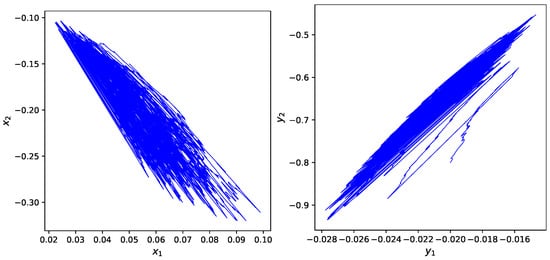
with $h_1(u)=h_2(u)=1.2cos(u)$ and $g_1(u)=g_2(u)=1.2cos(u)$. ${\varrho }_1(u)={\varrho }_2(u)=0.4u$ and ${\overline{\varrho }}_1(u)={\overline{\varrho }}_2(u)=0.2u$. As a result, system (33) has a chaotic attractor with initial condition $x_1(0)=0.05$, $x_2(0)=-0.15$, $y_1(0)=-0.02$, $y_2(0)=-0.8$, as shown in Figure 2.

Figure 2. The chaotic attractor of the system (33).

The corresponding response system of (35) is given as

$$\left\{\begin{array}{cc}\hfill d{\tilde{x}}_i(t)=& [-a_i{\tilde{x}}_i(t)+\sum _{j=1}^2{b}_{ij}{h}_j({\tilde{y}}_j(t))+\underset{j=1}{\overset{2}{\bigwedge }}{T}_{ij}{\nu }_j+\underset{j=1}{\overset{2}{\bigwedge }}{\alpha }_{ij}{h}_j({\tilde{y}}_j(t))\hfill \\ \hfill & +\underset{j=1}{\overset{2}{\bigvee }}{S}_{ij}{\nu }_j+\underset{j=1}{\overset{2}{\bigvee }}{\beta }_{ij}{h}_j({\tilde{y}}_j(t))+I_i+u_i(t)]dt+{\varrho }_i(t,{\tilde{x}}_i(t))d\omega (t),t\ne t_{\tau },\hfill \\ \hfill d{\tilde{y}}_j(t)=& [-{\overline{a}}_j{\tilde{y}}_j(t)+\sum _{i=1}^2{\overline{b}}_{ji}{g}_i({\tilde{x}}_i(t))+\underset{i=1}{\overset{2}{\bigwedge }}{T}_{ji}{\overline{\nu }}_i+\underset{i=1}{\overset{2}{\bigwedge }}{\overline{\alpha }}_{ji}{g}_i({\tilde{x}}_i(t))\hfill \\ \hfill & +\underset{i=1}{\overset{2}{\bigvee }}{S}_{ji}{\overline{\nu }}_i+\underset{i=1}{\overset{2}{\bigvee }}{\overline{\beta }}_{ji}{g}_i({\tilde{x}}_i(t))+J_j+v_j(t)]dt+{\overline{\varrho }}_j(t,{\tilde{y}}_j(t))d\omega (t),t\ne t_{\tau },\hfill \\ \hfill \Delta {\tilde{x}}_i(t_{\tau })& ={\tilde{x}}_i(t_{\tau }^{+})-{\tilde{x}}_i(t_{\tau }^{-})=({\xi }_i-1){\tilde{x}}_i(t_{\tau }),\hfill \\ \hfill \Delta {\tilde{y}}_j(t_{\tau })& ={\tilde{y}}_j(t_{\tau }^{+})-{\tilde{y}}_j(t_{\tau }^{-})=({\zeta }_j-1){\tilde{y}}_j(t_{\tau }),\hfill \end{array}\right.$$

(34)

where $a_i,{\overline{a}}_j,b_{ij},{\overline{b}}_{ji},{\alpha }_{ij},{\overline{\alpha }}_{ji},{\beta }_{ij},{\overline{\beta }}_{ji},T_{ij}$, $S_{ij},{\nu }_j,{\overline{\nu }}_i$ for $i\in {\mathcal{I}}_1\triangleq \{1,2\},j\in {\mathcal{J}}_1\triangleq \{1,2\}$ are provided in system (33). It is not difficult to check that $k_1={max}_{i\in {\mathcal{I}}_1}\{r_i\}=-8.84$, $k_2={max}_{j\in {\mathcal{J}}_1}\{s_j\}=-8.824$, $k=\frac{T_c}{T_0}max\{k_1,k_2\}=-6.5211$, $L_j^h=L_i^g=1.2$, ${\eta }_i={\overline{\eta }}_j=1$ for $i\in {\mathcal{I}}_1,j\in {\mathcal{J}}_1$. By choosing PDT as $T_c=1.85$, then the Assumption 1, Assumption 2 and condition $k<min\{\psi ,\phi ,-\frac{T_c}{T_0}\frac{ln\zeta }{{\nu }_{\tau }}\}$ $=min\{2.6,1.7148,-5.7945\}$ in Theorem 1 are satisfied with ${\theta }_1={\theta }_2=1.3$, ${\vartheta }_1={\vartheta }_2=1.8$, ${ϵ}_1={ϵ}_2=1.3$, ${\varsigma }_1={\varsigma }_2=1.6$, $p=0.3$ and $q=1.9$. Therefore, according to Theorem 1, the drive–response systems (33) and (34) have a synchronized within PDT $T_c=1.85$ which is less than $T_0=2.5033$ and $T_1=2.0305$ under controller (7), where $T_1$ is the ST estimation for FXT synchronization, as provided in Equation (6). The results are shown in Figure 3.

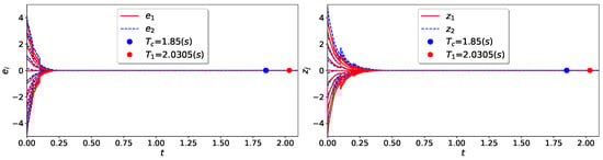
Figure 3. Evaluation of synchronization errors for Example 1.

Example 2.

For $n=m=3$, consider the following impulsive fuzzy BAMNNs with stochastic perturbations

$$\left\{\begin{array}{cc}\hfill d{x}_i(t)=& [-a_i{x}_i(t)+\sum _{j=1}^3{b}_{ij}{h}_j(y_j(t))+\underset{j=1}{\overset{3}{\bigwedge }}{T}_{ij}{\nu }_j+\underset{j=1}{\overset{3}{\bigwedge }}{\alpha }_{ij}{h}_j(y_j(t))\hfill \\ \hfill & +\underset{j=1}{\overset{3}{\bigvee }}{S}_{ij}{\nu }_j+\underset{j=1}{\overset{3}{\bigvee }}{\beta }_{ij}{h}_j(y_j(t))+I_i]dt+{\varrho }_i(t,x_i(t))d\omega (t),t\ne t_{\tau },\hfill \\ \hfill d{y}_j(t)=& [-{\overline{a}}_j{y}_j(t)+\sum _{i=1}^3{\overline{b}}_{ji}{g}_i(x_i(t))+\underset{i=1}{\overset{3}{\bigwedge }}{T}_{ji}{\overline{\nu }}_i+\underset{i=1}{\overset{3}{\bigwedge }}{\overline{\alpha }}_{ji}{g}_i(x_i(t))\hfill \\ \hfill & +\underset{i=1}{\overset{3}{\bigvee }}{S}_{ji}{\overline{\nu }}_i+\underset{i=1}{\overset{3}{\bigvee }}{\overline{\beta }}_{ji}{g}_i(x_i(t))+J_j]dt+{\overline{\varrho }}_j(t,y_j(t))d\omega (t),t\ne t_{\tau },\hfill \\ \hfill \Delta x_i(t_{\tau })& =x_i(t_{\tau }^{+})-x_i(t_{\tau }^{-})=({\xi }_i-1)x_i(t_{\tau }),\hfill \\ \hfill \Delta y_j(t_{\tau })& =y_j(t_{\tau }^{+})-y_j(t_{\tau }^{-})=({\zeta }_j-1)y_j(t_{\tau }),\hfill \end{array}\right.$$

(35)

where $i\in \{1,2,3\},j\in \{1,2,3\}$, and the parameters of the system (35) are used as follows:

$$\{a_i\}=\left(\begin{array}{c}8.58\\ 7.384\\ 7.02\end{array}\right)\{{\overline{a}}_j\}=\left(\begin{array}{c}5.24\\ -4.52\\ 3.6\end{array}\right)\{b_{ij}\}=\left(\begin{array}{ccc}2.672& -2.656& 2\\ -2.74& 2& 2.624\\ -2& -2.74& -2.624\end{array}\right)$$

$$\{{\overline{b}}_{ji}\}=\left(\begin{array}{ccc}2.915& -3.1& 2.265\\ -2.86& -1.435& 2.725\\ -2.8& -2.46& -1.725\end{array}\right)\{{\alpha }_{ij}\}=\left(\begin{array}{ccc}-0.6& -0.6& -0.4\\ -0.6& -0.4& -0.2\\ -0.6& -0.2& -0.4\end{array}\right)$$

$$\{{\overline{\alpha }}_{ji}\}=\left(\begin{array}{ccc}-0.54& -0.46& -0.4\\ -0.78& -0.54& -0.45\\ -0.68& 0.48& -0.54\end{array}\right)\{{\beta }_{ij}\}=\left(\begin{array}{ccc}-0.6& -0.56& -0.4\\ -0.6& -0.6& -0.5\\ -0.6& -0.48& -0.54\end{array}\right)$$

$$\{{\overline{\beta }}_{ji}\}=\left(\begin{array}{ccc}-0.6& -0.26& -0.48\\ -0.4& -0.5& -0.6\\ -0.6& 0.52& -0.48\end{array}\right)\{I_i\}=\{J_j\}=\left(\begin{array}{c}0\\ 0\\ 0\end{array}\right)\{{\xi }_i\}=\{{\zeta }_j\}=\left(\begin{array}{c}0.58\\ 0.58\\ 0.58\end{array}\right)$$

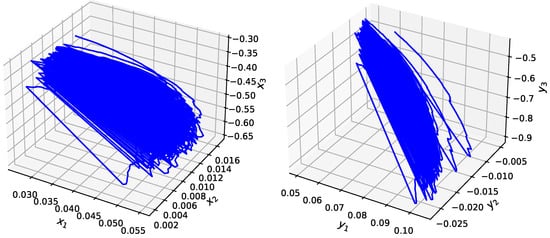
with $h_1(u)=h_2(u)=h_3(u)=1.2cos(u)$ and $g_1(u)=g_2(u)=g_3(u)=1.2cos(u)$. ${\varrho }_1(u)={\varrho }_2(u)={\varrho }_3(u)=0.2u$ and ${\overline{\varrho }}_1(u)={\overline{\varrho }}_2(u)={\overline{\varrho }}_3(u)=0.2u$. As a result, system (35) has a chaotic attractor with initial condition $x_1(0)=0.03$, $x_2(0)=-0.01$, $x_3(0)=-0.3$, $y_1(0)=0.06$, $y_2(0)=-0.005$ and $y_3(0)=-0.5$, as shown in Figure 4.

Figure 4. The chaotic attractor of the system (35).

The corresponding response system of (35) is given as

$$\left\{\begin{array}{cc}\hfill d{\tilde{x}}_i(t)=& [-a_i{\tilde{x}}_i(t)+\sum _{j=1}^m{b}_{ij}{h}_j({\tilde{y}}_j(t))+\underset{j=1}{\overset{m}{\bigwedge }}{T}_{ij}{\nu }_j+\underset{j=1}{\overset{m}{\bigwedge }}{\alpha }_{ij}{h}_j({\tilde{y}}_j(t))\hfill \\ \hfill & +\underset{j=1}{\overset{m}{\bigvee }}{S}_{ij}{\nu }_j+\underset{j=1}{\overset{m}{\bigvee }}{\beta }_{ij}{h}_j({\tilde{y}}_j(t))+I_i+u_i(t)]dt+{\varrho }_i(t,{\tilde{x}}_i(t))d\omega (t),t\ne t_{\tau },\hfill \\ \hfill d{\tilde{y}}_j(t)=& [-{\overline{a}}_j{\tilde{y}}_j(t)+\sum _{i=1}^n{\overline{b}}_{ji}{g}_i({\tilde{x}}_i(t))+\underset{i=1}{\overset{n}{\bigwedge }}{T}_{ji}{\overline{\nu }}_i+\underset{i=1}{\overset{n}{\bigwedge }}{\overline{\alpha }}_{ji}{g}_i({\tilde{x}}_i(t))\hfill \\ \hfill & +\underset{i=1}{\overset{n}{\bigvee }}{S}_{ji}{\overline{\nu }}_i+\underset{i=1}{\overset{n}{\bigvee }}{\overline{\beta }}_{ji}{g}_i({\tilde{x}}_i(t))+J_j+v_j(t)]dt+{\overline{\varrho }}_j(t,{\tilde{y}}_j(t))d\omega (t),t\ne t_{\tau },\hfill \\ \hfill \Delta {\tilde{x}}_i(t_{\tau })& ={\tilde{x}}_i(t_{\tau }^{+})-{\tilde{x}}_i(t_{\tau }^{-})=({\xi }_i-1){\tilde{x}}_i(t_{\tau }),\hfill \\ \hfill \Delta {\tilde{y}}_j(t_{\tau })& ={\tilde{y}}_j(t_{\tau }^{+})-{\tilde{y}}_j(t_{\tau }^{-})=({\zeta }_j-1){\tilde{y}}_j(t_{\tau }),\hfill \end{array}\right.$$

(36)

where $a_i,{\overline{a}}_j,b_{ij},{\overline{b}}_{ji},{\alpha }_{ij},{\overline{\alpha }}_{ji},{\beta }_{ij},{\overline{\beta }}_{ji},T_{ij}$, $S_{ij},{\nu }_j,{\overline{\nu }}_i$ for $i\in {\mathcal{I}}_2\triangleq \{1,2,3\},j\in {\mathcal{J}}_2\triangleq \{1,2,3\}$ are provided in system (35). It is not difficult to verify that $k_1={max}_{i\in {\mathcal{I}}_2}\{r_i\}=16.5292$, $k_2={max}_{j\in {\mathcal{J}}_2}\{s_j\}=15.7776$, $k=\frac{T_c}{T_0}max\{k_1,k_2\}=8.1882$, $L_j^h=L_i^g=1.2$, ${\eta }_i={\overline{\eta }}_j=0.1$ for $i\in {\mathcal{I}}_2,j\in {\mathcal{J}}_2$. By choosing PDT as $T_c=0.5$, then the Assumption 1, Assumption 2 and condition $k<min\{\psi ,\phi ,-\frac{T_c}{T_0}\frac{ln\zeta }{{\nu }_{\tau }}\}$ in Theorem 1 are satisfied with ${\theta }_1={\theta }_2={\theta }_3=4.2$, ${\vartheta }_1={\vartheta }_2={\vartheta }_3=6.3$, ${ϵ}_1={ϵ}_2={ϵ}_3=4.2$, ${\varsigma }_1={\varsigma }_2={\varsigma }_3=6.2$, $p=0.45$ and $q=1.45$. Therefore, according to Theorem 1, the drive–response systems (35) and (36) are synchronized PDT $T_c=0.5$ with less than $T_0=1.0093$ and $T_1=0.7758$ under controller (7), where $T_1$ is given by (6). The results are shown in Figure 5.

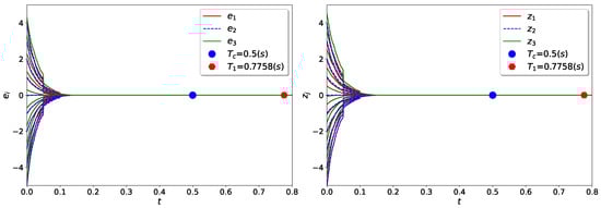
Figure 5. Evaluation of synchronization errors for Example 2.

Example 3.

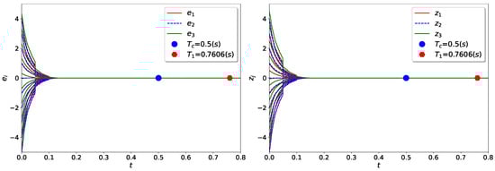
For $n=m=3$, consider the drive–response systems (35) and (36), given in Example 2, via controller (26). Here, $p_1=3$, $p_2=7$, $q_1=13$, and $q_2=9$, and the other parameters are the same as those given in Example 2. Thus, according to Theorem 2, the drive–response systems (35) and (36) have a synchronized PDT $T_c=0.5$ of less than ${\overline{T}}_0=0.9971$ and $T_1=0.7606$ under controller (26), as shown in Figure 6.

Figure 6. Evaluation of synchronization errors for Example 3.

Remark 4.

We performed three numerical simulations including two- and three-dimensional cases. The specific information is shown in Table 1. We can easily see that the ST estimations of the PDT synchronization can be preassigned according to the actual needs, and are, furthermore, more accurate than the ST estimations in previous works [19,20,21,33,40]. Two-dimensional and three-dimensional numerical simulations are disputed in Example 1 and Example 2, respectively, for the drive–response systems (1) and (2) under controller (7). In Example 2 and Example 3, we used different controllers (7) and (26), respectively, for drive–response systems (35) and (36). The difference between Example 2 and Example 3 is discussed in Remark 3.

Table 1. Comparison of examples.

Example	System	Dimension	Controller	${\mathit{T}}_{\mathit{c}}$	${\mathit{T}}_1$	${\mathit{\xi }}_{\mathit{i}}$	${\mathit{\zeta }}_{\mathit{j}}$
1	(33)	2	(7)	1.85	2.0305	0.48	1.48
2	(35)	3	(7)	0.5	0.7758	0.58	0.58
3	(35)	3	(26)	0.5	0.7606	0.58	0.58

Remark 5.

From the results of Examples 1, 2 and 3, we can see that the preassigned time $T_c$ is always less than the $T_0$ in Theorem 1 and ${\overline{T}}_0$ in Theorem 2. This implies that we are able to predefine the time of synchronization of the drive–response systems. Furthermore, the preassigned time $T_c$ is more accurate than the ST estimation $T_1$ introduced in Remark 1. From this view, compared to these previous works [19,20,21,33,40], the results in this paper are more applicable.

Remark 6.

From Figure 2 and Figure 4, we can see that the BAM neural network has hyper-chaotic attractors, and it also has good construction and higher associative memory capabilities. Because the higher chaotic properties of BAM neural networks can provide strong security, it can be employed in the field of image encryption and signal transmission.

5. Conclusions

In this paper, we investigated the PDT synchronization of impulsive fuzzy BAM neural networks with stochastic perturbations. First, we introduced some relevant results for PDT synchronization, fuzziness and stochastic neural networks. Then, based on these previous works, we combined impulse effect, fuzziness and stochastic perturbations for BAM neural networks. Next, a type of novel controller is designed for the considered system. After that, some sufficient conditions are obtained to ensure the PDT synchronization of the drive–response systems by using the Lyapunov function method. Finally, three numerical examples are provided to show the effectiveness of the obtained theoretical results of the proposed model. In future work, we may focus on the FXT/PDT synchronization of BAM neural networks with reaction–diffusion terms, as this area of research is important because of its practical applicability in certain fields [43,44].

References

- Kosko, B. Adaptive bi-directional associative memories. Appl. Opt. 1987, 26, 4947–4960. [Google Scholar] [CrossRef]
- Kosko, B. Bi-directional associative memories. IEEE Trans. Syst. Man. Cybern. 1988, 18, 49–60. [Google Scholar] [CrossRef]
- Hasan, S.M.R.; Siong, N.K. A VLSI BAM neural network chip for pattern recognition applications. In Proceedings of the ICNN’95—International Conference on Neural Networks, Perth, WA, Australia, 27 November–1 December 1995; pp. 164–168. [Google Scholar]
- Chau, F.T.; Cheung, B.; Tam, K.Y.; Li, L.K. Application of a bi-directional associative memory (BAM) network in computer assisted learning in chemistry. Computer Chem. 1994, 18, 359–362. [Google Scholar] [CrossRef]
- Wang, L.; Jiang, M.; Liu, R.; Tang, X. Comparison BAM and discrete Hopfield networks with CPN for processing of noisy data. In Proceedings of the 2008 9th International Conference on Signal Processing, Beijing, China, 26–29 October 2008; pp. 1708–1711. [Google Scholar]
- Wang, W.; Wang, X.; Luo, X. Finit-time projective synchronization of memristor-based BAM neural networks and applications in image encryption. IEEE Access 2018, 6, 56457–56476. [Google Scholar] [CrossRef]
- Konnur, R. Synchronization-based approach for estimating all model parameters of chaotic systems. Phy. Rev. E. 2003, 67, 027204. [Google Scholar] [CrossRef]
- Rakkiyappan, R.; Latha, V.P.; Zhu, Q.; Yao, Z. Exponential synchronization of Markovian jumping chaotic neural networks with sampled-data and saturating actuators. Nonlinear Anal. Hybrid Syst. 2017, 24, 28–44. [Google Scholar] [CrossRef]
- Cao, J. Global asymptotic stability of delayed bi-directional associative memory. Appl. Math. Comput. 2003, 142, 333–339. [Google Scholar]
- Mathiyalagan, K.; Park, J.H.; Sakthivel, R. Synchronization for delayed memristive BAM neural networks using impulsive control with random nonlinearities. Appl. Math. Comput. 2015, 259, 967–979. [Google Scholar] [CrossRef]
- Sader, M.; Abdurahman, A.; Jiang, H.J. General decay synchronization of delayed BAM neural networks via nonlinear feedback control. Appl. Math. and Comput. 2018, 337, 302–314. [Google Scholar] [CrossRef]
- Hong, Y.; Huang, J. Finite-time control for robot manipulators. Syst. Control Lett. 2002, 46, 243–253. [Google Scholar] [CrossRef]
- Bhat, S.P.; Bernstein, D.S. Finite-time stability of homogeneous systems. In Proceedings of the American Control Conference, Albuquerque, NM, USA, 6 June 1997; Volume 4, pp. 2513–2514. [Google Scholar]
- Jiang, M.; Wang, S.; Mei, J.; Shen, Y. Finite-time synchronization control of a class of memristor-based recurrent neural networks. Neural Netw. 2014, 63, 133–140. [Google Scholar] [CrossRef] [PubMed]
- Velmurugan, G.; Rakkiyappan, R.; Cao, J. Finite-time synchronization of fractional-order memristor-based neural networks with time delays. Neural Netw. 2016, 73, 36–46. [Google Scholar] [CrossRef]
- Polyakov, A. Nonlinear feedback design for fixed-time stabilization of linear control systems. IEEE Trans. Autom. Control 2012, 57, 2106–2110. [Google Scholar] [CrossRef]
- Wan, Y.; Cao, J.; Wen, G. Robust fixed-time synchronization of delayed Cohen-Grossberg neural networks. Neural Netw. 2016, 73, 86–94. [Google Scholar] [PubMed]
- Hu, H.; Gao, B.; Xu, L. Finite-Time and Fixed-Time Attractiveness for Nonlinear Impulsive Systems. IEEE Tans. Autom. Control 2022, 67, 5586–5593. [Google Scholar] [CrossRef]
- Wang, Q.; Zhao, H.; Liu, A.; Li, L.; Niu, S.; Chen, C. Predefined-Time Synchronization of Stochastic Memristor-Based Bidirectional Associative Memory Neural Networks With Time-Varying Delays. IEEE Trans. Cogn. Devel. Sys. 2022, 14, 1584–1593. [Google Scholar] [CrossRef]
- You, J.; Abdurahman, A.; Sadik, H. Fixed/Predefined-Time synchronization of complex-valued stochastic BAM neural networks with stabilizing and destabilizing impulse. Mathematics 2022, 10, 4384. [Google Scholar] [CrossRef]
- Abudusaimaiti, M.; Abdurahman, A.; Jiang, H. Fixed/predefined-time synchronization of fuzzy neural networks with stochastic perturbations. Chaos Solitons Fractals 2022, 154, 111596. [Google Scholar] [CrossRef]
- Yang, T.; Yang, L.; Wu, C.; Chua, L. Fuzzy cellular neural networks: Theory. In Proceedings of the IEEE International Workshop on Cellular Neural Networks and Applications, Seville, Spain, 24–26 June 1996; pp. 181–186. [Google Scholar]
- Yang, T.; Yang, L.; Wu, C.; Chua, L. Fuzzy cellular neural networks: Applications. In Proceedings of the IEEE International Workshop on Cellular Neural Networks and Applications, Seville, Spain, 24–26 June 1996; pp. 225–230. [Google Scholar]
- Quteishat, A.; Lim, C.P.; Tan, K.S. A modified fuzzy min–max neural network with a genetic-algorithm-based rule extractor for pattern classification. IEEE trans. Syst. Man Cybern. 2010, 40, 641–650. [Google Scholar] [CrossRef]
- Kanakalakshmi, S.; Sakthivel, R.; Karthick, S.A.; Leelamani, A.; Parivallal, A. Finite-time decentralized event-triggering non-fragile control for fuzzy neural networks with cyber-attack and energy constraints. Eur. J. Control 2021, 57, 135–146. [Google Scholar] [CrossRef]
- Zhang, H.; Liu, J.; Ma, D.; Wang, Z. Data-core-based fuzzy min–max neural network for pattern classification. IEEE Trans. Neural Networks 2011, 2212, 2339–2352. [Google Scholar] [CrossRef] [PubMed]
- Kadak, U. Multivariate fuzzy neural network interpolation operators and applications to image processing. Expert Syst. Appl. 2022, 206, 117771. [Google Scholar]
- Li, S.; Hernández, M.A.B. Robust synchronization of chaotic systems with novel fuzzy rule-based controllers. Inform. Sci. 2019, 481, 604–615. [Google Scholar]
- Wang, P.; Li, X.; Wang, N.; Li, Y.; Shi, K.; Lu, J. Almost periodic synchronization of quaternion-valued fuzzy cellular neural networks with leakage delays. Fuzzy Sets Syst. 2022, 426, 46–65. [Google Scholar] [CrossRef]
- Gunasekaran, N.; Saravanakumar, R.; Joo, Y.; Kim, H. Finite-time synchronization of sampled-data T–S fuzzy complex dynamical networks subject to average dwell-time approach. Fuzzy Sets Syst. 2019, 374, 40–59. [Google Scholar]
- Duan, L.; Li, J. Fixed-time synchronization of fuzzy neutral-type BAM memristive inertial neural networks with proportional delays. Inform. Sci. 2021, 576, 522–541. [Google Scholar] [CrossRef]
- Li, X.; Song, S. Research on synchronization of chaotic delayed neural networks with stochastic perturbation using impulsive control method. Commun. Nonlinear Sci. Numer. Simulat. 2014, 19, 3892–3900. [Google Scholar] [CrossRef]
- Gu, H. Mean square exponential stability in high-order stochastic impulsive BAM neural networks with time-varying delays. Neurocomputing 2011, 74, 720–729. [Google Scholar] [CrossRef]
- Zhang, Y.; Li, L.; Peng, H.; Xiao, J.; Yang, Y.; Zheng, M.; Zhao, H. Finite-time synchronization for memristor-based BAM neural networks with stochastic perturbations and time-varying delays. Int. J. Robust Nonlinear Control 2018, 28, 5118–5139. [Google Scholar]
- Abdurahman, A.; Abudusaimaiti, M.; Jiang, H. Fixed/predefined-time lag synchronization of complex-valued BAM neural networks with stochastic perturbations. Appl. Math. Comp. 2023, 444, 127811. [Google Scholar]
- Lee, L.; Liu, Y.; Liang, J.; Cai, X. Finite time stability of nonlinear impulsive systems and its applications in sampled-data systems. ISA Trans. 2015, 57, 172–178. [Google Scholar] [PubMed]
- Yin, J.; Khoo, S.; Man, Z. Finite-time stability and instability of stochastic nonlinear systems. Automatica 2011, 47, 2671–2677. [Google Scholar]
- Zheng, M.; Li, L.; Peng, H.; Xiao, J.; Yang, Y.; Zhang, Y.; Zhao, H. Fixed-time synchronization of memristor-based fuzzy cellular neural network with time-varying delay. J. Franklin I. 2018, 355, 6780–6809. [Google Scholar] [CrossRef]
- Hardy, G.H.; Littlewood, J.E.; Polya, G. Inequalities; Cambridge University Press: Cambridge, UK, 1952. [Google Scholar]
- Kong, F.; Zhu, Q.; Sakthivel, R. Finite-time and fixed-time synchronization control of fuzzy cohen-grossberg neural networks. Fuzzy Sets Syst. 2020, 394, 87–109. [Google Scholar] [CrossRef]
- Cui, W.; Wang, Z.; Jin, W. Fixed-time synchronization of markovian jump fuzzy cellular neural networks with stochastic disturbance and time-varying delays. Fuzzy Sets Syst. 2021, 411, 68–84. [Google Scholar] [CrossRef]
- Higham, D.J. An algorithmic introduction to numerical simulation of stochastic differential equations. SIAM Rev. 2001, 43, 525–546. [Google Scholar]
- Bao, T.; Xu, Y. Global asymptotic stability of BAM neural networks with distributed delays and reaction–diffusion terms. Chaos Solitons Fractals 2006, 27, 134–1354. [Google Scholar]
- Hu, D.; Tan, J.; Shi, K.; Ding, K. Switching synchronization of reaction-diffusion neural networks with time-varying delays. Chaos Solitons Fractals 2022, 155, 111766. [Google Scholar]
Disclaimer/Publisher’s Note: The statements, opinions and data contained in all publications are solely those of the individual author(s) and contributor(s) and not of MDPI and/or the editor(s). MDPI and/or the editor(s) disclaim responsibility for any injury to people or property resulting from any ideas, methods, instructions or products referred to in the content. |
© 2023 by the authors. Licensee MDPI, Basel, Switzerland. This article is an open access article distributed under the terms and conditions of the Creative Commons Attribution (CC BY) license (https://creativecommons.org/licenses/by/4.0/).