Abstract
Line planning problems and differential pricing problems are complementary processes in the railway system, but these two problems were generally considered separate processes in most of the existing literature. This paper studies a time-dependent line planning problem and differential pricing problem with passenger train choice in high-speed railway networks under elastic origin-destination-period demand. After clearly and flexibly describing the organization cost of operators, the price cost, and the time cost of passengers in a physical infrastructure-based directed graph, a non-linear joint optimization model is designed with a diversity of optimization goals of maximizing the total revenue of railway operators minus the total travel cost of passengers. An algorithm based on a simulated annealing framework is designed to solve the joint optimization model, and six neighborhood search strategies are designed by combining the features of the studied problem and designed model closely to improve the efficiency of the solution search. The results based on both a toy railway network and a real-world railway network show that the optimized time-dependent line plan and differential price plan are beneficial to increasing the total revenue of railway operators and improving the travel service of railway passengers.
Keywords:
joint optimization; line planning; differential pricing; time-dependent elastic demand; simulated annealing MSC:
90-10; 90B06
1. Introduction
The high-speed railway (HSR) is becoming more and more popular and important in the passenger railway system because of its high speed, punctuality, comfort, and other advantages. In the HSR network, passengers pay close attention to pieces of information such as train routes, train arrival/departure time, and train prices when choosing trains [1,2]. The line planning problem (LPP) is the key link in the process of transforming passenger flow into train flow of transportation organization. It has become an important and difficult problem because of its practical significance, large scale, necessary combination with passenger train choice, and the basis for other planning processes in a railway system [3]. However, the LPP is largely directly affected by the pricing problem, which determines the revenue of railway operators and the travel choice of railway passengers.
The LPP is generally to determine a set of lines with their corresponding operation frequencies and stop plans [4]. Its optimization goals are usually to consider both railway operators and railway passengers, namely, to optimize the total costs of railway operators and to optimize the total travel costs of railway passengers. A line is actually a route served by trains in an HSR network, and a route specifies information such as the original station, destination station, and the sequence of visiting stations of serviced trains. The operation frequency of a route says how often service is provided along the route within a given time range (e.g., a day), namely, the number of operated trains. At the same time, the stop plan specifies the sequence of stopped stations of different operated trains along a route. Therefore, line planning highly influences the travel route, travel cost, and travel stop of passengers and highly determines the cost of operators. High-quality line planning can not only provide high-quality train services and reduce the total travel costs for passengers but also is of great significance for operators to reduce the total operating costs.
Revenue management has also been gradually applied in the passenger railway system to optimize the benefits for railway operators and passengers [5]. The differential pricing problem (DPP) is an important and complex strategy of revenue management applied in railway systems due to the multiple trains and multiple prices between the same OD pair. Specifically, it needs to implement differential pricing for different trains between the same OD pair, and these trains may have different stopping plans, different departure times, and different arrival times. There is a complex relationship between the LPP and the DPP. The line planning determines the operating costs of operators and the travel service level of passengers; however, the differential pricing determines the revenue of operators and the travel cost of passengers. Therefore, it is necessary to joint optimize the line planning problem and the differential pricing problem (LPP-DPP) from the perspective of operators and passengers for filling this research gap, which can not only make the line planning more effectively meet the passenger demand and increase the revenue of operators based on the consideration of differential pricing, but also make the differential pricing further influence the train operation choice and the passenger train choice.
In recent years, passengers have become increasingly concerned about train arrival/departure times in addition to train prices when they make train choices. Very few scholars had considered the LPP with train arrival/departure times under fixed time-dependent demand [1,6]. Additionally, the time-dependent line planning can determine the sketchy arrival/departure times of each operated train at each station stopped at by not only more reasonably describing the passenger train choice and better improving the passenger service level, but also helping the processing of the train timetabling and arranging the precise arrival/departure time of trains. However, passenger demand is an elastic change process with the price and train arrival/departure time, especially for the joint optimization of LPP-DPP, and passenger demand is recommended to be set to an elastic demand form.
In this paper, we develop a rigorous non-linear joint optimization model for LPP-DPP with passenger train choice in the HSR network under time-dependent elastic demand. The model is clearly described in a directed graph for maximizing the revenue of railway operators under the limitation of the total operating cost of railway operators and the total travel cost of passengers. The optimization process efficiently combines train operation choice with passenger train choice. The time-dependent elastic demand is assumed as an exponential function of the weighted average generalized travel cost of passengers. In order to solve the complex non-linear model, we design an efficient solving algorithm based on simulated annealing to deal with the joint optimization problem in a real-world case. This paper contributes to the literature as follows:
- A joint optimization model of the time-dependent line planning problem and differential pricing problem with passenger train choice in the HSR network under elastic demand is proposed.
- A directed graph is constructed to describe the passenger travel network that can efficiently combine the train operation choice and the passenger train choice, and an efficient solving algorithm is designed based on simulated annealing to solve the joint optimization model.
- A small toy network and a real-world case study are used to test the effectiveness and applicability of the joint optimization model.
The rest of this paper is organized as follows. Section 2 reviews the studies that are most relevant to this paper. Section 3 describes the joint optimization problem of line planning and differential pricing with time-dependent elastic demand on a directed graph, and proposes a non-linear joint optimization model with some constraints. Section 4 designs the solving algorithm based on simulated annealing. In Section 5, some numerical experiments on a small toy network and a China HSR network are presented to demonstrate the joint optimization method. Finally, the conclusion and further study are given in Section 6.
2. Literature Review
In this section, we review the line planning problems and the pricing problems related to this paper and summarize the literature gaps from our literature review.
2.1. Line Planning
The research on the line planning problem has been well studied and produced a lot of research results in the literature. Some scholars have carried out some reviews on the model optimization goals [3,7,8,9,10]. There are three main optimization goals of the problem: minimizing the total operating costs of trains from the perspective of the railway operators (cost-oriented), minimizing the total travel cost of passengers from the perspective of passengers (passenger-oriented), and minimizing both the total operating costs of trains and total travel cost of passengers (cost-and-passenger-oriented).
The cost-oriented models focus on minimizing the total operating costs of operators and providing service subject to the bottommost service and capacity requirements. These costs consist mainly of mileage-related costs [11], hourly-related costs [12], carriage-related costs [13], frequency-related costs [14], and total costs [15]. The passenger-oriented models aim to minimize the total travel costs of passengers subject to capacity constraints that maximize the direct travelers [16,17], minimize the travel times [18,19], and minimize the transfer times [20,21].
In addition, more and more scholars proposed cost-and-passenger-oriented models for minimizing both the costs of operators and passengers. Guan et al. [22] simultaneously optimized the train route configuration and passenger line assignment in a general transit railway network to construct the model cost-oriented and passenger-oriented to minimize the operating cost, passenger travel time, and line transfers. Borndörfer et al. [23] focused on finding lines and corresponding frequencies in public transportation and proposed a multicommodity flow model with the free route and dynamical line for considering both the operating costs of trains and the traveling time of passengers. Gallo et al. [24] presented four different models for the frequencies of a regional metro under the assumption of elastic demand and considered the costs of all transportation systems and the environmental costs. Canca et al. [25] optimized the line frequencies and capacities with passenger assignment in dense railway rapid transit networks to minimize operational costs and generalized user costs. Goerigk and Schmidt [4] determined the routes and the frequencies with user-optimal route choice in the long-distance rail network for minimizing the total passenger travel time of the passengers and total costs for the operator. Zhou et al. [26] integrated the line and the frequencies with passenger path assignment in urban rail transit networks to minimize the total operating cost, transfer penalty, and sum of in-vehicle and waiting time. Vermeir et al. [27] proposed a grid-based approach for the line planning problem and it can be integrated into many line planning algorithms. Furthermore, very few scholars considered the time information in the optimization of the line planning problem under time-dependent demand. Su et al. [6] and Zhao et al. [1] used this way of thinking to construct a cost-and-passenger-oriented model and design a simulated annealing algorithm to solve it. In addition, Canca et al. [28] considered a line planning problem for maximizing the net profit and used an adaptive large neighborhood search metaheuristic to solve it.
2.2. Revenue Management and Pricing
Revenue management has been widely used in many important traditional industry applications such as passenger air transport, air cargo, hotel, and car rental [29]. Armstrong and Meissner [30] gave an overview of the published research on the revenue management applied in the railway system. Differential pricing is an important strategy applied in the railway markets by revenue management, and it is based on the sensitivity of different passengers to the attributes of different train products in the same OD pair. Many countries use the differential pricing strategy in their railway markets, such as China, the United States, and the United Kingdom [5]. Many scholars have carried out fruitful research on the application of differential pricing in railway markets.
Vuuren [31] established a link between the economic theory of optimal pricing, price elasticities of demand, and marginal cost estimates for the Netherlands railway. Bharill and Rangaraj [32] studied a revenue management case in the Indian railway and suggested using differential pricing to increase revenue on average. Zheng and Liu [33] proposed a model to optimize the ticket price for one high-speed train and one fare grade in China. Qin et al. [34] constructed a differential pricing model under elastic demand with prospect theory and designed a simulated annealing algorithm to solve the model. Su et al. [35] presented the differential pricing model considering the time-dependent demand and passenger choice behaviors in intercity high-speed railway services and applied a simulated annealing algorithm to solve it. Qin et al. [36] combined the differential pricing with the stop plan for high-speed railways under elastic demand and designed a simulated annealing algorithm to solve it. In addition, many scholars pay attention to the joint optimization of pricing and seat allocation, and most of the pricing adopted differential pricing [5,37].
2.3. Literature Summary
Based on the literature review, abundant research results have been produced in the research of the line planning problem [1,4,6,22,23,24,25,26] and the pricing problem [2,5,33,34,35,36]. From our literature review, we have learned that the time-dependent line planning problem and the differential pricing problem were optimized separately. In order to better show the real-world railway systems and greatly meet the passenger demand, we propose a non-linear joint optimization model of time-dependent line planning and differential pricing in the HSR network. The model considers the time-dependent elastic demand and combines the train operation choice with the passenger train choice. Furthermore, it takes into account the characteristics of multiple trains, multiple stops, and multiple time periods. This paper proposes and solves the joint optimization problem of line planning and differential pricing integrating with the time information and the passenger train choice under time-dependent elastic demand in the HSR network. In Table 1, we show some of the literature in comparison with our problems and methods. It should be noted that only some of the literature with high relevance to this paper is presented here.

Table 1.
Comparison of relevant literature of different papers.
3. Problem Formulation
3.1. Notations and Assumptions
In this paper, the major notations are listed in Table 2.
Table 2.
Notations.
Then we summarize the main assumptions for the joint optimization of LPP-DPP with passenger train choice under time-dependent elastic demand.
Assumption 1.
A set of pre-determined candidate trains is given, and the joint optimization problem only select operation trains from it [23,26].
Assumption 2.
Elastic demand for a given OD pair in each time period decreases with the average generalized travel cost of passengers, which includes time and price cost [37].
Assumption 3.
Each time period has the same time for passengers entering a station, namely, the expected departure time of passengers. The dwell time of each train at each station is fixed and has nothing to do with the passengers getting on and off the train [1].
3.2. Passenger Travel Network
and denote the set of stations and the set of sections among the stations in a physical railway network. Based on historical data and space-time distribution of passenger demands on the network, a set of pre-determined candidate trains can be defined. For each candidate train , its origin station , destination station , capacity , and the sequence of visiting stations from the origin to the destination are pre-determined. In order to contract the choice of arrival/departure time for each candidate train, we define the departure time range for each candidate train from its origin station, where and are the earliest and latest departure times of the train. Moreover, is defined as the pure running time of train in the section , and as the consumed dwell time of train stopping at station . Note that and are only for calculating sketchy arrival/departure times of each operated train and for better matching of passenger demand, rather than for generating a feasible train timetabling.
Based on the considered physical railway network and candidate trains, a directed graph is constructed to describe the combination of train operation choice and passenger train choice. and denote the set of three types of nodes and the set of six types of directed arcs, respectively. Specifically, the three types of nodes are constructed for each candidate train at each visiting station , namely, the station nodes , arrival node , and departure node . Then, the sets of six types of directed arcs can be combined from these three types of nodes, namely, the set of boarding arcs , travel arcs , dwell arcs , transfer arcs , getting-off arcs , and virtual arcs .
Each boarding arc for train at station represents the behavior process of passengers getting on the train, its capacity is set as if and only if this train is selected to operate, namely, , and to stop at this station, namely, ; otherwise, it is 0. Each travel arc for train is for representing the behavior process of passengers traveling from the visiting station to the next visiting station . Its capacity is set as if the train is selected to operate; otherwise, it is 0. Each dwell arc for train at station is to represent the behavior process of passengers stopping at this station. Its capacity is set as if both the train is selected to operate and stop at this station; otherwise, it is 0. Each transfer arc from train to train at station represents the behavior process of passengers transferring from one train to another. Its capacity is set as when the two trains not only are selected to operate and stop at this station, but also satisfy the requirement of the minimum transfer time ; otherwise, it is 0. Each getting-off arc for train at station is represented by the behavior process of passengers getting off this train at this station. Its capacity is set as if both the train is selected to operate and stop at this station; otherwise, it is 0. In addition, each virtual arc from each station to each station for each OD pair is represented by the canceled travel of passengers from the origin station to the destination station, and it has no capacity restriction. Of course, only when passengers cannot use the above five types of arcs to complete the travel process will they choose the virtual arc, because the cost of choosing the virtual arc is set very high.
Figure 1 shows a toy physical railway network and three candidate trains, and Figure 2 shows the directed graph constructed based on Figure 1. By searching and determining the sequence of arcs in the directed graph, we can find the train route and passenger travel route.
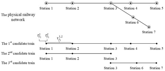
Figure 1.
A physical railway network and three candidate trains.
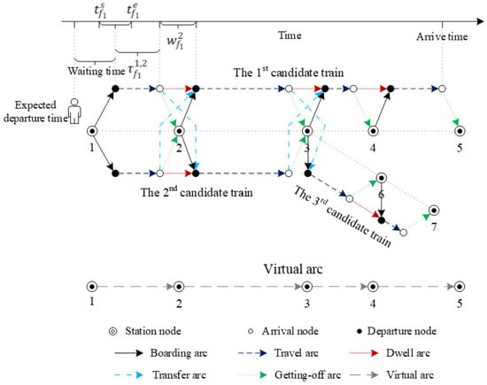
Figure 2.
The directed graph corresponding to Figure 1.
In addition, and denote two sets of arcs departing from and arriving at any type of node , and as any type of arc on the directed graph. It should be noted that the generation of nodes and arcs is related to the railway physical network and the candidate train, and has nothing to do with whether each candidate train is selected to operate and stop at specific stations. However, the availability of these arcs and their capacity depends on whether the candidate train is selected to operate and stop at the specific station. Therefore, the scale of a directed graph only depends on the size of the physical railway network and the number of candidate trains, but it is unrelated to the line plan.
3.3. Passenger Time-Dependent Elastic Demand
In order to reflect the elastic relationship between passenger demand and passenger travel service level, the elastic time-dependent demand is considered and given by a function of the weighted average generalized travel cost of passengers. Note that the passenger demand decreases with the generalized travel cost; this is the same as Hu et al. [5] and Deng et al. [37]. In this paper, the generalized travel cost of passengers considers the train price cost and travel time cost; it can more flexibly depict the price preference and travel time preference of passengers. Let us denote as a set of time periods for passengers entering their origin station , which is the expected departure time of passengers. Then, the passenger demand can be divided into many sets of origin-destination-period demands according to the time period of each OD pair. Next, we can use an elastic demand function to determine the elastic quantity for each origin-destination-period demand.
Passengers may pay differential prices for different trains between their origin station and their destination station, we denote the price for passengers traveling from their origin station to their destination station by train (CNY). In addition, the travel time cost of passengers is reflected in the difference between the time of arriving at the destination station and the expected departure time at the origin station, that is, the difference between the arrival time of the arrival node corresponding to the train at the destination station and the expected departure time of the corresponding time period. This includes the departure waiting time of passengers at the origin station, travel time in the passing section, and stop time through the stop station, as well as the transfer time at the visited transfer station. Additionally, denotes the transportation product provided by train for passengers corresponding to time period from their origin station to their destination station . Hence, the generalized travel cost of passengers on transportation product is formulated as:
where is a time cost parameter (CNY/minute). Then, the weighted average generalized travel cost of passengers in time period from to can be formulated as:
Now, we can construct the elastic demand function from the weighted average generalized travel cost of passengers, and we set the form of the function to be the exponential-linear demand function, which is similar to Hu et al. [5]. Thus, the elastic demand function is formulated as:
where is the total passenger demand for the OD pair in time period , is the total initial demand for the OD pair in time period corresponding to the initial weighted average generalized travel cost , and is the elasticity coefficient of the OD pair in time period .
3.4. Revenue and Cost Analysis
The revenue of railway operators and the cost of railway operators and passengers should be analyzed through each arc in a directed graph. We can define the cost for each arc and make the cost of the arc equal to the cost of the corresponding travel process. The revenue of the operators is considered the total price revenue minus the total operating cost, and the total cost of the passenger mainly considers the price cost and time cost during travel. denotes the number of passengers for the OD pair in time period on any type of arc , and the specific process of passenger demand allocation will be shown in a later subsection. Firstly, we analyze the total price revenue and the total operating cost of railway operators. The total price revenue can be determined as follows.
The total operating cost of railway operators consists of the total organization cost and the total train travel cost . The organization cost includes some fixed costs and the train travel cost includes some variable costs which are related to the engine time. Then, it can be formulated as follows:
where is the organization cost per train (CNY) and is a time cost parameter (CNY/minute). The total revenue of railway operators can be defined as the total price revenue minus the total operating cost, which can be expressed by the following equation:
Secondly, the total travel cost of passengers is specifically reflected in the arcs through which passengers complete their travel in a directed graph, so we need to analyze the costs of related arcs.
- (1)
- The price cost of each train for passengers is particularly reflected in the boarding arc and transfer arc, and their total price cost is the sum of the price of passengers at the origin station and transfer station, namely,
- (2)
- The total cost of waiting time for passengers CW at their origin station is shown on the boarding arc. It is the difference between the actual departure time and the expected departure time of passengers at the origin station.
- (3)
- The total cost of pure travel time of passengers CP from their origin station to their destination station is shown on the travel arc, it is the sum of the pure running time of all the train sections through which passengers complete their travel.
- (4)
- The total cost of dwell time of passengers CD at the station the train stopped at is shown on the dwell arc. It is the sum of the consumed time of all the stations the train stopped at through which passengers completed their travel.
- (5)
- The total cost of transfer time of passengers CH is shown on the transfer arc, it is the sum of the transfer time of all the transfer arcs for passengers who completed their transfer.
- (6)
- In the actual passenger demand distribution process in a directed graph, sometimes it happens that the passengers cannot complete their travel. We distribute this delayed passenger demand through the virtual arc, then the total delayed cost of the passengers can be calculated as follows:where is a fixed cost of each virtual arc, the value is set high.
Then, the total travel cost of passengers can be formulated as follows:
3.5. Model Formulation
The objective of the upcoming model is to maximize the total revenue of railway operators minus the total travel cost of passengers. That is,
where is a weight coefficient whose value locates in the range (0,1]. Its value affects the relationship between the total revenue of railway operators and the total travel cost of passengers in the optimization result.
Then, some constraints are considered in the model as follows:
- Train arrival/departure time constraint
Constraint (16) ensures that each operated train departs from its origin station within the time range , constraint (17) ensures its pure running time in each running section, and constraint (18) ensures its consumed dwell time at each stop station.
- Consistency constraint
Constraint (19) ensures that each operated train must stop at its origin station and destination station , and constraint (20) ensures that the number of the stop stations of the train cannot be more than , namely, the number of stations visiting by train.
- Price constraint
Constraint (21) is the consistency constraint of price and stop, which ensures that the price can be more than 0 only if train stops at stations and corresponding to the OD pair . Constraint (22) ensures that the price of the OD pair for train is bounded, where and are the lower and upper bounds, and the values of the bounds are subjected to the relevant policy. Constraint (23) ensures that the price between the OD pairs with long mileage is higher than that between the OD pairs with relatively short mileage.
- Flow balance constraint of passengers
These constraints can ensure the balanced allocation of passengers in a directed graph. For each total elastic demand , constraint (24) ensures that passengers depart from the station node with the connected boarding arcs or virtual arc, constraint (26) ensures that passengers finally arrive at the station node with the connected getting-off arcs or virtual arc, and constraint (25) ensures that the number of passengers entering an arrival node or leaving a departure node must be equal to the number of them leaving or entering the corresponding node.
- Validity constraint of visiting boarding arcs
Constraint (27) ensures that if the boarding arc allows passengers in time period to take train at their origin station , that is, , the number of passengers on the boarding arc can be more than 0. Constraint (28) ensures that the departure time of the corresponding train at the current station is later than the expected departure time of passengers, namely, the expected departure time of the corresponding time period .
- Capacity constraint
Constraint (29) ensures that passengers are allowed to get on and transfer into train along the corresponding boarding arc and transfer arc when the train stops at the current station and the capacity of the boarding arc and transfer arc are set as .
Constraint (30) ensures that passengers are allowed to travel by train along the corresponding travel arc when the train is selected to operate and the capacity of the travel arc is set as . Constraint (31) ensures that passengers are allowed to stop or pass along the corresponding dwell arc at the corresponding station when the train is selected to operate and the capacity of the dwell arc is set as .
Constraint (32) ensures that passengers are allowed to transfer from the train to along the corresponding transfer arc when the transfer arc is valid, that is, , and the capacity of the transfer arc is set as . Meanwhile, the valid variable of the transfer arc must be constrained by (33) and (34). Constraint (33) requires that both train and are selected to operate and stop at station , and constraint (34) requires that the transfer time for passengers satisfies the minimum transfer time , where is a very big non-negative integer.
Constraint (35) ensures that passengers are allowed to get off and transfer out to train along the corresponding getting-off arc and transfer arc when the train stops at the current station and the capacity of the getting-off arc and transfer arc are set as .
4. Solution Algorithm
The line planning problem is an NP-hard problem [1,11], and the joint optimization of the LPP-DPP is also very difficult to solve. Even if the joint optimization model can be approximately linearized, it will increase the number of variables and constraints very largely. The simulated annealing algorithm (SAA) of the heuristic approach is widely used in the LPP [1,38] and the DPP [35,36]. The SAA has a good application for this problem. In this paper, the joint optimization model will be solved under the framework of SAA.
4.1. SAA-Based Solution Algorithm Framework
The SAA-based solution algorithm framework for the joint optimization model is shown in Figure 3.
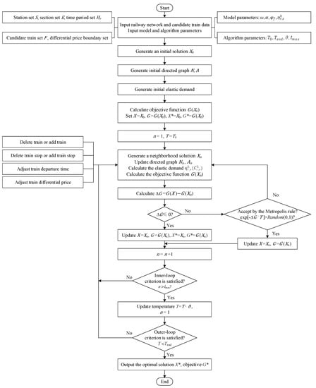
Figure 3.
SAA-based solution algorithm framework.
The solution algorithm is implemented by the following process, in which processes (4)–(6) will be repeated to continuously optimize the joint optimization model until the end condition is reached.
- (1)
- Candidate train set and differential price boundary generation: based on the physical railway network, and its current origin-destination-period demand and price level, generate a candidate train set and an upper-lower bound of the differential price between any serviceable OD pair for each candidate train;
- (2)
- Initial solution generation: select all the trains as the operated train from the candidate train set, set all the visiting stations as stopped stations of any train, and select a departure time for each operated train from the time range at its origin station; set the differential price of each operated train between any serviceable OD pair as the real price of the historical data. Based on the initial solution, initialize the directed graph;
- (3)
- Initial solution evaluation: calculate the weighted average generalized travel cost for each initial origin-destination-period demand based on the initial solution, and use the elastic demand function to obtain demand; based on the linear passenger flow allocation method, obtain the specific passenger flow on each arc in the directed graph, that is, obtain the passenger flow of each operated train in any operated section; calculate the objective function value of the initial solution based on the passenger flow allocation results and evaluate the initial solution;
- (4)
- Neighborhood searching procedure: search for a neighborhood solution of the current solution under neighborhood searching methods; update the directed graph based on the neighborhood solution;
- (5)
- Neighborhood solution evaluation: calculate the weighted average generalized travel cost for each origin-destination-period demand based on the current neighborhood solution, and use the elastic demand function to obtain each elastic origin-destination-period demand; based on the linear passenger flow allocation method, obtain the specific passenger flow on each arc in the directed graph; calculate the objective function value of the current neighborhood solution based on the passenger flow allocation results and evaluate the neighborhood solution;
- (6)
- Solution update: determine whether to accept the neighborhood solution based on the neighborhood solution evaluation;
- (7)
- End condition examination.
4.2. Initial Solution Generation
The algorithm selects the trains to operate from the candidate train set and obtains the optimized price from the price boundary, a set of candidate trains is generated based on the physical railway network and the space-time distribution of initial passenger demand, and then the operated train is selected from the candidate train set. The train set contains information about the origin station, destination station, sequence of visiting stations, and departure time range at the origin station of each candidate train. Based on the candidate train set, the upper and lower bounds of differential prices of each candidate train between any serviceable OD pair can be set. Then, we design the following method to generate the initial solution from the candidate train set and price boundary.
Step 0. Generate a set of train routes along any considered railway line in the physical railway network between any origin station and any destination station. Here, the origin and destination stations refer to any station capable of being the starting and ending station of trains, then get the information of origin station and destination station for each candidate train; set all the passing stations between the origin and destination station along each train route as visiting stations, then get the information of the sequence of visiting stations for each candidate train; specify a departure time range for each train route based on the space-time distribution of initial passenger demand, then get the information of departure time range at the origin station for each candidate train; set the capacity of each candidate train as ; generate the initial differential price set for each candidate train based on the candidate train set and real historical data; set the upper bound at 1.2 times the initial differential price of each candidate train between any OD pair and set the lower bound at 0.6 times the initial differential price of each candidate train between any OD pair;
Step 1. Set all trains in the candidate train set as operated trains, set all visiting stations of each train as stopped stations, set the lower bound of the departure time range of each candidate train as the departure time of the train at their origin station, and set the price for each candidate train between any serviceable OD pair as the actual current price;
Step 2. Based on the current line planning and differential pricing of Step 1, use the elastic demand function to calculate the elastic origin-destination-period demand, then use the linear passenger flow allocation method to obtain the passenger flow of each arc in the directed graph by the GUROBI solver;
Step 3. According to the sum of the number of passengers on boarding arcs, getting-off arcs, and transfer arcs of each train at each station stopped at, the station of each train whose sum of passengers is less than 50 is randomly set as the non-stopped station;
Step 4. Randomly set some stations stopped at among all stations stopped at of all operated trains as non-stopped-at stations and update the line planning; update the differential pricing by deleting all prices associated with the changing station; then generate the initial solution and set it as the current solution and best solution.
4.3. Neighborhood Searching Procedure
Based on the initial solution or current solution, the core part of the inner loop of the SAA is the construction of the neighborhood solution. Combined with the joint optimization of the LPP-DPP, we design six types of neighborhood search strategies, which are the delete train strategy, add train strategy, delete stopped station strategy, add stopped station strategy, adjust train departure time strategy, and adjust train price strategy. The adjustment process of the first four strategies related to the line planning will be accompanied by the adjustment of the differential pricing, and the adjustment process of the sixth strategy related to the differential pricing will be accompanied by the adjustment of the line planning, that is to say, the adjustment of the line planning and the differential pricing is a whole process.
4.3.1. Delete Train Strategy
The strategy is to select a random proportion of trains to delete from the operated train set of the current solution with a random probability according to the price revenue of trains. First, a random number is generated in the interval , where is the maximum delete ratio of all operated trains, which decreases gradually with the increase of the SAA iterations. Therefore, the actual number of deleted trains under the current strategy can be calculated as . Second, the price revenue of all operated trains in the current solution is calculated and sorted in order from small to large, which is denoted as the set . Select a certain percentage of trains from all the operated trains with zero revenue to stop running directly. Similarly, this percentage decreases with the increase in the number of iterations. The top trains in the set are selected as the set and the price revenue of the train number is denoted as . Third, calculate the probability that each train in the is selected to delete, and then select the deleted train by the roulette wheel selection method according to this probability. Fourth, based on the deleted trains, all prices associated with these trains are deleted to obtain the adjusted differential pricing.
4.3.2. Add Train Strategy
The strategy is to select some not operated trains to operate according to the average departure waiting time of passengers on all operating trains within each departure time period. First, a random number is generated in the interval , where is the maximum add ratio of all time periods ; therefore, the actual number of added time periods under the current strategy can be calculated as . Second, the average departure waiting time of corresponding trains in each departure time period in the current solution is calculated and sorted in order from small to large, which is denoted as set . The top time periods in set are selected as set and the average departure waiting time of the time period number is denoted as . Third, calculate the probability that each time period is selected to add trains, and then select the time period to add trains by the roulette wheel selection method according to this probability. Fourth, select a certain percentage of all the trains that are not operated in the selected time period to start to operate. If there are no trains that are not operated in the selected time period, select the trains that are not operated in the adjacent time period to carry out the same operation. Fifth, based on the added trains, set the train departure time as the middle value of the maximum neutral between the departure time of all operating trains in the current period, and set the price for each train between any serviceable OD pair as the actual current price, then obtain the adjusted differential pricing.
4.3.3. Delete Station Stopped at Strategy
The strategy is to select some of the stations stopped at by the all-operated trains to set as non-stopped-at stations with a certain probability, and it is based on the total price revenue at the station, the total number of passengers who get off and transfer out of the station, and the difference between the departure times of the first and last trains at the station corresponding to the current train. First, the value of all stations stopped at by the all-operated trains are calculated and recorded as set according to the order from small to large, then a random number is generated in the interval , where is the maximum delete ratio of the stations; therefore, the actual number of deleted stations under the current strategy can be calculated as . Second, select the top stations in set as set and record the value of the number station as . Third, calculate the probability that each station in the is selected to delete, and then select the deleted station by the roulette wheel selection method according to this probability. Fourth, based on the deleted station stopped at by each train, delete all prices associated with the changing station and obtain the adjusted differential pricing. In addition, if a train stops at a station without passengers getting on, getting off, or transferring, the station will be deleted directly.
4.3.4. Add Station Stopped at Strategy
The strategy is to select some non-stopped-at stations of the operated trains to be set as stations stopped at with a probability based on the average price revenue of other trains that stopped at the station, the average number of passengers who get off and transfer out of the station of other trains that stopped at the station, and the difference between the departure times of the first and last trains that stopped at the station corresponding to the current train. First, the value of all non-stopped-at stations of the all-operated trains is calculated and recorded as set according to the order from small to large, then a random number is generated in the interval , where is the maximum delete ratio of the stations; therefore, the actual number of deleted stations under the current strategy can be calculated as . Second, select the top stations in set as set and record the value of the number station as . Third, calculate the probability that each station in is selected to add, and then select the added station by the roulette wheel selection method according to this probability. Fourth, based on the added station stopped at of each train, set the prices associated with these changing stations to be the actual current prices and obtain the adjusted differential pricing.
4.3.5. Adjust Train Departure Time Strategy
The strategy is to select some trains from all operated trains to adjust the train departure time at the origin station according to the average waiting time of passengers with a random probability. First, a random number is generated in the interval , where is the maximum adjusted ratio of all operated trains, which decreases gradually with the increase in the SAA iterations. Therefore, the actual number of adjusted trains under the current strategy can be calculated as . Second, the average waiting time of each train in is calculated and sorted in order from small to large, which is denoted as . The top trains in set are selected as set and the average waiting time of train number is denoted as . Third, calculate the probability that each train in is selected to adjust, and then select the adjusted train by the roulette wheel selection method according to this probability. Fourth, the departure time of the selected trains at the origin station is uniformly subtracted from a fixed time, which decreases with the increase in the number of iterations.
4.3.6. Adjust Train Price Strategy
The strategy is to select some train prices for different trains serving the same OD pair to add or reduce prices according to the train price revenue between the OD pair. First, a random number is generated in the interval , where is the maximum adjusted ratio of all train prices between each OD pair, which decreases gradually with the increase of the SAA iterations. Therefore, the actual number of adjusted OD prices between each OD pair under the current strategy can be calculated as , here, is the number of total serviceable OD pairs of all operated trains. Second, the price revenue of each serviceable train of each OD pair is calculated and sorted in order from small to large, which is denoted as set . For each group of OD price revenue between each OD pair, the maximum value is denoted as . Third, calculate the probability that the train price for each train serving the OD pair in the is selected to adjust, and then select the adjusted OD price by the roulette wheel selection method according to this probability. Fourth, for a set of train OD prices between any OD pairs, when the probability is greater than a random number, add a fixed ticket value to the ticket price, when the probability is less than a random number, subtract a fixed ticket value from the ticket price.
4.4. Algorithm Step
The algorithm step of the proposed SAA-based solution method for solving the joint optimization of the LPP-DPP is described in Algorithm 1:
| Algorithm 1 Simulated Annealing Algorithm |
| Input: |
|
| Output: |
|
| Step 1: initial solution generation and evaluation |
|
| Step 2: neighborhood searching and evaluation |
|
| Step 3: update the current solution and the best solution |
|
| Step 4: check the end condition of the inner loop |
|
| Step 5: check the end condition of the outer loop |
|
5. Numerical Experiments
In this section, a toy railway network and a real-world railway network are used to verify the effectiveness of the joint optimization model of the LPP-DPP and the solving efficiency of the SAA-based algorithm. We carry out sensitivity analysis using small-scale experiments based on the toy network, then carry out some experiments based on the real-world railway network. The numerical experiments are conducted using MATLAB R2019b, GUROBI optimizer version 10.0.0, and the YALMIP toolbox. The small case is run on a personal computer with an Intel Core i5-12400 2.50 GHz CPU and 16GB RAM, and the real-world case is run on a workstation equipped with an Intel Xeon W-2145 3.70 GHz CPU and 128GB RAM, it is a Dell-branded device purchased by an individual and placed in his personal office in Changsha, China.
5.1. A Small Case Study
The small-scale toy railway network is the same as the network in Figure 1. It consists of two lines, seven stations, and six sections, and the pure running time of each train is marked in Figure 4. The first line consists of stations 1, 2, 3, 4, and 5, the second line consists of stations 3, 6, and 7, and the two lines share station 3. The sequence of visiting stations, the sequence of the initially stopped stations, and the departure time range at the origin station (minute) of candidate trains are given in Table 3. The initial differential price, price lower bound, and price upper bound of each candidate train are generated by the price between the OD pairs in Table 4, that is, the initial price between the OD pairs of each candidate train is the same. The initial origin-destination-period demand of each OD pair in each time period and the initial weighted average generalized travel cost of each OD pair in each time period for the elastic demand function are also given in Table 4.
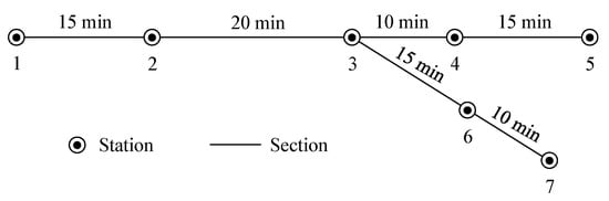
Figure 4.
Trains’ pure running times on the toy railway network.
Table 3.
The information of the candidate train.
Table 4.
The information of initial OD price and origin-destination-period demand.
In addition, the value of the weight coefficient is set at 0.8, the train capacity of each train is set at 600 seats/train-set, the organization cost of each train is set at 10,000/train-set, the stopping time of trains at each stopping station is set at 5 min, the minimum transfer time for passengers at the station is set at 30 min, the elasticity coefficient of each OD pair in each time period is set at 2, and the time cost parameters in the model are set at 0.5.
After 300 s of CPU time and 331 iterations, the convergence curve of the value of the objective function is shown in Figure 5, and the value of the objective function does not change after the 91st iteration. It can be seen from the figure that the value of the objective function converges from CNY 57,684.40 for the initial solution to CNY 112,024.60 for the final solution, and the increase of the final solution over the initial solution is 94.20%. Under the current algorithm framework, the case can converge to the final solution quickly, and the resulting final solution has a large improvement space compared with the initial solution. This shows that the algorithm has a high solving efficiency and can quickly find the final solution.
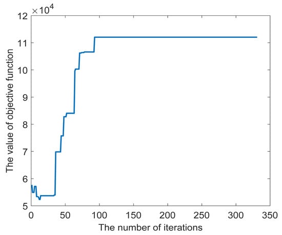
Figure 5.
The convergence curve of the small-scale case.
In this case, there are ten trains operating in the final solution. The sequence of stopped stations, departure time at the origin station, average load factor, and pure price revenue of each operated train are shown in Table 5. Compared with the initial solution, the number of stations stopped at of six operated trains is reduced by one or two, which indicates that the algorithm can effectively solve the optimal stations stopped at sequence of operated trains. From the departure time of each train at the origin station, the departure time of each train is relatively evenly distributed, which can effectively take into account the expected departure time needs of passengers. Three trains have an average load factor of more than 80%, two have an average load factor of more than 70%, and the rest have an average load factor of around 60%. In addition, from the perspective of the total price income of each operated train, each train can make a profit, which indicates that the model can effectively obtain the line plan and price plan beneficial to railway operators.
Table 5.
The information of all operated trains of the small-scale case.
Figure 6 shows the variation of passenger flow between the final solution and the initial solution of each OD pair in each period, and the X-axis is each OD pair and the Y-axis is the change value of each OD pair in each time period. It can be clearly seen from the figure that the increasing number of each OD for passenger flow in each period is more than the decreased number, which indicates that the elastic demand function can effectively regulate passenger flow. When the passenger travel cost is higher than the initial cost, the passenger flow decreases, and when the passenger travel cost is lower than the initial cost, the passenger flow increases, indicating that the model can fully take into account the passenger travel cost. Therefore, the model can effectively take into account various considerations in the objective, that is, it can effectively take into account the objectives of both railway operators and passengers.
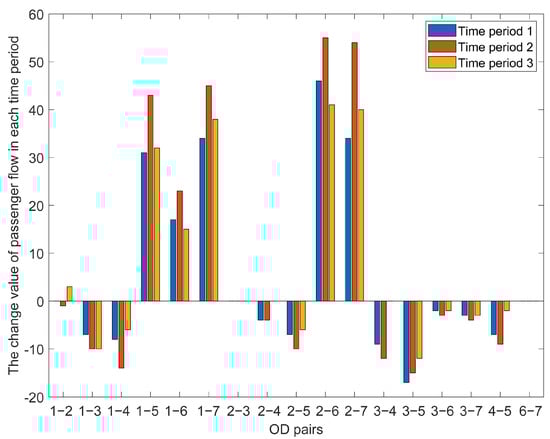
Figure 6.
The change value of each OD pair to passenger flow in each time period.
5.2. Sensitivity Analysis
It is necessary to perform sensitivity analysis for some key parameters and give some suitable values or ranges for setting these parameters. The analysis in this part is based on data from the small-scale case.
5.2.1. Impact Analysis of Weight Coefficient
The value of the weight coefficient affects the relationship between the total revenue of railway operators and the total travel cost of passengers in the optimization result. We fixed the other parameters and observed the change in the value of the objective function and the values of the above two parts in the final solution by changing the value of the weight coefficient. Figure 7 shows the changing trend of the value of the objective function when varies from 0.65 to 1 (interval: 0.05). The three curves in the figure show an overall upward trend. When is equal to 0.65, the value of the objective function is negative and the solution result of the model is abnormal. Therefore, in actual operation, the setting of the value of cannot be arbitrarily set to a small number between 0 and 1, for example, it cannot be set to less than 0.65 in the current case. When is equal to 1, the objective function is equal to the total revenue of railway operators, and the total travel cost of passengers is the highest. When the value of is after 0.7, the change range of total revenue of railway operators is not too large, while the total travel cost of passengers keeps rising. Therefore, in order to consider the interests of both operators and passengers, we suggest that the value of should be set around 0.8.
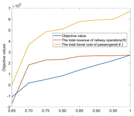
Figure 7.
Variation of the value of the objective function with .
5.2.2. Impact Analysis of Train Capacity
The passenger service capacity () of candidate trains determines the number of seats available for passengers. In Figure 8, we vary the value of the passenger service capacity from 400 to 1200 with a step of 100. When the train capacity varies between 400 and 800, the value of the objective function shows an increasing trend, and when the train capacity exceeds 800, the value of the objective function does not change. According to the trend of the curve, the increase in train capacity in a certain range (for example, less than 800) is conducive to the increase in the value of the objective function, but when the increase in train capacity exceeds a certain critical value (for example, higher than 800), the value of the objective function will not increase, because the change of train price is constrained by the price boundary.
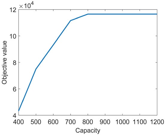
Figure 8.
Variation curve of the objective function with different passenger service capacities.
5.2.3. Impact Analysis of Price Boundary
The upper bound and lower bound of differential prices determine the range of price variation, thus determining price revenue and passenger cost. On the basis of the initial price, we increase the price to get the upper bound and reduce the price to get the lower bound, and the step size of the increase and decrease is 5% of the initial price. In Figure 9, with the increase in the variable range of price, the value of the objective function generally shows an upward trend. When the upper bound of the price is 105% to 130% of the initial price and the lower bound is 95% to 70% of the initial price, the rise of the objective function value is relatively obvious, and then the rise tends to moderate. In this case, when the upper bound of the price exceeds 130% of the initial price and the lower bound of the price is less than 70% of the initial price, continuing to expand the adjustment interval of the price does not significantly increase the value of the objective function. This is because the price cannot be increased blindly, and increasing the price means reducing the elastic demand. The two restrict each other to maintain the balance between operators and passengers.
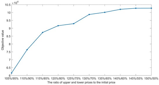
Figure 9.
Variation curve of the objective function with different upper and lower price bound.
5.3. A Real-World Case Study
As shown in Figure 10, a real-world railway network consists of 2 lines, 13 stations, and 12 sections. The first line runs from Beijing West Station to Zhengzhou East Station, the second line runs from Beijing West Station to Taiyuan South Station, and the two lines share five stations. The considered network includes the capital of Beijing and the provincial capitals of Taiyuan, Zhengzhou, and Shijiazhuang. In this paper, we only consider the single direction from Beijing West to Zhengzhou East and from Beijing West to Taiyuan South. The two stations Beijing West and Shijiazhuang can be used as the origin stations for trains, and the four stations Shijiazhuang, Taiyuan South, Handan East, and Zhengzhou East can be used as the destination stations for trains. We analyzed the real data statistics of the two lines by the China Railway ticketing system on 20 December 2016 (provided by the China Academy of Railway Sciences Co., Ltd.). The day from 6:00 to 21:00 will be divided into 5 time periods (e.g., from 6:00 to 8:59 is a time period), and the time-dependent demand includes 66 OD pairs and 48,579 initial passengers. Additionally, we pre-determined 61 candidate trains by combining the 2 lines with the demand.
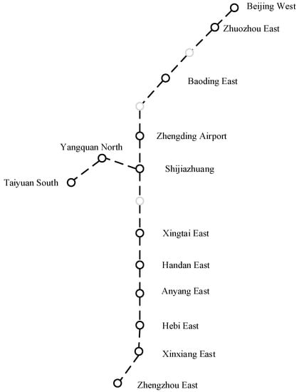
Figure 10.
Railway networks of Beijing–Zhengzhou HSR and Beijing–Taiyuan HSR.
In addition, the value of the weight coefficient is set at 0.8, the train capacity of each train is set at 1200 seats/train-set, the organization cost of each train is set at 30,000/train-set, the stopping time of trains at each stopping station is set at 5 min, the minimum transfer time for passengers at the station is set at 30 min, the elasticity coefficient of each OD pair in each time period is set at 1.5, and the time cost parameters in the model are set at 0.5.
In this case, the convergence curve of the value of the objective function is shown in Figure 11, and the value of the objective function converges after 5.16 h and 180 iterations. It can be seen from the figure that the value of the objective function converges from CNY 2,046,647.69 of the initial solution to CNY 2,686,000.60 of the final solution, and the increase in the final solution over the initial solution is 31.24%. It can be seen that the algorithm still has good adaptability to the current case and can get the final solution within an acceptable time range.
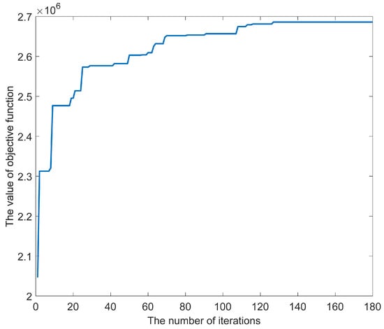
Figure 11.
The convergence curve of the real-world case.
The train diagram is shown in Figure 12. In the final solution, there are 30 trains in operation, among which 21 serve the first line and 9 serve the second line. Since we divide the passenger flow into five time periods, and the expected departure time of passengers within each time period is the same, it can be seen from the figure that the departure time of operated trains at the departure station are relatively concentrated on the expected departure time of passengers corresponding to these five time periods. Of course, if the time division unit is smaller, the departure time of the train at the origin station will be more widely concentrated around the expected departure time of the passengers at each time period. The average passenger load factor of each train in operation is shown in Table 6. The number of trains with an average load factor of more than 70% is 19, accounting for 63.33% of the total number of trains in operation. The total number of passengers getting on and getting off at each station and the number of stops at each station are shown in Figure 13. It can be seen from the figure that the line plan generated by the final solution can effectively match passenger demands. These show that the line plan obtained by the final solution can effectively meet the travel requirements of passengers and provide a high-quality line plan for railway operators.
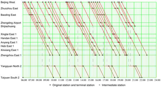
Figure 12.
Train diagram.
Table 6.
Distribution of average load factor for all operated trains.
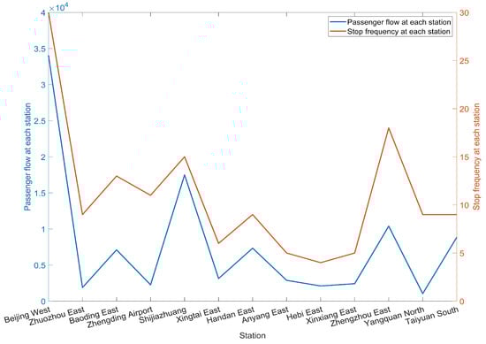
Figure 13.
The correlation between passenger demand and stop frequency at each station.
Figure 14 shows the change value of passenger flow in each time period. Under the regulation of the elastic demand function, the total number of passengers in the final solution is 50,486, which is 1907 people more than the initial solution. It can be clearly seen from the figure that most OD pairs increase the passenger flow in each period, which indicates that the line plan and price plan can serve passengers well. Of course, there are also a small number of OD pairs that reduce a lot of passenger flow in some periods, which is because these passengers cannot choose the right train in the final line plan and complete the travel, and the elastic demand function regulates these passengers. Based on the above analysis, we can conclude that the line plan and price plan in the final solution can effectively improve the income of railway operators and provide them with a high-quality line plan and differential price plan. Meanwhile, it can provide passengers with train products that meet the requirements of price and travel time at the same time.
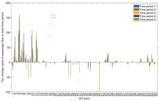
Figure 14.
The distribution of passenger numbers among all ODs and time periods.
6. Conclusions
In this study, we developed a non-linear joint optimization model for the time-dependent line planning problem and differential pricing problem (LPP-DPP) with passenger train choice in high-speed railway (HSR) networks under time-dependent elastic origin-destination-period demand. We described it based on a directed graph and solved it with an efficient algorithm. This algorithm is designed based on a simulated annealing framework combined with the existing linear commercial solver to complete the passenger flow allocation and objective function value calculation. We showed that the optimized time-dependent line plan and differential price plan can effectively increase the total revenue of railway operators and improve the travel level of railway passengers while providing both with higher quality line plans and more appropriate price plans, using a toy railway network and a real-world railway network of Beijing–Zhengzhou HSR and Beijing–Taiyuan HSR.
Future research can be further expanded in some possible ways. First, the scope of the problem can be further expanded, for example, the seat allocation decision can be introduced into the current decision-making, and the differential pricing decision of a single-class seat can be expanded to the differentiated pricing considering the levels of multiple seats. Second, although an effective SAA algorithm is designed in this study for a new joint optimization problem, more diversified solving methods can be used to solve the optimization model, such as the method of artificial intelligence and more efficient meta-heuristic algorithms, specifically, the method of artificial intelligence can be applied to various aspects such as HSR passenger demand estimation. Third, with the increase in research results, it is possible to compare the differences in solving methods in the background of similar problems.
Author Contributions
Conceptualization, W.Z.; methodology, W.Z.; software, X.L. and X.S.; validation, W.Z., X.L. and X.S.; formal analysis, X.L.; data curation, X.S.; writing—original draft preparation, X.L. and X.S.; writing—review and editing, W.Z., X.L. and X.S.; visualization, X.L. and X.S.; supervision, W.Z.; funding acquisition, W.Z. and X.L. All authors have read and agreed to the published version of the manuscript.
Funding
This research was funded by the National Natural Science Foundation of China, grant number 71871226, the general project of the Hunan Provincial Natural Science Foundation of China, grant number 2022JJ30057, the Hunan Provincial Innovation Foundation for Postgraduates, grant number CX20210234, and the Fundamental Research Funds for the Central Universities of Central South University, grant number 2021zzts0165.
Data Availability Statement
Not applicable.
Conflicts of Interest
The authors declare no conflict of interest.
References
- Zhao, S.; Wu, R.F.; Shi, F. A line planning approach for high-speed railway network with time-varying demand. Comput. Ind. Eng. 2021, 160, 107547. [Google Scholar] [CrossRef]
- Xu, G.M.; Zhong, L.H.; Hu, X.L.; Liu, W. Optimal pricing and seat allocation schemes in passenger railway systems. Transp. Res. Part E Logist. Transp. Rev. 2022, 157, 102580. [Google Scholar] [CrossRef]
- Schöbel, A. Line planning in public transportation: Models and methods. OR Spectr. 2012, 34, 491–510. [Google Scholar] [CrossRef]
- Goerigk, M.; Schmidt, M. Line planning with user-optimal route choice. Eur. J. Oper. Res. 2017, 259, 424–436. [Google Scholar] [CrossRef]
- Hu, X.L.; Shi, F.; Xu, G.M.; Qin, J. Joint optimization of pricing and seat allocation with multistage and discriminatory strategies in high-speed rail networks. Comput. Ind. Eng. 2020, 148, 106690. [Google Scholar] [CrossRef]
- Su, H.Y.; Tao, W.C.; Hu, X.L. A line planning approach for high-speed rail networks with time-dependent demand and capacity constraints. Math. Probl. Eng. 2019, 2019, 7509586. [Google Scholar] [CrossRef]
- Guihaire, V.; Hao, J.K. Transit network design and scheduling: A global review. Transp. Res. Part A Policy Pract. 2008, 42, 1251–1273. [Google Scholar] [CrossRef]
- Laporte, G.; Mesa, J.A.; Ortega, F.A.; Perea, F. Planning rapid transit networks. Socioecon. Plan. Sci. 2011, 45, 95–104. [Google Scholar] [CrossRef]
- Goerigk, M.; Schachtebeck, M.; Schöbel, A. Evaluating line concepts using travel times and robustness. Public Transp. 2013, 5, 267–284. [Google Scholar] [CrossRef]
- Laporte, G.; Mesa, J.A. The design of rapid transit network. In Location Science; Laporte, G., Nickel, S., Saldanha da Gama, F., Eds.; Springer: Cham, Switzerland, 2015; pp. 581–594. [Google Scholar]
- Claessens, M.T.; Van Dijk, N.M.; Zwaneveld, P.J. Cost optimal allocation of rail passenger lines. Eur. J. Oper. Res. 1998, 110, 474–489. [Google Scholar] [CrossRef]
- Goossens, J.W.; Van Hoesel, S.; Kroon, L. A branch-and-cut approach for solving railway line-planning problems. Transp. Sci. 2004, 38, 379–393. [Google Scholar] [CrossRef]
- Goossens, J.W.; Van Hoesel, S.; Kroon, L. On solving multi-type railway line planning problems. Eur. J. Oper. Res. 2006, 168, 403–424. [Google Scholar] [CrossRef]
- Torres, L.M.; Torres, R.; Borndörfer, R.; Pfetsch, M.E. Line Planning on Paths and Tree Networks with Applications to the Quito Trolebus System. In Proceedings of the 8th Workshop on Algorithmic Approaches for Transportation Modeling, Optimization, and Systems, Karlsruhe, Germany, 18 September 2008. [Google Scholar]
- Canca, D.; Andrade-Pineda, J.L.; De los Santos, A.; Calle, M. The Railway Rapid Transit frequency setting problem with speed-dependent operation costs. Transp. Res. Part B Methodol. 2018, 117, 494–519. [Google Scholar] [CrossRef]
- Bussieck, M.R.; Kreuzer, P.; Zimmermann, U.T. Optimal lines for railway systems. Eur. J. Oper. Res. 1996, 96, 54–63. [Google Scholar] [CrossRef]
- Yu, B.; Yang, Z.Z.; Jin, P.H.; Wu, S.H.; Yao, B.Z. Transit route network design-maximizing direct and transfer demand density. Transp. Res. Part C Emerg. Technol. 2012, 22, 58–75. [Google Scholar] [CrossRef]
- Schöbel, A.; Scholl, S. Line Planning with Minimal Traveling Time. In Proceedings of the 5th Workshop on Algorithmic Methods and Models for Optimization of Railways, Palma de Mallorca, Spain, 7 October 2005. [Google Scholar]
- Schmidt, M.; Schöbel, A. The complexity of integrating passenger routing decisions in public transportation models. Networks 2015, 65, 228–243. [Google Scholar] [CrossRef]
- Szeto, W.Y.; Wu, Y.Z. A simultaneous bus route design and frequency setting problem for Tin Shui Wai, Hong Kong. Eur. J. Oper. Res. 2011, 209, 141–155. [Google Scholar] [CrossRef]
- Szeto, W.Y.; Jiang, Y. Transit route and frequency design: Bi-level modeling and hybrid artificial bee colony algorithm approach. Transp. Res. Part B Methodol. 2014, 67, 235–263. [Google Scholar] [CrossRef]
- Guan, J.F.; Yang, H.; Wirasinghe, S.C. Simultaneous optimization of transit line configuration and passenger line transfer assignment. Transp. Res. Part B Methodol. 2006, 40, 885–902. [Google Scholar] [CrossRef]
- Borndörfer, R.; Grötschel, M.; Pfetsch, M.E. A column-generation approach to line planning in public transport. Transp. Sci. 2007, 41, 123–132. [Google Scholar] [CrossRef]
- Gallo, M.; Montella, B.; D’Acierno, L. The transit network design problem with elastic demand and internalisation of external costs: An application to rail frequency optimisation. Transp. Res. Part C Emerg. Technol. 2011, 19, 1276–1305. [Google Scholar] [CrossRef]
- Canca, D.; Barrena, E.; De-Los-Santos, A.; Andrade-Pineda, J.L. Setting lines frequency and capacity in dense railway rapid transit networks with simultaneous passenger assignment. Transp. Res. Part B Methodol. 2016, 93, 251–267. [Google Scholar] [CrossRef]
- Zhou, Y.; Yang, H.; Wang, Y.; Yan, X.D. Integrated line configuration and frequency determination with passenger path assignment in urban rail transit networks. Transp. Res. Part B Methodol. 2021, 145, 134–151. [Google Scholar] [CrossRef]
- Vermeir, E.; Durán-Micco, J.; Vansteenwegen, P. The grid based approach, a fast local evaluation technique for line planning. 4OR 2022, 20, 603–635. [Google Scholar] [CrossRef]
- Canca, D.; De-Los-Santos, A.; Laporte, G.; Mesa, J.A. Integrated railway rapid transit network design and line planning problem with maximum profit. Transp. Res. Part E Logist. Transp. Rev. 2019, 127, 1–30. [Google Scholar] [CrossRef]
- Klein, R.; Koch, S.; Steinhardt, C.; Strauss, A.K. A review of revenue management: Recent generalizations and advances in industry applications. Eur. J. Oper. Res. 2020, 284, 397–412. [Google Scholar] [CrossRef]
- Armstrong, A.; Meissner, J. Railway Revenue Management: Overview and Models; Working Paper; Lancaster University Management School: Lancaster, UK, 2020. [Google Scholar]
- Vuuren, D.V. Optimal pricing in railway passenger transport: Theory and practice in the netherlands. Transp. Policy 2002, 9, 95–106. [Google Scholar] [CrossRef]
- Bharill, R.; Rangaraj, N. Revenue management in railway operations: A study of the rajdhani express, indian railways. Transp. Res. Part A 2008, 42, 1195–1207. [Google Scholar] [CrossRef]
- Zheng, J.; Liu, J. The research on ticket fare optimization for China’s high-speed train. Math. Probl. Eng. 2016, 2016, 5073053. [Google Scholar] [CrossRef]
- Qin, J.; Qu, W.X.; Wu, X.K.; Zeng, Y.J. Differential pricing strategies of high speed railway based on prospect theory: An empirical study from China. Sustainability 2019, 11, 3804. [Google Scholar] [CrossRef]
- Su, H.Y.; Peng, S.T.; Deng, L.B.; Xu, W.X.; Zeng, Q.F. Optimal differential pricing for intercity high-speed railway services with time-dependent demand and passenger choice behaviors under capacity constraints. Math. Probl. Eng. 2021, 2021, 8420206. [Google Scholar] [CrossRef]
- Qin, J.; Li, X.Q.; Yang, K.; Xu, G.M. Joint Optimization of Ticket Pricing Strategy and Train Stop Plan for High-Speed Railway A Case Study. Mathematics 2022, 10, 1679. [Google Scholar] [CrossRef]
- Deng, L.B.; Xu, J.; Zeng, N.X.; Hu, X.L. Optimization Problem of Pricing and Seat Allocation Based on Bilevel Multifollower Programming in High-Speed Railway. J. Adv. Transp. 2021, 2021, 5316574. [Google Scholar] [CrossRef]
- Zhou, W.L.; Huang, Y.J.; Chai, N.J.; Li, B.; Li, X. A Line Planning Optimization Model for High-Speed Railway Network Merging Newly-Built Railway Lines. Mathematics 2022, 10, 3174. [Google Scholar] [CrossRef]
Disclaimer/Publisher’s Note: The statements, opinions and data contained in all publications are solely those of the individual author(s) and contributor(s) and not of MDPI and/or the editor(s). MDPI and/or the editor(s) disclaim responsibility for any injury to people or property resulting from any ideas, methods, instructions or products referred to in the content. |
© 2023 by the authors. Licensee MDPI, Basel, Switzerland. This article is an open access article distributed under the terms and conditions of the Creative Commons Attribution (CC BY) license (https://creativecommons.org/licenses/by/4.0/).