1. Introduction
Advances in computer and network technologies are completely transforming the world at an ever increasing speed. During the last three decades, financial exchanges went from an open outcry trading method to completely silent server rooms hosting complex global electronic trading systems. In the late 1990s, when information was already available in almost real time but trading floors were still full, the first studies using (what they believed to be) high-frequency data began to emerge. The authors of [
1] discuss the impact using high-frequency data would have on market microstructure research. Up until that time, data were collected only at points equally spaced in time (once a day, a week, a month, etc.), and all contemporaneous models were based on this assumption. With intraday data starting to become available for research, holistic data analysis was becoming challenging. Trades were no longer the sole source of information, since buy and sell quotes were recorded as well. Furthermore, consolidated market microstructure models could not properly explain the behavior of observed trading patterns, such as the ‘reflected-J’-shape (sometimes called a “U-shape”) that volume of orders, volatility of price, and bid–ask spread exhibit during the course of the trading day. The authors of [
2] review how the availability of high-frequency data is revolutionizing statistical models and the way we analyze data, as well as the computational and theoretical challenges that come with massive datasets. Using speed as a criterion, the author explains how technology changed electronic markets. He notes that market order executions that used to require more than 25 milliseconds to complete in 2001, were requiring less than 1 millisecond in 2010. During the same year (2010), there were up to 100,000 updates to bid and ask values per day, depending on the stock. The demand and supply characteristics of the limit order book are, as expected, of great importance to explain price dynamics, but its high dimensionality and complex evolution mechanics still prove to be difficult to model.
Technology not only allows for the possibility of updating trade and quote information within fractions of a second but also allows for companies to implement algorithmic trading (AT) techniques. These generally refer to either automatic trading strategies (deciding whether to enter or leave positions) or optimal order execution algorithms (liquidating large volume orders with as little market impact as possible), with little to no human interaction. The subset of traders that employ these techniques using high-speed systems is known as high-frequency traders. A thorough overview of the current research in high-frequency trading (HFT) is performed in [
3]. The studies are classified in five different categories (Financial Economic Research, Financial Theoretical Modeling Research, Order Book Dynamics Modeling Studies, Trading Strategies Studies, and HF Traders Behavioral Studies), with a comprehensive review in all of them. They find that, in general, HFT is seen with good eyes by both academia and the industry, providing liquidity and improving market quality. There are, however, problems when the market is under distress conditions, such as the May 2010 Flash Crash [
4]. This is mostly due to the automated nature of AT strategies, and the reasoning behind new regulation proposals on HFT. Furthermore, there is empirical evidence that HFT activity is concentrated in stocks from companies with a large capitalization (large-cap stocks) and these are the assets that impact the equity market indices the most. The authors of [
5] model the introduction of high-speed traders (machines) in a market populated only with slow traders (humans). Given their speed advantage, machines can shape the higher levels of the limit order book, and the authors conclude that, all other things being equal, there is a noticeable change in the transaction price distribution after they are introduced into the system. The authors of [
6] investigate the so-called HFT
arms race, with empirical evidence (25 Swedish large-cap stocks) that there is a significant difference between high-frequency traders with different latency profiles from a revenue perspective. Faster traders are not necessarily more accurate when analyzing new market information, but they do perceive more trading opportunities. It is important to mention, however, that the high-speed nature of HFT also allows for the rapid incorporation of fundamental values into current prices, thus enhancing market efficiency.
Finally, ref. [
7] calls for market microstructure research on the impact of HTF. Not only are the strategies employed by high-frequency traders different than the ones employed by low-frequency traders, but the latter also have to adapt their strategies for a market that contains high-frequency traders. The exchanges have also evolved, with new trading platforms, pricing models, and order priority rules. The paper ends by pointing to the important role of academia in policy research for this new market structure.
1.1. New Rules and Their Effects
Since the Financial Crisis of 2007–2008, and especially after the May 2010 Flash Crash, US regulatory commissions started developing new policies to try and avoid a repetition of such events. The authors of [
4] show that, although high-frequency traders did not start the May 2010 Flash Crash, they did cause a cascade effect, so many of these new regulations focus on HFT. One proposal from the Commodity Futures Trading Commission [
8] was planning to introduce control rules over all aspects of the trading cycle. Regulation Automated Trading (“Reg AT”), as it was known, defined automated trading very broadly and, had it been implemented, it would have affected almost all aspects of trading activity.
RegAT raised initial concerns in the industry, and its proposal was influential in the creation of the simulator used for this research [
9]. The truth is that nobody knows what is going to happen once these regulations are in place. The proposed rules may avoid new crashes, but they may also impair the proper functioning of the market. The authors of [
10] study mini flash crashes occurring during the six most volatile months in the U.S. equity market between 2006 and 2011. A mini flash crash is a crash happening during a time interval that is so small that it could be misrepresented as series of outlier price points in a low-frequency analysis. The authors of the study conclude that most of the mini flash crashes happen due to market fragmentation and the Regulation National Market System (Regulation NMS [
11]) only protecting the top of the LOB. In June 2020, CFTC withdrew RegAT from consideration and instead introduced “electronic trading principles” applicable to designated contract markets (DCMs. i.e., exchanges). The new rules, implemented 11 January 2021, task exchanges and trust them to implement appropriate rules that would mitigate market disruptions and system anomalies.
Most of the existing literature on the subject of rules and regulations falls under one of two categories. The research either analyzes the impact of implementing a policy in a particular exchange, months after the rule was put in place; or new market rules are proposed using a theoretical framework, with little empirical evidence of how such rules would work in practice.
An example of the regulation implemented without testing is targeting spoofing and attempts to stop it. The spoofing technique sends many small limit orders to the LOB, and quickly cancels them in sequence. The idea is to lead other high-speed algorithms (the only ones who can actually see the orders before they are canceled) to move in a pre-determined price direction. This is not the only reason why high-frequency traders submit batches of small orders, but it is one of the motivating factors behind proposing HFT regulations.
In September 2012, the Oslo Stock Exchange (OSE—Oslo Børs) implemented a new regulation setting a cost to the practice of
spoofing. Traders with a monthly order-to-trade ratio (OTR) in excess of 70 would have to pay a fee. OTR is the ratio of the number of orders submitted to the exchange divided by the number of these orders that are actually executed (traded). Using metrics such as the size of the bid–ask spread, realized volatility, and transaction costs, ref. [
12] conclude that there was no loss in market quality. Furthermore, the traders did not flee to other markets, and the only major effect of the new policy was that the average size of orders increased. In fact, no trader actually paid the fee by the day the study concluded, so the authors inferred that this regulation was a success.
In the above-mentioned regulation implemented in the Norwegian exchange, the OTR ignored orders that improved price, as well as the orders that stayed in the LOB for more than one second. In April 2012, similar regulation was implemented in Italy but, here, the OTR calculation was also including these orders. The ratio was also measured daily, instead of monthly. According to [
13], this implementation of the rule in the Borsa Italiana impacted market liquidity, unlike the Norwegian implementation. The authors of [
14] present a similar result, when a regulation targeting high-frequency traders in Canada led to less competition and a wider bid–ask spread, effectively raising transaction costs for low-frequency traders. The authors point to the fact that this result shows how critical the liquidity provided by high-frequency market makers is. The reason for highlighting these studies is to point out how important the details of the implementation are, and how crucial it is to experiment with such details before putting the rule in place.
A completely different route is to propose regulation based on a theoretical construct. We argue that, in this situation, it is even more important to empirically study the consequences of the implementation. Here, we mention the key paper [
15]. The authors propose a change to the way the Matching Engine operates in an exchange. The matching engine is the most essential component of a market exchange. It is responsible for managing the limit order book and matching orders to buy with orders to sell. The proposed “Frequent Batch Auctions” exchange, it is argued, would end the arms race that currently exists between high-frequency traders. We will discuss its implementation in details in
Section 1.2.
Before 2020, the Taiwanese Stock Exchange (TWSE) operated on a Frequent Batch Auction-type exchange model. The duration of each auction was random in an interval from
to
s. The end of day price was settled by a 5 min-long closing auction. On 23 March 2020, the TWSE changed the operation to continuous trading following a traditional continuous double auction model. Even though this was a FBA move in reverse, and concomitant to the COVID-19 pandemic emergence worldwide, it is worth looking at the conclusions drawn studying this event. First, ref. [
16] analyzed trading data using traditional regression models. They concluded that the move was beneficial for small cap stocks while large stocks were impacted in liquidity and price efficiency. The authors also concluded that foreign investors profited from the move, and, thus, foreign investment in the market increased. Therefore, they paint the switch as generally positive. In a subsequent paper, ref. [
17] cited the former research but they conducted their own study. They argue that the previous study “did not examine adverse selection and other market maker considerations” (on page 8 at the end of
Section 2 in [
17]). They also perform regressions and conclude, based on this adverse selection criteria, that the switch was largely negative in terms of market quality.
We are not singling out these papers to highlight the antiquated methods they use, or the fact that the significant finance literature glorifies regression as the tool of choice when operating with often-correlated observations. We are just pointing out that market studies can often be contradictory. Neither study has account level data, so their conclusions are solely inferred by analyzing trades and quotes.
1.2. Focus of This Paper
This paper builds on [
9], which presents SHIFT, with our attempt to extend the current agent-based modeling approach for financial markets. SHIFT is an order-driven, distributed asynchronous, and multi-asset financial market simulator. These characteristics, it is argued in our work, lead to more realistic simulations. Our objective with the SHIFT system was to create a laboratory environment for market microstructure research, equivalent in scientific rigor to traditional science fields. In such environments, experiments may be performed in realistic conditions but are isolated from other influencing factors.
We should mention other theoretical works comparing frequent batch auctions with continuous trading. The authors of [
18] model the interaction between slow and fast traders as a game of market selection, where each trader has to decide if they prefer to participate in a frequent batch auctions market or in a continuous double auctions market. They find that slow traders tend to be attracted to frequent batch auctions. They also derive that, even though fast traders demonstrate predatory behavior (chasing the slow traders to whichever market they decide to go to), slow traders are more protected from sniping and adverse selection in this type of market. The authors of [
19] design an experiment with human subjects to study the interaction with frequent batch auctions and continuous double auctions markets. The authors use a different type of market in each of the experiment sessions of their study, noise traders to generate liquidity, and a user interface where each subject would gather market information. They map the actions users perform to specific trader profiles (e.g., market maker, aggressive trader, etc.) and allow the “acquisition” of faster technologies to interact with the market. Based on this experiment, the authors conclude that frequent batch auctions lead to more liquidity, less predatory behavior, and less investment in technology.
Finally, we highlight [
20] as a study that employs an agent-based model to assess the optimal clearing interval in frequent batch auctions. The model, however, uses discrete time steps, as most agent-based models do. As discussed in [
9], we believe that real-time simulations with asynchronous interactions between the agents lead to more realistic results. For example, in the context of frequent batch auctions, an order submitted by a trader a few moments before the auction is performed may not arrive to the market exchange in time for the current auction and will be processed in the next. Another shortcoming of this model is that traders only trade in units of one.
The main objective of this work is to showcase an implementation of the frequent batch auctions, as close to reality as we believe possible in an academic environment. However, we are still in an academic environment (laboratory conditions), and, thus, there are limitations to the results we are presenting, some of which we discuss in this paper. Our goal is not to determine whether frequent batch auctions would or would not be a good substitute for continuous double auctions, but to point out the different market characteristics and expected behavior in case an exchange would decide to implement this matching mechanism in practice.
The rest of this paper is organized as follows.
Section 2 provides a brief description of the dynamics of frequent batch auctions, as compared to continuous double auctions.
Section 3 presents the results of our implementation of frequent batch auctions in SHIFT. We present comparisons between continuous double auctions and frequent batch auctions with different intervals in between auctions.
Section 4 concludes our paper, and presents future possible directions for our work.
2. Frequent Batch Auctions (FBA)
In this section, we present a brief explanation of how frequent batch auctions work. This is a summary of the work presented in [
15], where the authors propose the use of frequent batch auctions as a substitute to continuous double auctions, and [
21], in which the authors go into details on what a practical implementation of frequent batch auctions would entail. In our implementation using SHIFT, we closely follow these instructions. From this point on, we refer to frequent batch auctions as “FBAs” and to continuous double auctions as “CDAs”.
CDAs are the most common type of matching mechanism found in market exchanges today. Each asset has a limit order book (LOB) with two sides. One side of the LOB contains the current buy demand (bids) and one side contains the current sell supply (offers or asks). Traders can submit limit orders with the highest/lowest price they would be willing to buy/sell the respective asset. These orders will join the respective limit order book immediately upon arrival at the exchange. The limit order book follows a price-time priority. Specifically, orders with a better price or those that arrived first (if the same price) have priority in relation to the other existing orders in the book from an execution perspective. Traders may cancel their existing limit orders anytime they please. At any given moment in time, traders can also submit market buy or sell orders. These orders will be executed immediately, if possible, by matching the best available asks or bids at the time, following the limit order book price–time priority. Perhaps most importantly, in a CDA, the last traded prices and the current state of the limit order books are always available for any market participant to check.
It is also a common practice among market exchanges to host “call auctions” to determine the opening prices of traded assets. These call auctions, typically held before a market exchange opens, differ from CDA in that orders are not matched as they arrive, but accumulate in an order book up until a predetermined auction time, in what we will call the “order submission stage”. An order book example at the end of the order submission stage is presented in
Table 1. Here, we note that it is possible to have an intersection between the demand and supply volume, which is something that would never happen in CDAs.
When the order submission stage ends, the auction is carried out during what we will call the “auction stage”. The New York Stock Exchange (NYSE) calls this stage “Auction Freeze Period” and it happens when markets open or close with a duration of 1 min. During the auction stage, if there is an intersection between the demand and supply volumes, a price can be selected and all trades will happen at the selected price; otherwise, there is no price formation nor trades. The price is selected in such a way that maximizes the number of traded shares. To explain the process, in
Table 2, we summarize the orders received from
Table 1 and add extra columns. Demand indicates how many shares may be traded in the bid book if the respective price is the settled price. The supply column is similar but looks at the bid side of the LOB. The excess demand column simply calculates demand–supply. The price of USD
is chosen in this example since 600 shares can be traded at this price. At a price of USD
, only 500 shares would be traded.
If the bid volume at price level USD
was 400 instead of 300, this would have been the selected price because this price level would not only have maximized the number of traded shares (600) but it would also have the lowest absolute excess demand. If both of these rules are not enough to determine an unique price, it is common practice to select the price that is closer to the previous recorded price of the asset [
22].
All bids above the selected auction price and all asks below the selected auction price will be executed. The orders with prices equal to the selected auction price will only be fully executed in one side of the book (bids or asks). In the example above, 100 out of the the 200 shares in the ask orders at USD
will be matched with 100 shares among the 700 available in the other side of the book. The match is pro-rated. Specifically, assume that the 100 shares need to be matched with the 700 from the bid volume. We look at the existing bid orders that constitute that 700 shares volume. If there is only one order we are complete; we just execute 100 shares from that order. However, if there are, say, two orders, then we trade 50 shares with each order and the remaining shares are left for the next auction. The authors of [
15] did not specify if the pro-rate also takes into account the volume so, in our implementation, we simply divide the shares equally among the bid orders regardless of the order volume sizes. In the example, we use shares for ease of explanation. In the SHIFT implementation, 1 unit represents 100 shares. Thus, when pro-rating, we fill or partially fill orders in units of 100 shares.
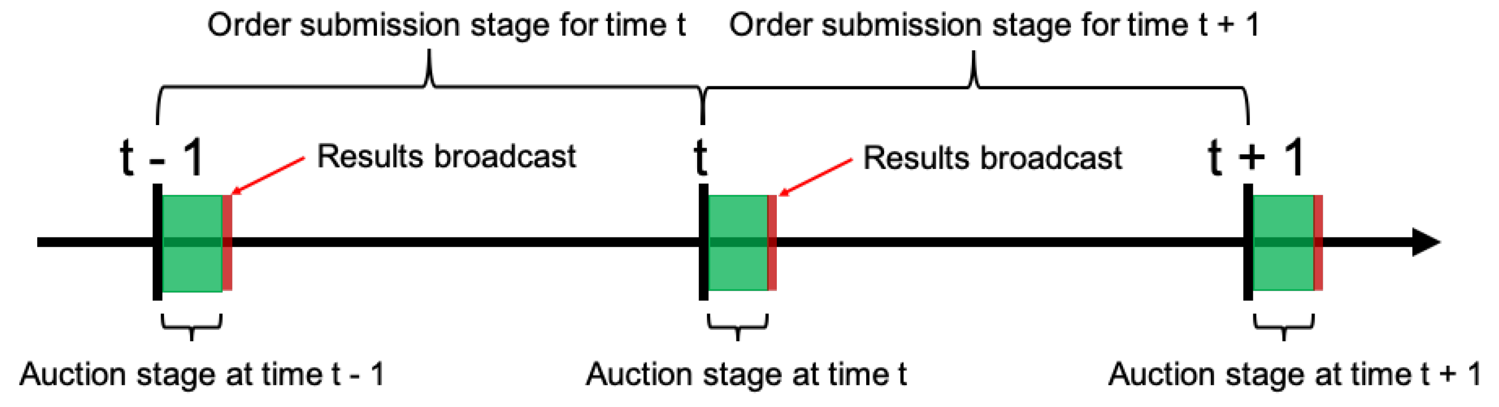
For CDAs, this auction stage happens before open and at close and sometimes one more outside trading hours. For example, as of 2022, NYSE has various pre-opening and opening auction sessions (details at
https://www.nyse.com/markets/nyse-arca/market-info accessed on 10 October 2022) every trading day. In contrast, for the frequent batch auctions (FBA), the entire trading period is composed of frequent call auctions. The process flow is displayed in
Figure 1, where the periods in green represent the processing time of the particular auction, and the periods in red represent the moment the results are broadcast to market participants. Note that the order submission stage restarts as soon as the auction processing begins. The orders are continuously accepted by the exchange, and the end of an order submission stage simply represents that no more orders will be accepted for that respective auction. During the order submission stage, the orders may be modified or cancelled.
The call action rules described above are all applicable in the FBA implementation. Additionally, orders remaining in the book from past auctions have precedence during the auction stage of subsequent auctions. This is the only time priority of the FBAs. In the practical implementation of FBAs, we devised a two step method to implement this. In the first step, we match shares with existing past auction shares at that level. If there are none, or if there are shares left to be matched after all prior action shares have been executed, we trade orders from the current auction in step two. In each of the steps, we pro-rate the orders as described above.
A very important feature of the FBA is that submitted orders (bid and asks) are sealed [
21]. The submitted orders are not communicated to participants during the order submission stage. This is the feature that is meant to prevent spoofing. At the end of the auction stage, the executed price and all the remaining orders in the order book are broadcasted to market participants, which is all the information they base their future actions on. If a particular order is not executed in a given auction, it will carry over to the subsequent auction, unless canceled by its owner. Sealing the orders also means there are no market orders in an FBA; all orders have to specify a price and a quantity.
2.1. A “Dark Pool-like” Implementation: HVCDA
In addition to the frequent batch auctions (FBAs) and continuous double auctions (CDA), we are going to implement a third market model that we call “Hidden Volume Continuous Double Auctions” (HVCDAs). In HVCDA, all the matching order rules are the same as in a CDA (same as the real market). The orders are matched with the same price–time priority, and outstanding limit orders stay in the order book until they are either matched with a market order or canceled. The difference is that all the market volume in HVCDAs is hidden from the market participants. Specifically, traders have no access to the limit order book. The only market feedback they have is the last traded price and any results from their own orders. This HVCDA implementation can be viewed as a proxy to the real world dynamics of dark pools. Dark pools do not release the volume and the only feedback market participants have is through reported trades and feedback to their own orders. However, the matching process in a dark pool is slightly different from our implementation as it is designed to earn the spread. This is the reason we do not call this implementation a dark pool; instead, we use the cumbersome acronym HVCDA.
An interesting observation is that the HVCDA implementation may be seen as a limit of the FBA exchange when the batch interval (order submission stage in
Figure 1) approaches zero.
2.2. Possible Shortcomings of Our Experiments
The objective of the proposed frequent batch auctions is to curb the arms race between the high-frequency traders. To become enticing to a well-functioning exchange, the auctions need to occur very frequently. The authors look at the normal processing times of market exchanges and suggest the interval in between auctions should be represented in a fraction of a second. We do not have the processing power of a real exchange, far from it. However, we use servers and a proper market design and, in our experiments with CDAs, market orders execute on average in 1 ms, while the auctions in the FBA format require 1–2 ms to process. The authors of the original FBA papers simulate the batch auctions based on a rate of messages seen during the flash crash (a reasonable worst case) and they find the auction stage occurs in under 10 milliseconds on a simple laptop.
However, despite the processing time being much better in our experiments using SHIFT, we observed that the system would start to struggle when the order submission stage interval was less than s long. Specifically, when using very short time intervals, messages between servers and clients would start to be lost and require FIX resend requests. We believe this happens due to the huge amount of messages that must be sent to all connected clients after the conclusion of each auction. In CDAs, every change in the order book can be broadcasted to clients as a differential. However, in FBAs, the final order book at the end of an auction will be completely different from the order book of the previous auction; thus, a differential is the same as rebroadcasting the entire order book. We mention this issue as a possible technology bridge that may need to be crossed to have the auctions in FBAs be more frequent than 500 milliseconds. This is a shortcoming of our experiments, since our tests cannot directly replicate the original intent of the proposers of FBAs. Nevertheless, as the reader will see in the following section, we experiment with different batch intervals in order to have an indication of the impact of the interval size on the results.
Another possible shortcoming of our experiments is the fact that we do not have specific trading strategies for CDA and FBA market-type participants. However, all traders in our experiments are noise traders, and noise traders would probably not change their behavior if FBAs were to be implemented in a real market exchange. Furthermore, one could argue that, if there was a change on the auction mechanism of a real exchange, most traders would likely not be prepared and adapt on day one, and our results can provide insights on that transition.
3. Experiments
In this section, we perform two sets of experiments. In the first experiment in
Section 3.1, we consider an endogenous market, where the information is limited to trades and limit order book data only. The idea is to consider a “normal” market–void from the effect of exogenous changes (e.g., news). In the second set of experiments (
Section 3.2), we consider market events that trigger sales orders that put the entire market under stress. We compare the resulting market statistics (price, return, limit order book, etc.) in both scenarios and compared depending on the market type: continuous double auction, FBA, and HVCDA.
For all experiments, we use zero intelligence agents to create the underlying market. These were constructed following the work performed in the Genoa Artificial Stock Market, described in [
23,
24], modified to work in a real-time environment. A description of the trading strategy they follow, as well as the results in the CDA market scenario, are presented in [
9]. We show in that work that the system successfully replicates all “stylized facts” of the observed equity movement in real exchanges. We use the results obtained as a baseline for comparison in
Section 3.1 and
Section 3.2.
Throughout our experiments, we implement two different types of markets: homogeneous or heterogeneous. This difference in agent behavior proved to have a very important effect to the severity of market stress produced [
9]. This classification is related to how we perform the initial wealth distribution among market participants. In both heterogeneous and homogeneous markets, traders are provided with the same total amount of buying and selling power. However, in the homogeneous markets, all the participants have similar amounts, while, in heterogeneous markets, we have a few traders (agents) with huge wealth and many traders with comparably little wealth. This is accomplished using a symmetric Dirichlet distribution for the initial wealth distribution, with different concentration parameter values that lead to either homogeneous or heterogeneous wealth values. The technical details of the process are described in [
9].
3.1. Experiment 1: Endogenous Market Scenarios
In our first set of experiments, there are 200 traders that constitute the market, and they collectively own 2,000,000 shares of Common Stock ticker (CS1), with an initial price USD . The traders also own an initial amount of cash equal to their initial amount of share holdings, so the total amount of capital in the market is USD 400,000,000. We determine the initial amount of shares using a symmetric Dirichlet distribution. The traders are assigned the share value in cash. The rest of the parameters in these experiments are as follows:
Simulation length M = 23,400 s ( h).
Each trader attempts to trade an average of either 390 or 780 times during the trading session, i.e., on average, they submit one limit order every minute or every half a minute, respectively, depending on the experiment.
Confidence level , i.e., the limit order size is uniformly distributed between and of the total buying or selling power of the traders, depending if it is a limit buy or a limit sell order, respectively. represents trading time j for the ith trader.
Homogeneous or heterogeneous wealth distribution. In homogeneous markets, traders have an approximately uniform distribution of initial wealth, with a low standard deviation. Heterogeneous markets are closer to what we see in reality, with a few large institutional investors.
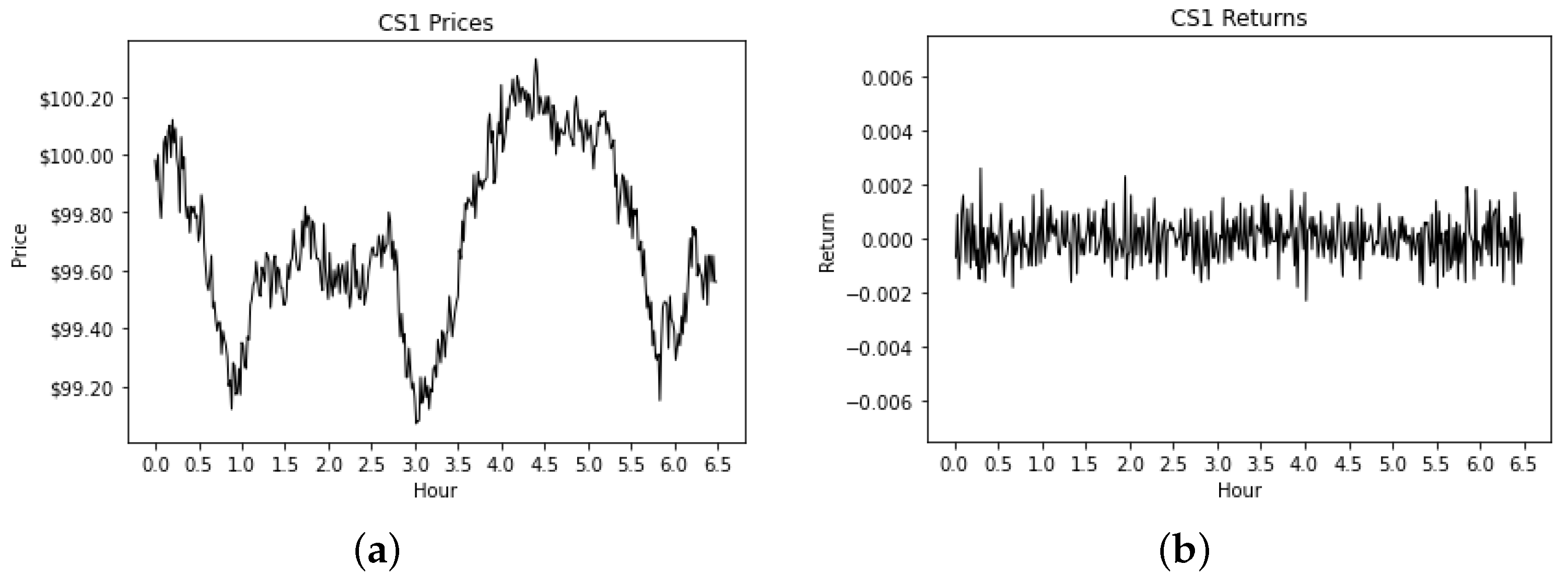
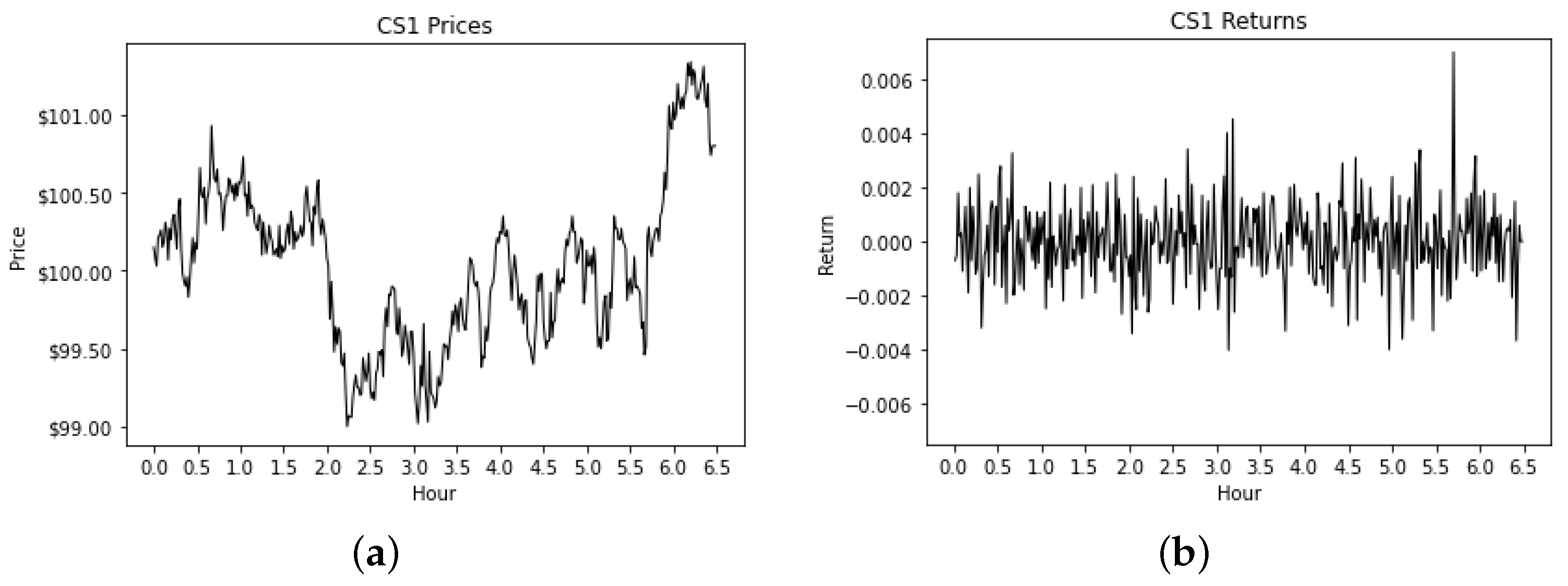
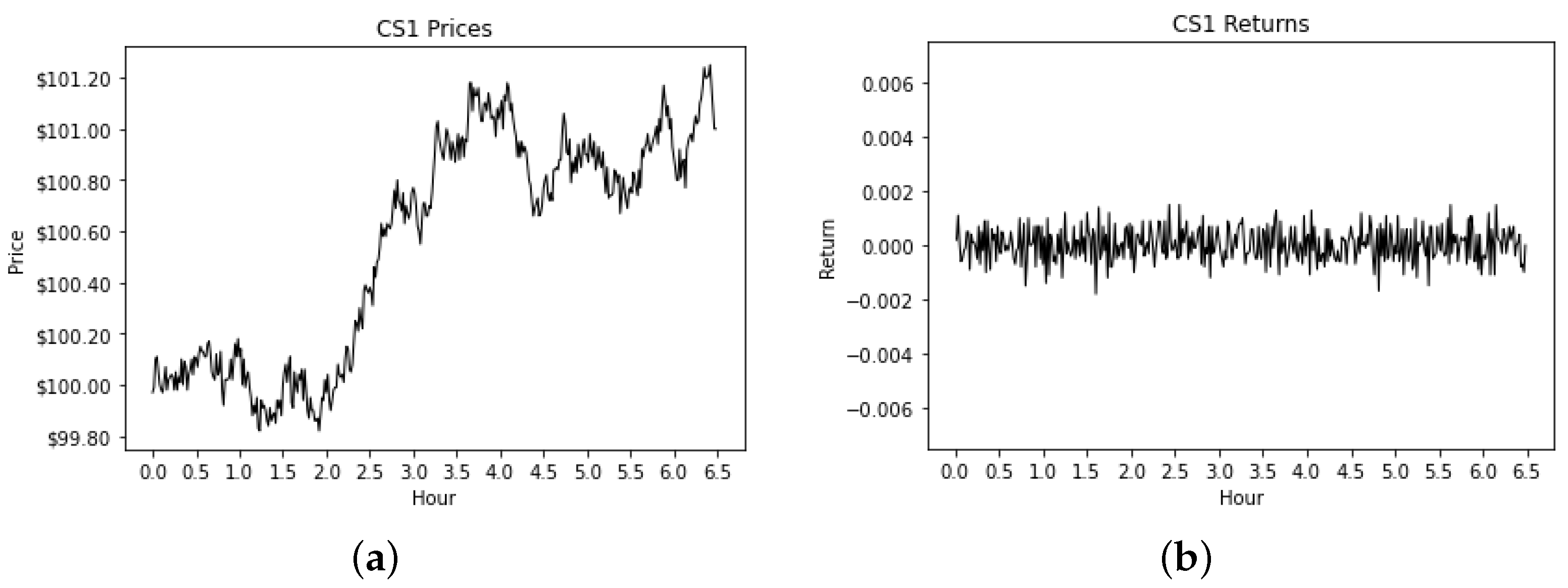
The examples of simulated price paths and returns are presented in
Figure 2,
Figure 3 and
Figure 4. The experiments in these figures share the same set of parameters, but, given the random nature of the simulations, the resulting price process is different every time the experiment is performed. These figures are depicting a homogeneous market with low activity—i.e., each trader submits limit orders once a minute on average.
Figure 2 is an experiment using continuous double auctions (CDA),
Figure 3 is an experiment using hidden volume continuous double auctions (HVCDA), and
Figure 4 is an experiment using frequent batch auctions (FBA) with 1-s batch intervals—hence, “FBA (
)” in the caption of
Figure 4.
We next perform a statistical analysis of the resulting time series, but we note that, visually, there is little difference among these figures. They all very much resemble real financial time series during a trading day. From the returns, it appears that FBA markets may have a lower volatility when compared to CDA markets, and that HVCDA markets may have a much higher volatility than either CDA and FBA markets, but these are based on a single experiment.
In the numerical results presented, we are considering several factors. As mentioned, we look at both homogeneous and heterogeneous markets. The second factor is market activity; we have low activity markets where traders submit limit orders on average every minute and high activity markets where orders are sent on average every half a minute. We also contrast different batch intervals, namely
,
,
, and
s. As previously mentioned in
Section 2.2, we understand the proposers of frequent batch auctions always aimed for sub-second batch intervals. As mentioned above, we hit a technical limitation regarding the amount of messages that need to be sent at the end of the batch auctions. This limits our capability to have auctions more frequently than 500 milliseconds.
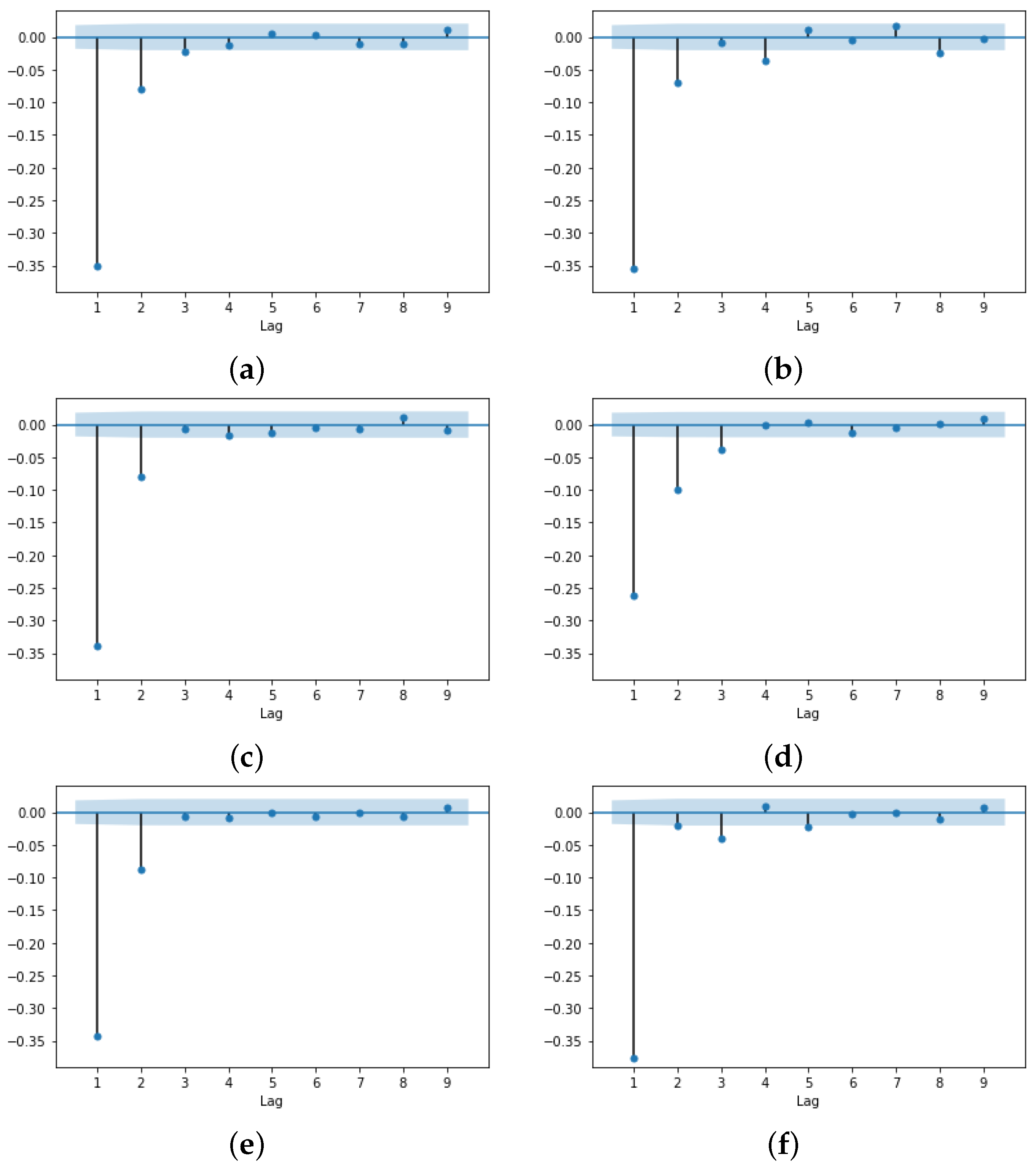
3.1.1. Resulting Return Dynamics
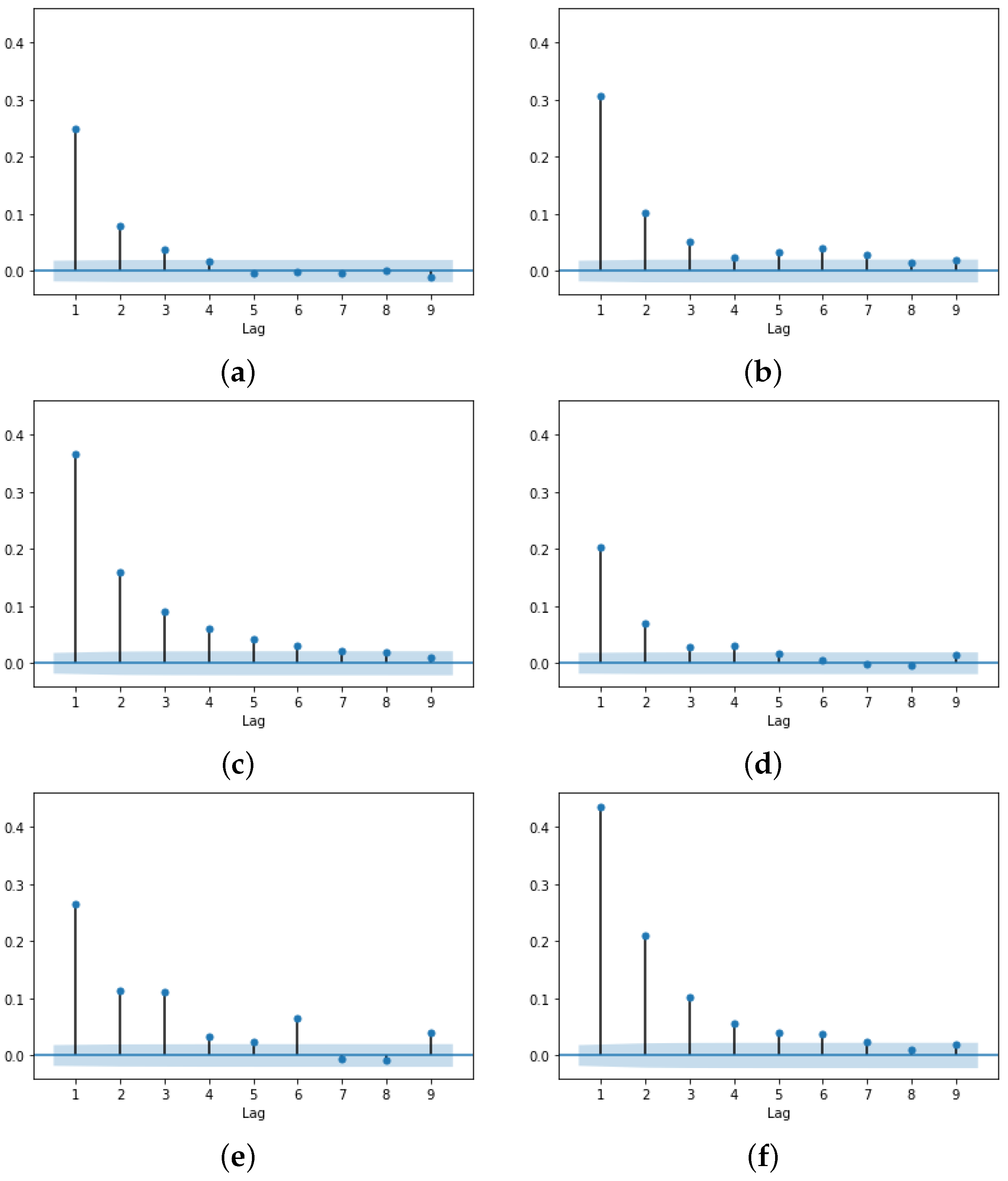
Figure 5,
Figure 6 and
Figure 7 showcase return statistics for the price evolution in
Figure 2b,
Figure 3b and
Figure 4b, as well as frequent batch auctions with batch intervals of
,
, and
s. We obviously cannot include all our simulations. The plots presented are representative of the results we typically obtain. In all plots, we use a sampling frequency of 2 s. This is to insure a proper comparison of the results, since the largest batch interval we are using is of 2 s. As highlighted in [
9], the sampling frequency plays a large role in the statistics of the results obtained.
In a typical market exchange (CDA), returns are negatively correlated due to the “bounce effect” caused by the bid–ask spread, since market orders are matching against both sides of the order book. Since the matching mechanism of FBA is completely different than CDA, we did not expect the results to be so close to the CDA. The HVCDA markets show a smaller first lag autocorrelation, which is understandable in a market where the only available information is the last price.
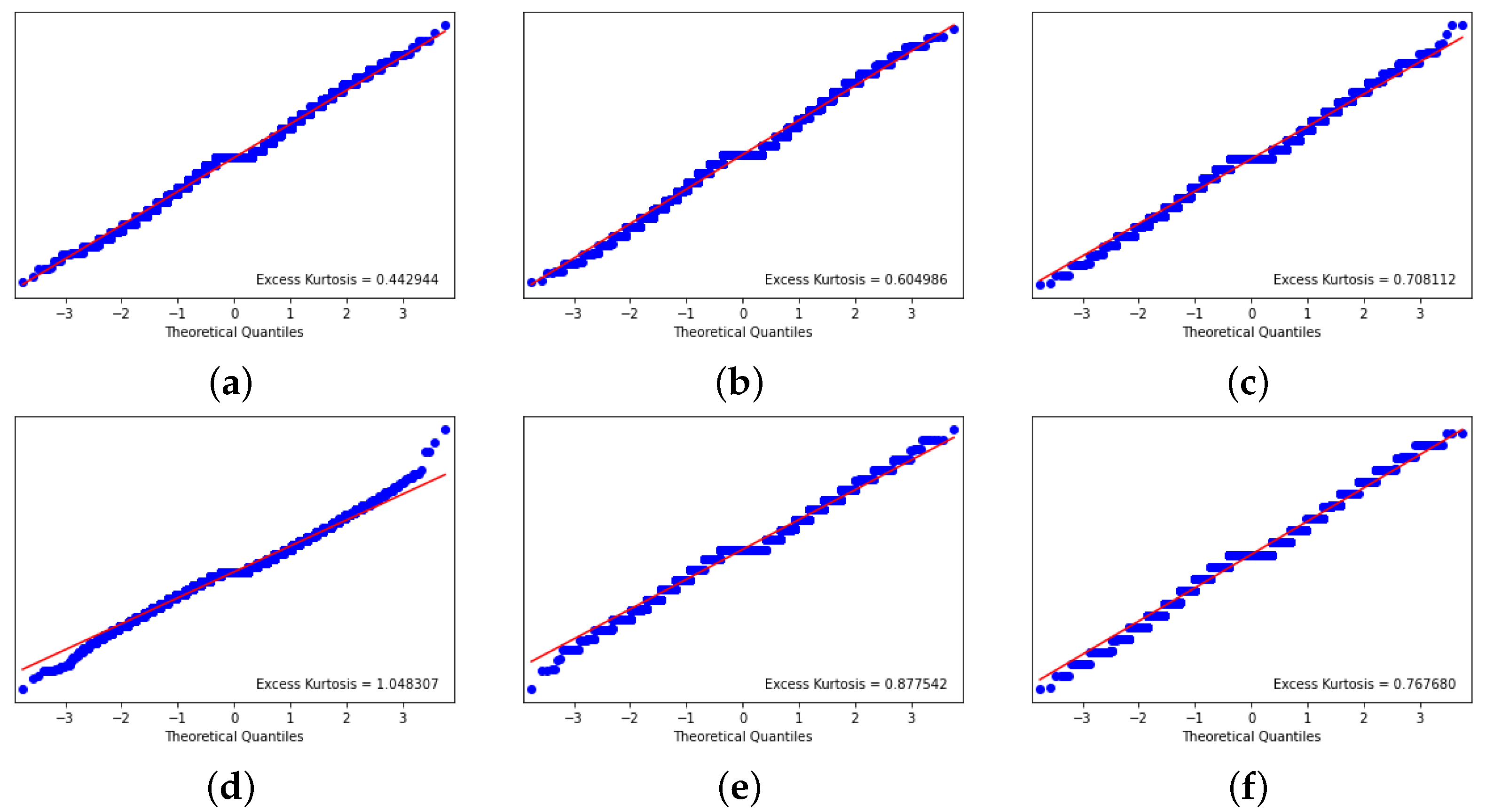
The returns in financial exchange markets are known to have a “heavy tails” (also known as leptokurtic) distribution [
25,
26]. In our results, all the returns from all the implemented markets have a leptokurtic distribution. The Q–Q plots in
Figure 6 and the numerical results in
Table 3 confirm it. In the table, the reported excess kurtosis values are averaged among all the experiments with the same combination of parameters. Even though not all the values are statistically different, we note an increasing trend in excess kurtosis as we move from CDA markets to FBA markets with a less frequent batch interval, regardless of the markets considered. We also note that excess kurtosis values for FBA seem to peak at FBA (
). The specific batch interval value (
s) is not too important, since it may be related to our experiment conditions, but the fact that we apparently reach a peak is interesting to investigate. The results obtained further indicate that excess kurtosis may be a parameter of interest when optimizing the batch interval in an FBA market. Finally, HVCDA markets present much higher excess kurtosis values when compared to any other market type.
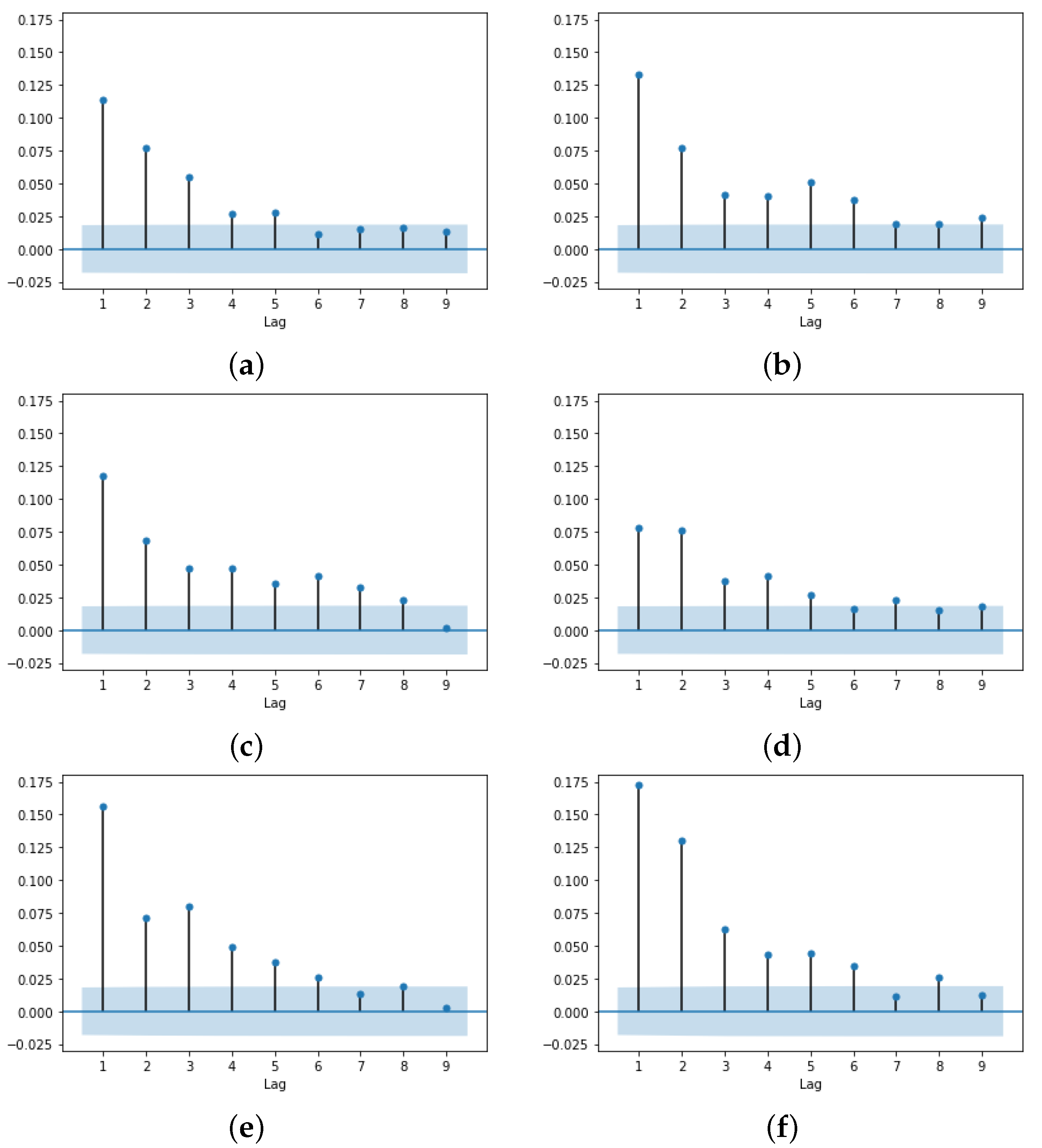
We are looking for the volatility clustering phenomenon documented in the literature [
27]. Again, the FBA plots are very similar to the CDA plot, including a slow decay in the autocorrelation of squared returns, which is a sign of long memory in the volatility [
28]. First, the lag autocorrelation is higher in the FBA markets than in the CDA markets, and the memory seems to last longer. All the time series generated by our experiments exhibit heteroskedastic effects, as determined by an ARCH test [
29], and the number of ARCH lags generally increases as we move from CDA markets to FBA markets with a less frequent batch interval. The average first lag squared returns autocorrelation and average number of ARCH lags required by each model are listed in
Table 3.
Table 3 also compiles the average realized volatility values for each experiment type we performed. As the return plots previously visually suggested (
Figure 4b vs.
Figure 2b), the FBA-realized volatility values tend to be lower when compared to CDA numbers, and these values decrease as we increase the batch interval length. Since the sampling frequency we used to compute the realized volatility is the same for every market type, the number of trades that happen during the day, which becomes lower as we increase the batch interval length, is not in effect here, but the frequency in which the information becomes available may be a factor. In HVCDA markets, where the only available information is the last traded price, and traders can only use this price as a basis for the prices of their orders, the realized volatility is significantly higher.
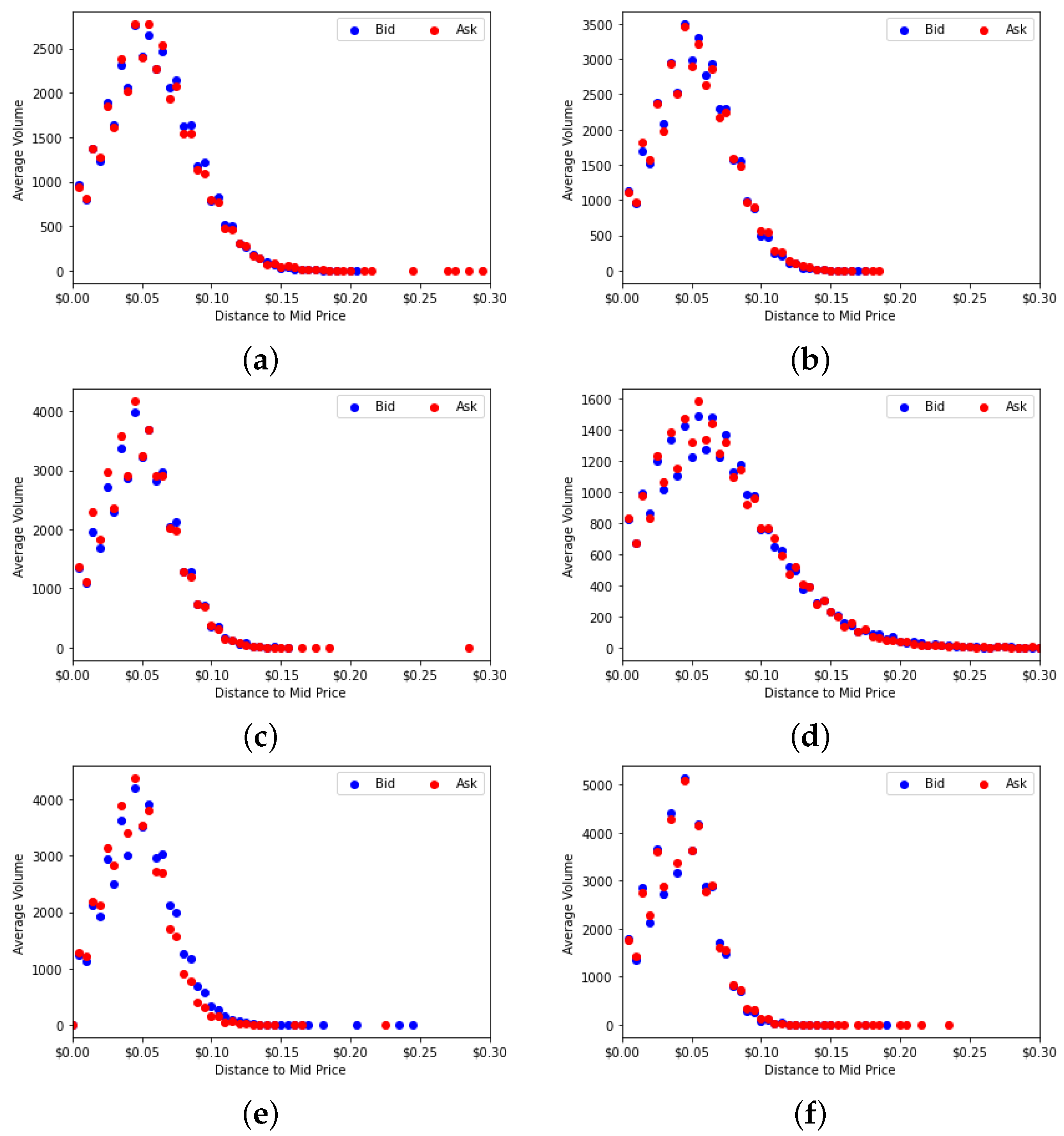
3.1.2. Limit Order Book Dynamics
After examining some of the typical stylized facts concerning the returns of time series, we next look at limit order book dynamics. Using the average volume at each tick away from the mid price, we plot the average shape of the limit order book [
30].
Figure 8 shows the examples of the average shape of the limit order book for each of the markets studied. The behaviors in both sides of the book are very similar. The peak a few ticks from the mid price is also anticipated, since orders at the top of the book will always be matched first, regardless of the market type.
Figure 8 shows the most glaring difference between market types that we observe so far. From the plots, we see that: as we change from CDA markets to FBA markets and as we decrease the batch interval frequency of these markets, the average shape of the order book becomes narrower. That is, the orders concentrate more around the mid price. Since traders do not receive constant updates of the new best prices, they concentrate their order prices around the last information they have. The more infrequent the market updates are, the more this holds true. In HVCDA, we see a completely opposite behavior: the limit order prices move away from the best prices. The mean and standard deviations of these distributions are reported in
Table 4. The same type of results are obtained regardless of the market setup (parameters).
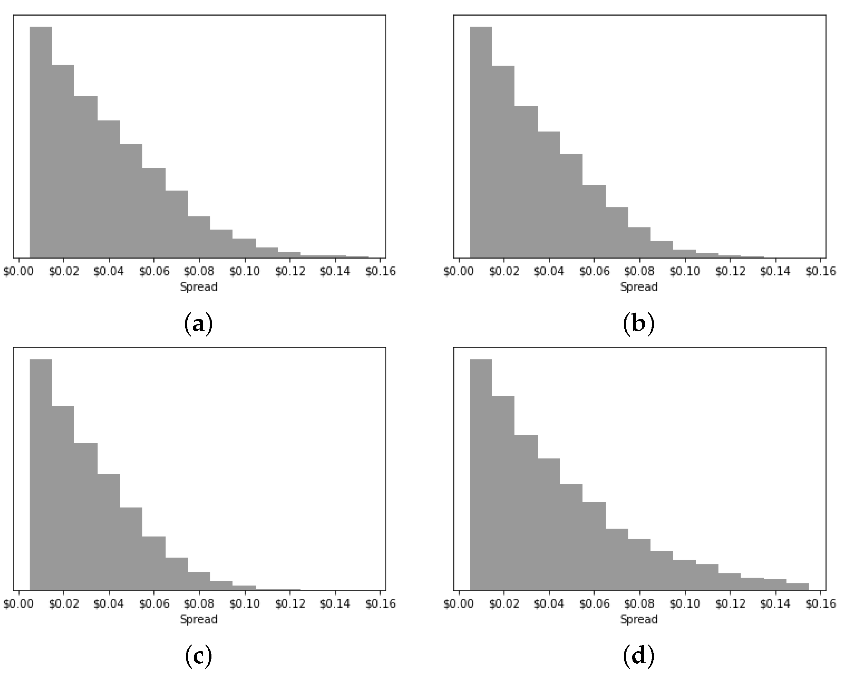
A very important measure is the spread (the difference between the best bid and best ask at any moment in time). The spread is commonly used as a criterion for both the liquidity and market quality [
12,
14]. Particularly, the spread autocorrelation (
Figure 9) should demonstrate signs of persistence [
31], and the spread distribution (
Figure 10) should show a power law asymptotic shape. The FBA markets display higher first lag autocorrelation values, and, similar to the volatility results, the memory of the spread time series is longer. The values for all market parameter combinations are presented in
Table 5.
The numerical statistics of the spread distribution in
Table 5 confirm the visual observations in
Figure 10. The FBA markets have a lower standard deviation of the spread when compared to CDA, while HVCDA has a much higher standard deviation. Apart from FBA (
), all other FBA markets present lower spread values (mean) and also consistently so (standard deviation). Using the spread as the measure of market quality, we can conclude that the FBA improve the market quality. In fact, we find that, in most cases, 1.5 s seems to be the best batch interval frequency for our setup. This is similar to our results obtained using kurtosis. We note that this value should be further investigated, as it probably depends on the available hardware. Nonetheless, the results point to the possibility of finding an optimal batch interval size using similar experiments.
Finally,
Table 5 also contains information on the average 95th percentile of the spread distribution for each market. We use this number as a proxy for the worst spread value. Similar to the results obtained above, FBA (
) seems to be a bad choice (at least in our configuration), but other FBA market configurations have better (lower) spread values. The HVCDA markets are the worse performers.
3.1.3. Orders Execution Information
All previous measures can be obtained from typical financial data. However, the SHIFT system contains account level information, and we can use this information to measure the market quality in a manner not possible using publicly available data. Different markets have different order execution profiles.
Table 6 summarizes the average number of traded shares for a given market, as well as the average execution time of liquidity providers and liquidity takers in these markets. Given the lack of market orders in FBA and the auctioning system, there is no way to distinguish between liquidity providers and liquidity takers in these markets.
Looking at the amount of shares traded, there is a significant difference between the CDA and HVCDA markets. This is even more evident in the more active markets. HVCDA markets have larger trading volume than any of the other markets we experiment with. Intuitively, the total amount of traded shares should drop for FBA markets, since there are less trading opportunities in these markets. However, in our experiments, the changes between different FBA markets appear to be negligible, and not that different from CDA. This is somewhat surprising.
HVCDA markets are also faster from the order execution time perspective, with averages much better than CDA markets. FBA order execution times seem to lie close to the average of the liquidity provider and liquidity taker average execution times in CDA markets. One might conclude that there is not much loss in the order execution time when moving from CDA to FBA markets. However, note that the promptness of market orders execution is obviously lost. As with the total amount of traded shares, it is interesting to note that, even though the execution time increases as we increase the batch interval length of FBA markets, the change is very small. This was unexpected, and it may indicate that the trading volume and the execution quality have less importance when looking for the optimal batch interval size.
3.2. Experiment 2: Market Stress Scenarios
In our second set of experiments, we study market reactions when receiving an exogenous shock mid operation. We performed a similar study in [
9], where we analyzed which of the four factors and their interactions were influential to market crashes. Here, we augment the experiment by adding another factor: the market type.
The setup is very similar to the one described in
Section 3.1. However, the total simulation time is
s (1 h). We do not need to simulate an entire trading day as we are limiting statistics to be impacted by the crash. New traders join the
traders about 30 min after the market opens. These new traders instigate a crash event at the 30 min mark, by placing large sell orders in the existing market. These new traders leave the market as soon as they liquidate their inventory. Next, we introduce the factors studied.
Market factors:
Market type: The market matching considered are continuous double auctions (CDA), frequent batch auctions (FBA), or hidden volume continue double auctions (HVCDA). For FBA, we only consider 1 s intervals (FBA ()), since this choice provides us with a good picture of the FBA results. Using multiple batch intervals would mean an increase in the total amount of experiments as well as add to the complexity of the analysis.
Trading frequency: Traders submit orders on average once a minute (1 min) or twice a minute (0.5 min).
Wealth homogeneity: The initial wealth of traders can be either homogeneously distributed (H), or non-homogeneously distributed (NH).
Crash condition factors:
Stress size: The total size of the orders placed by the stress traders in order to create the crash event is equivalent to either 5% (level one of the factor) or 10% (level two of the factor) of the total number of shares in the market.
Stress traders: This factor has three levels. The first level is a single stress trader submitting a large order (labeled 1 in our tables). The second level is constituted of a set of 20 such stress traders, all submitting their orders at the same time (20 s simultaneously). The third level consists of a similar set of 20 stress traders, but submitting their orders in 3-second intervals (20 NS non-simultaneously). The total size of the orders in the second and third level is equivalent to the size of the single order of the first level.
We performed a total of 720 experiments, 10 for each possible factor combination, which is 30 days worth of simulations. The results we gathered are stable and are presented in
Section 3.2.1 and
Section 3.2.2.
3.2.1. Market Drawdown Analysis
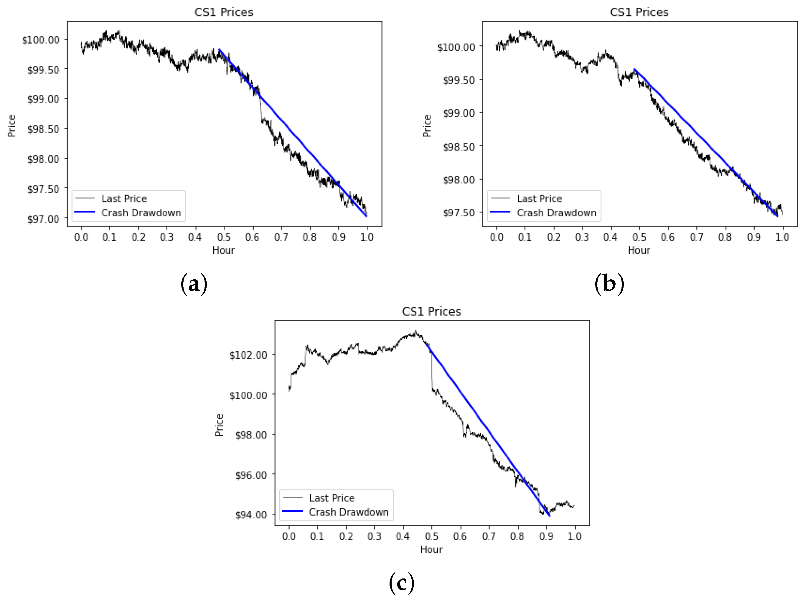
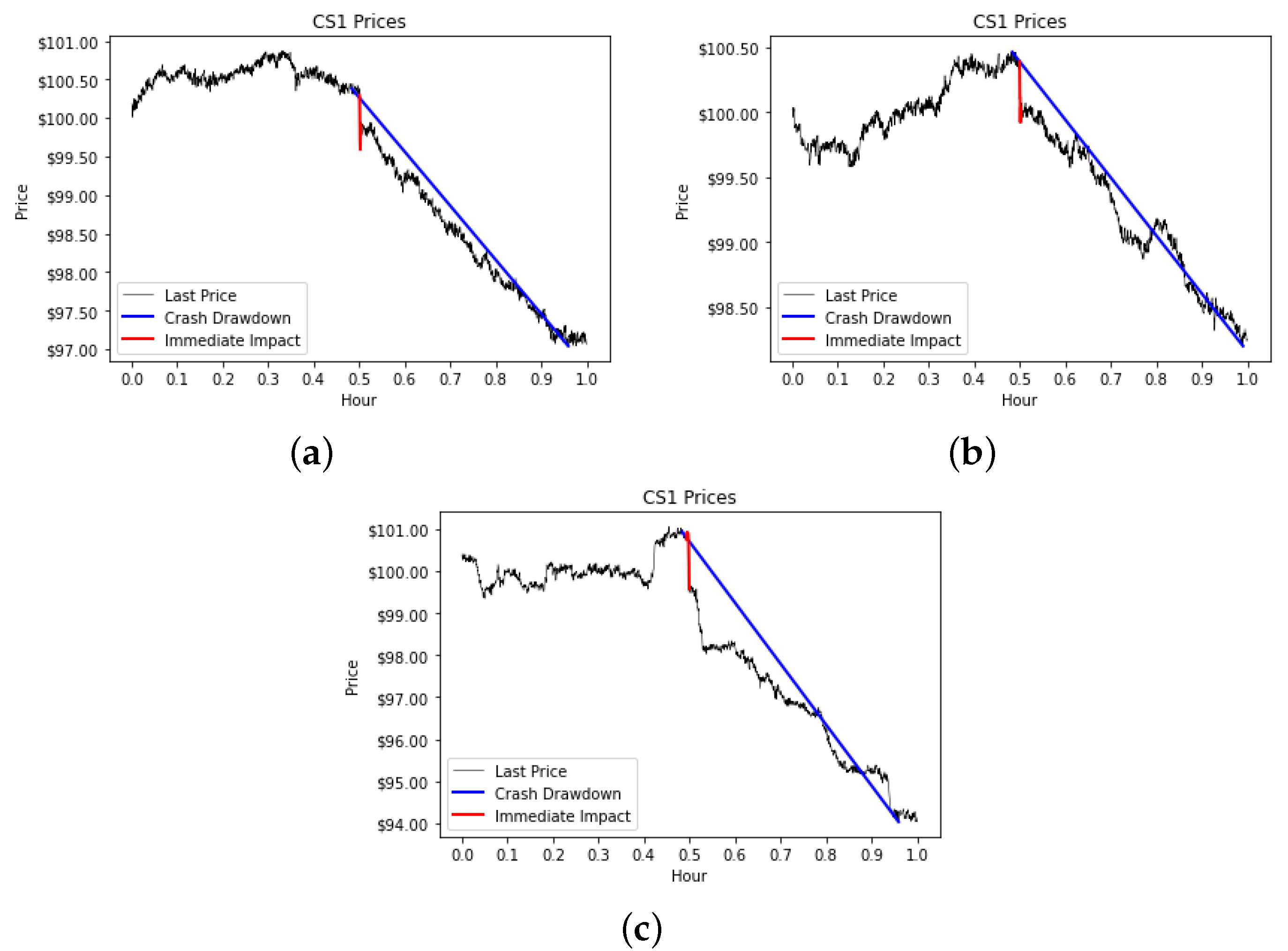
Some sample results of the simulated market crashes for each of the market types studied are shown in
Figure 11. The level values for all factors except the market type are kept the same. We see three different examples of pre-crash and post-crash market scenarios illustrated. In
Figure 11a, the market is stable before the crash. In
Figure 11b, the market price was already going down before the sell-off event, and the drop was exacerbated by the event. Finally, in
Figure 11c, the market price was increasing before the sell-off event, and there was a strong immediate impact at the moment of the crash. We discuss the concept of the immediate market impact in
Section 3.2.2.
In
Figure 11, all the market types are impacted by the sell event. This is a typical outcome in our experiments, particularly for those conducted with a large stress size (10%) and larger time interval (20 S stress traders), but it is not the only type of result we obtain.
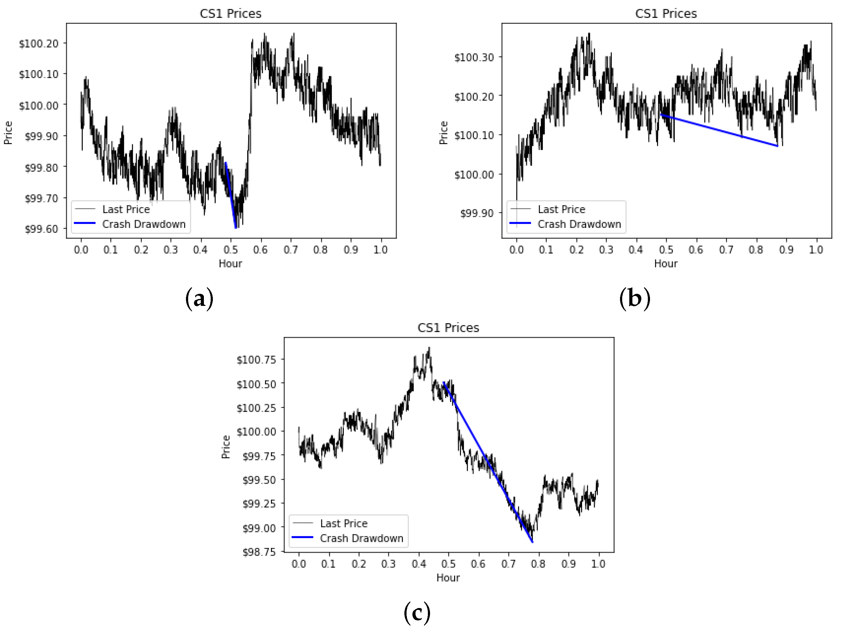
Figure 12 shows three results for experiments with other factor values (specified in the caption).
Figure 12a presents a market that is mostly unaffected by the orders from the stress traders, and that, in fact, has a very strong upward movement just after the event.
Figure 12b shows a market with no apparent change caused by the stress traders. In
Figure 12c, the market experiences a large loss, but the market recovers at the end. It is important to note that the plots we display in
Figure 11 and
Figure 12 are merely illustrative, and not indicative of performance in CDA, FBA, or HVCDA markets.
The point we are trying to illustrate in
Figure 11 and
Figure 12 is just how hard it is to analyze the resulting price path. We need to compute numerical values to help us identify and distinguish between the various resulting situations. In all the presented figures, we plot, in blue, the market drawdown slope caused by the crash event. We measure the drawdown caused by the crash starting one minute before the
known start time of the stress event. The slope is computed by dividing the drawdown magnitude by its duration.
In the first analysis presented in
Table 7, we use the drawdown slope as the response variable for our ANOVA. This slope is a proxy for both the magnitude as well as the duration of the market event; thus, we chose this numerical value to represent the impact of the crash.
Table 7 presents the final ANOVA model obtained after eliminating non-significant factors.
The results show that four out of the five factors are significant, as well as the interactions that are present among three of the factors. There is no evidence that wealth disparity among market participants impacts the size of the drawdown slope. Next we apply Tukey’s HSD test to the significant ANOVA factors.
Table 8 presents the results for the main factors, and
Table A1 (in the
Appendix A) for the interaction terms.
The most important result in
Table 8 is the comparison between market types. The market drawdown slope is significantly different for each market type. A lower slope value means that either the drawdown magnitude was small, or that it lasted longer and, thus, its impact was spread over a longer period of time. Looking at the results, the FBA markets have the least reaction to stress events. The HVCDA markets, on the other hand, seem to have the strongest expected market drawdown movement.
The results about the trading frequency and the stress size factors are as expected. More active markets (0.5 min) and larger stress events () will cause steeper drawdowns. Looking at the type of stress traders, the market stress caused by the 20 simultaneous traders (20 S) is in the middle and not significantly different than either the market stress generated by the single stress trader (1) or the 20 non-simultaneous stress traders (20 NS). However, the drawdown slope caused by the single trader is significantly larger than the one caused by the 20 non-simultaneous traders. As a parallel, consider consuming a dose of medicine all at once, divided it into 20 smaller ones all consumed consecutively, or spreading that dose into 20 to be consumed over certain time intervals. It would seem the first two approaches would have the same effect while the third is different.
However, in our previous study [
9], which did not include the FBA or HVCDA market types, we did not find any significant difference among either case with 20 stress traders, and both of them were significantly different than the case with a single trader. In that paper, we interpret the results as caused by the price–time order priority of the order-driven markets: “That is, the market order of the single stress trader will be executed in its entirety, all at once. The 20 orders from the 20 simultaneous traders are programmed to be submitted all at the same time. However, random orders from the other 200 market participants may arrive between these orders, thus sometimes smoothing the stress event effect. This in turn, produces statistically different results.”
The results we obtain now are caused by the introduction of new markets types in the experiments. In a batch auction type, if the 20 orders are sent simultaneously, they are likely to be processed within the same auction. As the orders are identical in price, they accumulate to a large order, likely to be similar to the one order received from the single trader. This is seen more clearly in
Table 9, where the statistics are conditioned on the market type. The results are not significant when conditioned—this may be an illustration of the Simpson’s paradox and the fact that interaction terms are significant. Nonetheless,
Table 9 shows how close the results for 20 simultaneous stress traders are to the results for 20 non-simultaneous stress traders in the CDA markets. It also shows that, in FBA markets, the results for a single stress trader are very close to the results for the 20 simultaneous stress traders. We believe these results add to our previous conclusions related to the price–time order priority effect of the order-driven markets.
We include the Tukey’s HSD test results for the interaction terms of the model in
Table A1, in the
Appendix A. When analyzing the trading frequency and stress size together, these terms interact. The larger stress events (
) in more active markets (0.5 min) produce a steeper drawdown movement than the individual level of factors separately.
The other conclusion we can draw from the interaction results is about the market type. If only CDA and FBA markets are considered, we obtain a similar conclusion, i.e., the combination of larger stress events in more active markets produce steeper market movements than individually. Further, the HVCDA markets are more susceptible to steeper drawdown movements than either CDA or FBA markets, regardless of the trading frequency of the market participants, or the stress size of the crash event.
3.2.2. Immediate Market Impact Analysis
The slope of the drawdown may be seen as a longer term impact. Here, we wanted to introduce a measure of immediate market impact.
Figure 12c on page 20 has an example of what we call an “immediate market impact”, i.e., a sharp price drop that is created by stress events.
Figure 13 presents several more examples, with the immediate market impact highlighted in red. Sometimes the market will recover a little after the large drop, even if it continues in a downward path afterward—
Figure 13a,b. Other times, the drop will be followed by another sharp drop, as in
Figure 13c. We are concerned with only the first,
immediate impact.
In our experiments, these immediate market impacts happen in about
of the cases. Clearly, manually looking for these is unfeasible with so many simulations; thus, we devised an automated procedure to detect them. The procedure was introduced in [
9] and it is presented in details therein. Here, we explain the intuition behind the procedure and we refer to the cited work for exact details. Since we know the time at which the large order(s) are placed, we look at the largest negative return in a window of time including this time. From the largest negative return, we look both backwards and forwards in time for larger than normal returns. The distribution of “Normal” returns is based on the return statistics of endogenous market scenarios with the same base parameters (wealth distribution, trading frequency, etc.). We are including both large negative and positive returns in this calculation, since either may be part of the stress event. The total final negative return must meet a threshold based on past statistics, otherwise the immediate market impact is set at 0.
We use this procedure to flag experiments with immediate market impacts. We create a binary response variable with value 1 if there was an immediate market impact and 0 if there was no immediate market impact. We then form a logistic model. From the analysis, we found that only the individual factors are important, with no significant interaction terms. Since interactions are not significant, the analysis may be simplified and
Table 10 presents the results of pairwise
t-tests performed for each of the individual factors.
Once again, the results show that HVCDA is not a good exchange type. These exchanges not only cause steeper drawdown movements when there is a market stress event, but, in of the cases, there will also be an immediate impact: double the rate of CDA and FBA markets. We also measure the average size of these immediate market impacts when they happen. The average size for HVCDA markets was , versus for CDA markets and only for FBA markets. Therefore, even though there is no significant difference in the probability of the immediate market impact for CDA compared to FBA, when they do happen, they are almost double in size than in the FBA markets. Again, the FBA markets stand out as a more stress-resistant alternative to CDA markets.
Different trading frequencies and wealth homogeneity profiles do not impact the probability of the immediate market impact. The results for the two remaining factors, stress size, and stress traders are again intuitive. The stress sizes of will cause immediate market impacts of the time, with an average drop size of , compared to stress sizes of causing immediate market impacts of the time, with an average impact size of . As for the stress traders, the results are similar to the drawdown slope results. There is no significant difference among a single trader and 20 simultaneous traders, with both causing immediate market impacts around of the time, against only when the stress event is caused by 20 non-simultaneous traders. The average impact sizes are around and , respectively.
4. Conclusions
This paper presents an attempt to implement the frequent batch auctions order-matching mechanism in a system that closely resembles a real market exchange in terms of functionality. The objective was to serve as a proof of concept for both FBA and SHIFT (our platform) as a means to experiment with policies before actual implementation. There are limitations to our study, as highlighted in
Section 2.2, and all the experiments were performed endogenously, with no source of outside information into the system. These laboratory conditions led us to interesting initial conclusions, not to be taken as proof of implementation at a real scale. Nonetheless, we believe studies similar to this are a necessary step in evaluating the feasibility of alternative market types such as frequent batch auctions (FBA). Furthermore, we were able to base our conclusions on market measures (trades and order books) as well as specific account level data (e.g., average execution time and provider and taker execution), which are not generally available for research.
Due to the sealed nature of the order submission stage of FBA markets, we created the HVCDA markets as sort of an FBA market limit, specifically when the limit of the batch interval time approaches zero. We thus included HVCDA in this study expecting to find some similarity in the obtained results. However, the actual results showed that the FBA markets are much closer statistically to the traditional CDA markets than we initially expected. Moreover, looking at common measures of market quality, the FBA markets seem to be a significant improvement in relation to CDA markets. The FBA markets are less uncertain, with lower volatility values, and more liquid, with tighter spread values. Of course, there is a loss of immediacy in order execution, but this would only be perceived by the actual target group of the FBA proposal: high-frequency traders. We also note that the results of our market stress experiments show how the FBA markets seem to be intrinsically better suited to resist crash events.
When working on these experiments, our objective was not to pinpoint the best batch interval length for frequent batch auctions, but we hoped we could obtain some insights. Our results indicate that going in the direction of more frequent auctions may not be the best solution. In fact, the results obtained indicate that it may be possible to optimize the batch interval based on a certain criteria. Such criteria should be based, among other things, on the market activity load of the target asset (volume and trading frequency). Different financial assets could probably benefit from using different batch interval sizes.
The FBA markets do, however, present some downsides, as they may prove to be technically challenging to implement in the real world. We mentioned the bottleneck we hit with FIX messages that did not allow us to try batch intervals of less than s. We understand this is probably a limitation of the hardware available to us, but similar issues (perhaps with a thinner time granularity) could arise in real market exchanges.
On this note, we also find it important to mention another issue we discovered while sampling data from FBA markets that could turn into a real issue for researchers and market participants. As we mentioned in
Section 2.2, the CDA order book updates can be sent to clients of the exchange as differentials from the previous information the clients already have. In FBA, the whole order book changes every time there is an auction and, thus, the entire book needs to be broadcasted. If a researcher or market participant is sampling the market using a constant frequency, it is possible that they sample the current bid order book and the previous ask order book, since the information may not have arrived or been processed by the client yet. This could be a serious issue, especially when sampling best prices or the spread (e.g., producing impossible negative spread values). Such inconsistencies are impossible with differential updates. A possible solution would be to have blackout periods when sampling is not possible or even allowed, which is yet another technical challenge.
We should mention that we started this study from the perspective of: “these academics that proposed FBA have no idea how markets are functioning in reality, let us dismantle this idea”. The results we obtained surprised us. We did not expect FBAs to perform so well, particularly when compared with an exchange model that has been functioning and continuously perfected for almost 100 years. The results completely transformed our perception of FBAs and, instead, caused us to become believers in this idea.
This study ended up by opening more doors than it closed. Future work includes exploring the few things we mentioned in the paper that would require further investigation, as well as a more thorough search for the optimal batch interval length of FBAs depending on the market parameters (traded stock volume and market participants).


