Min–Max Dynamic Programming Control for Systems with Uncertain Mathematical Models via Differential Neural Network Bellman’s Function Approximation

Abstract

This research focuses on designing a min–max robust control based on a neural dynamic programming approach using a class of continuous differential neural networks (DNNs). The proposed controller solves the robust optimization of a proposed cost function that depends on the trajectories of a system with an uncertain mathematical model satisfying a class of non-linear perturbed systems. The dynamic programming min–max formulation enables robust control concerning bounded modelling uncertainties and disturbances. The Hamilton–Jacobi–Bellman (HJB) equation’s value function, approximated by a DNN, permits to estimate the closed-loop formulation of the controller. The controller design is based on an estimated state trajectory with the worst possible uncertainties/perturbations that provide the degree of robustness using the proposed controller. The class of learning laws for the time-varying weights in the DNN is produced by studying the HJB partial differential equation. The controller uses the solution of the obtained learning laws and a time-varying Riccati equation. A recurrent algorithm based on the Kiefer–Wolfowitz method leads to adjusting the initial conditions for the weights to satisfy the final condition of the given cost function. The robust control suggested in this work is evaluated using a numerical example confirming the optimizing solution based on the DNN approximate for Bellman’s value function.

1. Introduction

The term optimal control refers to a group of techniques that can be used to create a control strategy that produces the best possible behaviour about the specified criterion (i.e., a strategy that minimizes a loss function). Two main techniques can define the solution of a given optimal control problem: maximal principle and dynamic programming. Pontryagin’s maximal principle gives a necessary condition for optimal outcomes [1]. Still, it cannot be used to derive close-loop solutions to the optimal control when the system is non-linear and is affected by modelling uncertainties and external perturbations [2].

On the other hand, the Hamilton–Jacobi–Bellman (HJB) provides a sufficient condition that can be used to arrive at the solutions of optimal control problems (see, for example, [3,4]. Both approaches, being theoretically elegant, have some significant drawbacks due to the requirement of precise knowledge of the system dynamics, which in practice includes internal uncertainties and external perturbations. When a mathematical model contains uncertain parameters from a priory given set, the formulation of necessary conditions for this case is known as the robust maximum principle [5]. The formulation of HJB equation under the presence of uncertainties/disturbances in the model description can be found in [6,7]. This robust version of the optimal control introduces novel approaches that can be exploited to consider no precise representations of the system that must be controlled. Moreover, it allows considering the effect of modelling uncertainties and external perturbations that satisfy some predefined bounds. Hence, using the robust HJB equations represents an innovation to solve online optimization problems that could usually be interpreted as an extremum-seeking control design problem. However, such solutions require a state-dependent explicit solution of the HJB equation, which is a complex task in general, considering that HJB is a non-linear partial equation [8,9].

In general, HJB equation cannot be solved analytically for non-linear mathematical models, even without the influence of errors or disturbances. Because of this, it was suggested in [10,11] that a numerical approximation of the relevant solution based on the use of static neural networks (NN) in which the NN weights are modified online by the least square method implementation [12,13]. From this point of view, this method is referred to as an adaptive realization of an optimal controller. This idea has been used in recent decades considering adaptive approximation of the value function associated with the HJB, which can offer an adaptive version of the optimization problem for dynamical systems. When the approximation is based on the introduction of artificial neural networks as an approximate model of the value function or the optimal structure, the technique is known as neural adaptive dynamic programming.

In this study, we suggest using a dynamic neural network (DNN) approach [14] for outline approximation of the Bellman’s function corresponding to the min–max solution of the HJB equation [15], where the maximum is taken over by the class of admissible uncertainty. The minimum is evaluated for the system trajectories affected by the worst internal parametric ignorance and the external bounded perturbations. Unlike static neural networks, which have weights that converge to "the optimal" approximate values, DNNs have changeable weights throughout the learning process. Utilizing the acquired necessary features [16], the entire design process may be achieved before applying the min–max control [17].

The main contributions of this study are:

-

Min–max formulation of the problem and the analytical calculation of the worst internal parametric uncertainties and external perturbations;

-

Development of the HJB equation corresponding to the considered min–max problem formulation;

-

Proposition of a DNN approximation for the solution of the HJB equation for the min–max problem;

-

Designing of the differential equations for the adjustment of the weights (learning) in the suggested DNN structure;

-

Numerical validation of the suggested method for some non-linear tested systems.

The structure of this manuscript is the following: Section 2 presents the problem formulation related to the type of non-linear system to be controlled and the min–max optimal control description. Section 3 presents the min–max formulation to design the proposed controller based on the approximate dynamic programming. Section 4 contains the estimation of the worst possible set of trajectories under the maximum value of external perturbations and modelling uncertainties. Section 5 establishes the robust version of the HJB equation evaluated over the estimated worst trajectories. Section 6 establishes the approximation of Bellman’s functions based on applying the DNN approximation capacities. Section 7 relates the DNN approximate values and its adjustment law, considering a recursive algorithm using the Kiefer–Wolfowitz method. Section 8 contains the final remarks and future trends based on the obtained results presented in this study.

2. Problem Formulation

Let us consider the non-linear controllable plant given by the following ordinary differential equation (ODE)

$$\dot{x}\left(t\right)=\left[A_0+\Delta A\left(x\left(t\right),t\right)\right]x\left(t\right)+B_{0}u+\eta \left(x\left(t\right),t\right),x_0=x\left(0\right),t\in [0,T],$$

(1)

where $x\in {\mathbb{R}}^n$ is the state vector, u$\in {\mathbb{R}}^m$ is the control action to be designed. The matrix $A_0\in {\mathbb{R}}^{n\times n}$ characterizes the internal linear relationship between the state and its dynamics. The matrix $B_0\in {\mathbb{R}}^{n\times m}$ defines the constant effect of control action u on the dynamics of the system. Time is represented by the variable t. The time window is defined by the finite value represented by T.

The internal uncertainty matrix $\Delta A\left(x\left(t\right),t\right):{\mathbb{R}}^n\times {\mathbb{R}}^{+}\to {\mathbb{R}}^{n\times n}$ is supposed to be bounded as follows

$$\underset{t\ge 0}{sup}{∥\Delta A\left(x\left(t\right),t\right)∥}^2\le {\alpha }^2.$$

(2)

here ${∥\Delta A\left(x\left(t\right),t\right)∥}^2:=\mathrm{tr}\left\{{\left(\Delta A\left(x\left(t\right),t\right)\right)}^{\top }\Delta A\left(x\left(t\right),t\right)\right\}$.

The non-measurable external disturbance is defined by $\eta \left(x\left(t\right),t\right):{\mathbb{R}}^n\times {\mathbb{R}}^{+}\to {\mathbb{R}}^n$. This term is also assumed to be bounded according to the following inequality:

$$\underset{t\ge 0}{sup}{∥\eta \left(x\left(t\right),t\right)∥}^2\le {\beta }^2.$$

(3)

Let the cost functional be given in the Bolza form:

$$J(0,x_0;u(·)):=h_0\left(x\left(T\right)\right)+\underset{t=0}{\overset{T}{\int }}h(x\left(t\right),u\left(t\right))dt,$$

(4)

with the quadratic cost functions

$$\left.\begin{array}{c}h(x,u)=x^{\top }Qx+u^{\top }Ru\\ \\ h_0\left(x\left(T\right)\right)=0.5x^{\top }\left(T\right)Sx\left(T\right)\end{array}\right\}.$$

(5)

Here the matrix $Q\in {\mathbb{R}}^{n\times n}$ is positive, semi-definite and symmetrical $(Q\ge 0,Q=Q^{\top })$, the control-associated matrix in the functional $R\in {\mathbb{R}}^{n\times n}$ is positive, definite and symmetrical $(R>0,R=R^{\top })$. The matrix related to the final condition $S\in {\mathbb{R}}^{n\times n}$ is positive, definite and symmetrical $(S>0,S=S^{\top })$.

This study designs the min–max control $u^{*}\in {\mathbb{R}}^m$ which must solve the following optimization problem

$$\underset{\left\{\Delta A,\eta \right\}\in {\mathrm{\Psi }}^{adm}}{max}J(0,x_0;u(·))\to \underset{u(·)\in U_{adm}[0,T]}{min},$$

subject to the dynamics given in Equation (1).

The set ${\mathrm{\Psi }}^{adm}$ defines the class of admissible internal uncertainties and external perturbations given by

$${\mathrm{\Psi }}^{adm}=\left\{\Delta A,\eta :\underset{t\ge 0}{sup}{∥\Delta A\left(x\left(t\right),t\right)∥}^2\le {\alpha }^2,\underset{t\ge 0}{sup}{∥\eta \left(x\left(t\right),t\right)∥}^2\le {\beta }^2\right\}.$$

(6)

The set $U_{adm}[0,T]$ consists of all piece-wise continuous vector functions $u\left(t\right)$ measurable (in the Lebesgue sense) for all $t\in [0,T]$. This means that the min–max optimal control is as follows:

$$u^{*}=\underset{u(·)\in U_{adm}[0,T]}{argmin}\underset{\left\{\Delta A,\eta \right\}\in {\mathrm{\Psi }}^{adm}}{max}J(0,x_0;u(·)).$$

(7)

3. HJB Min–Max Formulation

According to the results presented in [6,7], the sufficient condition for a control action u to be min–max (robust) optimal (7) consists of fulfilling the following max–min HJB equation [18,19]:

$$-{\displaystyle \frac{\partial V(t,x)}{\partial t}}+\underset{u(·)\in U_{adm}}{max}\underset{\left\{\Delta A,\eta \right\}\in {\mathrm{\Psi }}^{adm}}{min}H\left(-{\displaystyle \frac{\partial V(t,x)}{\partial x}},x,u,\Delta A,\eta \right)=0,$$

(8)

where the function $H:{\mathbb{R}}^n\times {\mathbb{R}}^n\times {\mathbb{R}}^m\times {\mathbb{R}}^{n\times n}\times {\mathbb{R}}^n\to \mathbb{R}$ is called the perturbed Hamiltonian (considering the effect of the parameters and external perturbations), which is given by

$$H(\psi ,x,u,\Delta A,\eta ):={\psi }^{\top }\dot{x}-h(x,u).$$

(9)

The vector $\psi$ is referred to as the adjoint variable satisfying the following differential equation with the corresponding final condition

$$\dot{\psi }=-\frac{\partial }{\partial x}H(\psi ,x,u,\Delta A,\eta ),\psi \left(T\right)={\left.\frac{d}{dx}{h}_0\left(x\right)\right|}_{x=x\left(T\right)}=Sx\left(T\right).$$

(10)

The value (Bellman) function V is defined for any $(0,x_0)\in [0,T)\times {\mathbb{R}}^n$ as

$$V(s,y):=\underset{u\in U_{adm}}{min}\underset{\left\{\Delta A,\eta \right\}\in {\mathrm{\Psi }}^{adm}}{max}J(s,y;u(·))$$

(11)

with the boundary condition

$$V(T,y)=h_0\left(y\right).$$

(12)

Here $h_0$ is defined in Equation (5).

4. Determination of the Worst Possible Uncertainty

Given the min–max formulation of the optimization problem considered in this study, it is necessary to estimate the state trajectories under the worst possible evolution of parametric uncertainties $\Delta A(x,t)$ and non-parametric imprecision, as well as external perturbations $\eta (x,t)$. This section presents this analysis.

Consider the following joint vector $\nu \left(x\left(t\right),t\right)$ defined as

$$\nu \left(x\left(t\right),t\right)=\left[\begin{array}{c}\Delta A\left(x\left(t\right),t\right)x\\ \eta \left(x\left(t\right),t\right)\end{array}\right].$$

The following lemma presents the result regarding the estimation of the mentioned worst possible trajectory:

Lemma 1.

The worst estimation

$${\nu }^{*}=\underset{\nu \in {\mathrm{\Psi }}^{adm}}{\mathrm{argmin}}\left\{{\psi }^{\top }\nu \left[\begin{array}{c}x\\ 1\end{array}\right]\right\},\psi =-{\displaystyle \frac{\partial }{\partial x}}V,$$

(13)

for the uncertainties/perturbation extended vector $\nu \left(x\left(t\right),t\right)$, as follows

$${\nu }^{*}\left(t\right)=\sqrt{{\alpha }^2+{\beta }^2}\frac{\psi \left(t\right)}{∥\psi \left(t\right)∥}\frac{{\left[\begin{array}{c}x\left(t\right)\\ 1\end{array}\right]}^{\top }}{∥\left[\begin{array}{c}x\left(t\right)\\ 1\end{array}\right]∥}.$$

(14)

Proof. 

In view of the Cauchy–Schwartz inequality [20] and Equations (2) and (3) we have the following upper estimate

$$\left|{\psi }^{\top }\nu \left[\begin{array}{c}x\\ 1\end{array}\right]\right|\le ∥\psi ∥∥\nu ∥∥\left[\begin{array}{c}x\\ 1\end{array}\right]∥\le \sqrt{{\alpha }^2+{\beta }^2}∥\psi ∥∥\left[\begin{array}{c}x\\ 1\end{array}\right]∥.$$

In view of the equality attainable for $\nu ={\nu }^{*}$ (14), the lemma is proven. □

Remark 1.

The "worst" trajectory $x^{*}$ (when $\nu ={\nu }^{*})$, the following auxiliary ordinary differential equation gives

$${\dot{x}}^{*}=A_0{x}^{*}+B_{0}u+{\nu }^{*}{\left[\begin{array}{cc}{\left[x^{*}\right]}^{\top }& 1\end{array}\right]}^{\top },x_0^{*}=x^{*}\left(0\right),t\in [0,T].$$

(15)

The initial condition $x^{*}\left(0\right)$ is a given constant vector. Notice that the dynamics (15) do not contain either uncertainty or perturbations. Therefore, these trajectories could be used to obtain the minimum value of the cost function using the standard dynamic programming approach based on HJB.

5. HJB Equation under the Effect of the Worst Possible Trajectories

Given Lemma 1, the following optimization problem arises for estimating the minimizing controller under the worst possible trajectory. The mathematical optimization technique known as dynamic programming has a necessary optimally derived condition from applying the Bellman equation. The payout from some initial decisions and the value of the decision problem that remains due to these initial choices is used to express the value (using the proposed Bellman function) of a decision problem at a specific time. Following Bellman’s principle of optimality, this divides a dynamic optimization issue into a series of better-defined sub-problems. Based on this technique, the optimization problem considered in this study can be solved based on the conjugated application of online optimization using the HJB with an approximated Bellman’s function [21,22].

According to the dynamic programming theory, and considering the application of the Hamiltonian function, the following equivalent problem for solving the optimal (under the worst possible uncertainties/perturbations) control $u^{*}$ can be proposed as follows:

$$\begin{array}{c}{u}^{*}\left(t\right)=\underset{u(·)\in U_{adm}[0,T]}{argmax}\underset{\nu \in {\mathrm{\Psi }}^{adm}}{argmin}H(\psi ,x,u,\nu )=\underset{u(·)\in U_{adm}[0,T]}{argmax}H({\psi }^{*},x^{*},u,{\nu }^{*})\\ {\psi }^{*}:=-{\left.{\displaystyle \frac{\partial V(t,x)}{\partial x}}\right|}_{x=x^{*}}.\end{array}$$

(16)

Given the arguments given in Equation (8), the robust optimal control $u^{*}$ is

$$u^{*}=-{\displaystyle \frac{1}{2}}{R}^{-1}{B}_0^{\top }{\left.{\displaystyle \frac{\partial V(t,x)}{\partial x}}\right|}_{x=x^{*}}.$$

(17)

Substituting both $u^{*}$ and ${\nu }^{*}$ in the HJB equation leads to:

$$\begin{array}{c}-{\displaystyle \frac{\partial V(t,x^{*})}{\partial t}}-{\left({\displaystyle \frac{\partial V(t,x^{*})}{\partial x}}\right)}^{\top }{A}_0{x}^{*}+{\displaystyle \frac{1}{4}}{\left({\displaystyle \frac{\partial V(t,x^{*})}{\partial x}}\right)}^{\top }{B}_0{R}^{-1}{B}_0^{\top }{\displaystyle \frac{\partial V(t,x^{*})}{\partial x}}\\ -\parallel x^{*}{\parallel }_Q^2-\sqrt{{\alpha }^2+{\beta }^2}{\left({\displaystyle \frac{\partial V(t,x^{*})}{\partial x}}\right)}^{\top }{\displaystyle \frac{{\displaystyle \frac{\partial V(t,x^{*})}{\partial x}}}{∥{\displaystyle \frac{\partial V(t,x^{*})}{\partial x}}∥}}{\displaystyle \frac{{\left[\begin{array}{c}{x}^{*}\\ 1\end{array}\right]}^{\top }}{∥\left[\begin{array}{c}{x}^{*}\\ 1\end{array}\right]∥}}\left[\begin{array}{c}{x}^{*}\\ 1\end{array}\right]=0.\end{array}$$

Using a simplification process on the last term of the right-hand side of the previous partial differential equation leads to

$$\begin{array}{c}-{\displaystyle \frac{\partial V(t,x^{*})}{\partial t}}-{\left({\displaystyle \frac{\partial V(t,x^{*})}{\partial x}}\right)}^{\top }{A}_0{x}^{*}+{\displaystyle \frac{1}{4}}{\left({\displaystyle \frac{\partial V(t,x^{*})}{\partial x}}\right)}^{\top }{B}_0{R}^{-1}{B}_0^{\top }{\displaystyle \frac{\partial V(t,x^{*})}{\partial x}}\\ -\parallel x^{*}{\parallel }_Q^2-\sqrt{{\alpha }^2+{\beta }^2}∥{\displaystyle \frac{\partial V(t,x^{*})}{\partial x}}∥\sqrt{{∥x^{*}∥}^2+1}=0.\end{array}$$

(18)

The solution for the Bellman’s function $V(t,x^{*})$ in Equation (18) is tough to find analytically. That is why we propose to use DNN approximation for $V(t,x^{*})$, which is explained in the next section.

6. Bellman’s Function DNN Approximation

Consider the representation $V(t,x^{*})\simeq V_a(t,x^{*})$ for the Bellman’s function. The function $V_a(t,x)$ is an approximate solution associated with the HJB Equation (18) that satisfies the following DNN structure:

$$V_a(x^{*},t)={\omega }^{\top }\left(t\right)\sigma \left(x^{*}\right)+{\left[x^{*}\right]}^{\top }P\left(t\right)x^{*}.$$

(19)

In Equation (19), the matrix $P\in {\mathbb{R}}^{n\times n}$ is a positive definite solution, which is uniformly bounded with respect to time $t\in {\mathbb{R}}^n$ and $\sigma \in {\mathbb{R}}^n$ are associated with the DNN weights and activation functions, respectively. The components of $\sigma$ are selected strictly for positive sigmoidal functions.

The substitution of the approximate Bellman’s function $V_a(x^{*},t)$ in Equation (18) leads to

$$\begin{array}{c}-{\left[x^{*}\right]}^{\top }\dot{P}\left(t\right)x^{*}-{\dot{\omega }}^{\top }\left(t\right)\sigma \left(x^{*}\right)-{\omega }^{\top }\left(t\right){\displaystyle \frac{d}{dx}}{\sigma }^{\top }\left(x^{*}\right)A_0{x}^{*}-2{\left[x^{*}\right]}^{\top }P\left(t\right)A_0{x}^{*}\\ +{\displaystyle \frac{1}{4}}\left({\omega }^{\top }\left(t\right){\displaystyle \frac{d}{dx}}\sigma \left(x^{*}\right)+2{\left[x^{*}\right]}^{\top }P\left(t\right)\right)B_0{R}^{-1}{B}_0^{\top }\left({\displaystyle \frac{d}{dx}}{\sigma }^{\top }\left(x^{*}\right)\omega \left(t\right)+2P\left(t\right)x^{*}\right)\\ -\sqrt{{\alpha }^2+{\beta }^2}\sqrt{\left(\parallel x^{*}{\parallel }^2+1\right)}∥{\displaystyle \frac{d}{dx}}{\sigma }^{\top }\left(x^{*}\right)\omega \left(t\right)+2P\left(t\right)x^{*}∥-{\parallel x^{*}\parallel }_Q^2\simeq 0.\end{array}$$

(20)

Introducing the unitary and finite valued term ${\displaystyle \frac{{\sigma }^{\top }\left(x^{*}\left(t\right)\right)}{{∥\sigma \left(x^{*}\left(t\right)\right)∥}^2}}\sigma \left(x^{*}\left(t\right)\right)$ in the components that contain $\omega \left(t\right)$ in Equation (20) yields

$$\begin{array}{c}-{\dot{\omega }}^{\top }\left(t\right)\sigma \left(x^{*}\left(t\right)\right)-{\omega }^{\top }\left(t\right){\displaystyle \frac{d}{dx}}\sigma \left(x^{*}\left(t\right)\right)A_0{x}^{*}\left(t\right){\displaystyle \frac{{\sigma }^{\top }\left(x^{*}\left(t\right)\right)}{{∥\sigma \left(x^{*}\left(t\right)\right)∥}^2}}\sigma \left(x^{*}\left(t\right)\right)+\\ {\displaystyle \frac{1}{4}}{\omega }^{\top }\left(t\right){\displaystyle \frac{\partial }{\partial x}}\sigma \left(x^{*}\left(t\right)\right)B_0{R}^{-1}{B}_0^{\top }{\left({\displaystyle \frac{d}{dx}}\sigma \left(x^{*}\left(t\right)\right)\right)}^{\top }\omega \left(t\right){\displaystyle \frac{{\sigma }^{\top }\left(x^{*}\left(t\right)\right)}{{∥\sigma \left(x^{*}\left(t\right)\right)∥}^2}}\sigma \left(x^{*}\left(t\right)\right)+\\ {\left[x^{*}\left(t\right)\right]}^{\top }P\left(t\right)B_0{R}^{-1}{B}_0^{\top }{\left({\displaystyle \frac{d}{dx}}\sigma \left(x^{*}\left(t\right)\right)\right)}^{\top }\omega \left(t\right){\displaystyle \frac{{\sigma }^{\top }\left(x^{*}\left(t\right)\right)}{{∥\sigma \left(x^{*}\left(t\right)\right)∥}^2}}\sigma \left(x^{*}\left(t\right)\right)+\\ -\sqrt{{\alpha }^2+{\beta }^2}\sqrt{\left(\parallel x^{*}{\left(t\right)\parallel }^2+1\right)}∥{\displaystyle \frac{d}{dx}}{\sigma }^{\top }\left(x^{*}\right)\omega \left(t\right)+2P\left(t\right)x^{*}\left(t\right)∥{\displaystyle \frac{{\sigma }^{\top }\left(x^{*}\left(t\right)\right)}{{∥\sigma \left(x^{*}\left(t\right)\right)∥}^2}}\sigma \left(x^{*}\left(t\right)\right)\simeq 0.\end{array}$$

(21)

Based on the introduction of the unitary term presented above, the strategy simplifies and removes some of the practical implementations of previous robust optimal control designs using neural network approximations [7,23]. Notice that the expression presented in Equation (21) contains several terms that are proportional to the $\sigma \left(x^{*}\left(t\right)\right)$. Reorganizing the last expression as ${\left(·\right)}^{\top }\sigma \left(x^{*}\left(t\right)\right)=0$, we may conclude that $\left(·\right)=0$. This strategy is commonly implemented in the design of learning laws for a DNN as mentioned in [14,24]. Hence, based on this strategy, it is feasible to estimate the temporal evolution of the weights according to the following ordinary differential equation, which defines the dynamics of all components in $\omega \left(t\right)$:

$$\begin{array}{c}\dot{\omega }\left(t\right)={\displaystyle \frac{\sigma \left(x^{*}\left(t\right)\right)}{{∥\sigma \left(x^{*}\left(t\right)\right)∥}^2}}\mathrm{\Omega }\left(x^{*}\left(t\right),\omega \left(t\right)\right)\\ \\ \mathrm{\Omega }\left(x^{*}\left(t\right),\omega \left(t\right)\right)=-\left[{\left(x^{*}\left(t\right)\right)}^{\top }{A}_0^{\top }{\left({\displaystyle \frac{d}{dx}}\sigma \left(x^{*}\left(t\right)\right)\right)}^{\top }\omega \left(t\right)\right]+\\ {\displaystyle \frac{1}{4}}\left[{\omega }^{\top }\left(t\right)\left({\displaystyle \frac{d}{dx}}\sigma \left(x^{*}\left(t\right)\right)\right)B_0{R}^{-1}{B}_0^{\top }{\left({\displaystyle \frac{\partial }{\partial x}}\sigma \left(x^{*}\left(t\right)\right)\right)}^{\top }\omega \left(t\right)\right]+\\ \left[{\omega }^{\top }\left(t\right){\displaystyle \frac{d}{dx}}\sigma \left(x^{*}\left(t\right)\right)B_0{R}^{-1}{B}_0^{\top }P\left(t\right)x^{*}\left(t\right)\right]-\\ \sqrt{{\alpha }^2+{\beta }^2}\sqrt{\left(\parallel x^{*}{\left(t\right)\parallel }^2+1\right)}∥{\left({\displaystyle \frac{d}{dx}}\sigma \left(x^{*}\left(t\right)\right)\right)}^{\top }\omega \left(t\right)+2P\left(t\right)x^{*}\left(t\right)∥\\ \\ \omega \left(T\right)=0,\omega \left(t\right)\in {\mathbb{R}}^n.\end{array}$$

(22)

Hence, based on the definition of $\mathrm{\Omega }\left(x^{*}\left(t\right),\omega \left(t\right)\right)$ (which is known as the learning law), Equation (20) admits the following representation for the HJB equation using the approximate representation of the Bellman’s function:

$${\left[x^{*}\right]}^{\top }\mathrm{Ric}\left(P\right)x^{*}+\left(\dot{\omega }\left(t\right)-{\displaystyle \frac{\sigma \left(x^{*}\left(t\right)\right)}{{∥\sigma \left(x^{*}\left(t\right)\right)∥}^2}}\mathrm{\Omega }\left(x^{*}\left(t\right),\omega \left(t\right)\right)\right)\sigma \left(x^{*}\left(t\right)\right)\simeq 0,$$

(23)

where the expression $\mathrm{Ric}\left(P\right)$ described the following matrix Riccati differential equations given by

$$\mathrm{Ric}\left(P\right)=-\dot{P}\left(t\right)-P\left(t\right)A_0-A_0^{\top }P\left(t\right)+P\left(t\right)B_0{R}^{-1}{B}_0^{\top }P\left(t\right)-Q=0$$

(24)

Taking into account the Property (12), the initial conditions for $\omega \left(0\right)$ and $P\left(0\right)$ should be selected in such a way the following final conditions could be met

$$\omega \left(T\right)=0\mathrm{and}P\left(T\right)=S.$$

(25)

So, based on the presented results, we are now ready to formulate the principal result of this study.

Theorem 1.

If adjustment laws for the parameters in the DNN are given by Equation (22) and the time-dependent Riccati Equation (24) has a positive definite solution P with the initial conditions and $P\left(0\right)$, providing the Property (25), then $V_a(x^{*},t)$ gives the approximation of the Bellman’s function $V(x^{*},t).$

Since both ODE (22) and (24) have the terminal Conditions (25) we need to apply a recursive method (in this case, the “shooting” method) to find the appropriate initial conditions $\omega \left(0\right)$ and $P\left(0\right)$. Notice that the ODE $\mathrm{Ric}\left(P\right)=0$ (24) can be resolved in inverse time $\tau =T-t$ using the initial condition for $\tau =0$ which is $P\left(T\right)=S$. So, fulfilling of the terminal condition for Equation (24) does not present any problem. In the next section, we will discuss the recursive method for finding initial the condition $\omega \left(0\right)$ realizing the terminal requirements $\omega \left(T\right)=0$. In view of the approximated model Equation (19), finally, the robust control $u^{*}$ may be represented as

$$u^{*}\left(t\right)=-{\displaystyle \frac{1}{2}}{R}^{-1}{B}_0^{\top }\left(\frac{d}{dx}{\sigma }^{\top }\left(x^{*}\left(t\right)\right)\omega \left(t\right)+2P\left(t\right)x^{*}\left(t\right)\right),$$

(26)

where $x^{*}\left(t\right)$ and $\omega \left(t\right)$ are given by Equations (15) and (22), respectively, including $P\left(t\right)$ as in Equation (24).

7. Recursive Method to Realize the Terminal Conditions for the Weight Dynamics

The exact dependence of the performance index $J(0,x_0^{*};u^{*}(·))$ (4) on $\omega \left(0\right)$ is difficult to be obtained analytically. This condition constrains the application of traditional recurrent optimization algorithms such as gradient descendent [25] or Levenberg–Marquardt methodology [26]. As an alternative, here we apply the so-called, modified deterministic Kiefer–Wolfowitz method [27,28] applied to the optimization performance index considering that $J(0,x_0^{*};u^{*}(·)$= J$\left(\omega \right(0\left)\right)$. The following describes this method’s recursive procedure:

$$\left.\begin{array}{c}{\omega }_k\left(0\right)={\omega }_{k-1}\left(0\right)-{\displaystyle \frac{{\gamma }_k}{{\alpha }_k}}\left(Y_k({\omega }_{k-1}\left(0\right),{\alpha }_k)-Y_k({\omega }_{k-1}\left(0\right),0\right)\\ \\ Y_k({\omega }_{k-1}\left(0\right),{\alpha }_k)={\left(Y_{k,1}({\omega }_{k-1}\left(0\right),{\alpha }_k),\cdots ,Y_{k,n}({\omega }_{k-1}\left(0\right),{\alpha }_k)\right)}^{\top }\\ Y_{k,i}({\omega }_{k-1}\left(0\right),{\alpha }_k)=J({\omega }_{k-1}\left(0\right)+{\alpha }_k{e}_i),e_i=\left(\underset{i}{\underbrace{0,\dots ,0,1}},0,\dots ,0\right)\\ {\displaystyle \sum _{k=1}^{\infty }{\gamma }_k=\infty ,\sum _{k=1}^{\infty }{\alpha }_k=\infty ,\sum _{k=1}^{\infty }{\gamma }_k{\alpha }_k<\infty ,{\gamma }_k,{\alpha }_k>0.}\end{array}\right\}$$

(27)

In this function, ${\gamma }_k$ can be selected as a small constant and ${\alpha }_k={\alpha }_0{k}^{-\alpha },$$0<\alpha \le 1$. From a practical point of view, both parameters ${\gamma }_k$ and ${\alpha }_k$ can be selected as small constants.

The evolution of this algorithm allows the adjustment of the initial weights of the DNN running at each step of the recurrent methodology. The combination of this recurrent strategy running in discrete form and the continuous evolution of the system controlled with the approximate value of the Bellman’s function based on the DNN appear to be a class of hybrid system. Moreover, adjusting the initial weights in each recurrent stage, driving the performance function towards its minimum value, seems to operate as a class of reinforcement learning using the Kiefer–Wolfowitz method.

A simple diagram of the hybrid algorithm is shown in Figure 1. This diagram shows the two outer loops that define how the recurrent method works over the continuous development of the proposed min–max optimized controller.

8. Numerical Example

The following parameters of the model presented in Equation (1) were considered for numerical evaluation purposes:

$$\begin{array}{c}{A}_0=\left[\begin{array}{cc}-1.0& 0.5\\ 0.0& 2.0\end{array}\right],B_0=\left[\begin{array}{c}1\\ 1\end{array}\right]\\ \Delta A\left(x\left(t\right),t\right)={\epsilon }_1\left[\begin{array}{cc}{\displaystyle \frac{x_1^2}{x_1^2+1}}& ta{n}^{-1}\left(x_2\right)\\ 0.5sin\left({\omega }_{A}t\right)& 0\end{array}\right]\\ \eta \left(x\left(t\right),t\right)={\epsilon }_2\left[\begin{array}{c}sin\left({\omega }_{1}t+{\varphi }_1\right)\\ sin\left({\omega }_{2}t+{\varphi }_2\right)\hfill \end{array}\right].\end{array}$$

The model with uncertain mathematical structure was simulated in Matlab/Simulink using the ODE-01 (Euler) integration method with the integration step fixed to 0.001 s.

The proposed modified deterministic Kiefer–Wolfowitz method was implemented in M-language in Matlab to perform the recurrent scheme described in Equation (27). The number of cycles evaluated for this recurrent algorithm was $k=3900.$

The evolution of the states $x_1$ and $x_2$ appears in Figure 2 and Figure 3. These figures compare the evolution of the worst trajectories $x_1^{*}$ and $x_2^{*}$ considering the upper bound of the admissible perturbations. Notice that both states are moving towards the origin. Still, in the case of the worst trajectories, there are no oscillations in the steady state in opposition to the controlled states that are affected by the selected uncertainties and perturbations. Furthermore, one may notice that the first variable has a more evident difference between the worst estimated trajectories for the controlled ones. The trajectories for $x_1$ and $x_2$ correspond to those generated with the final weights derived at the end of the iteration process endorsed with the Kiefer–Wolfowitz strategy.

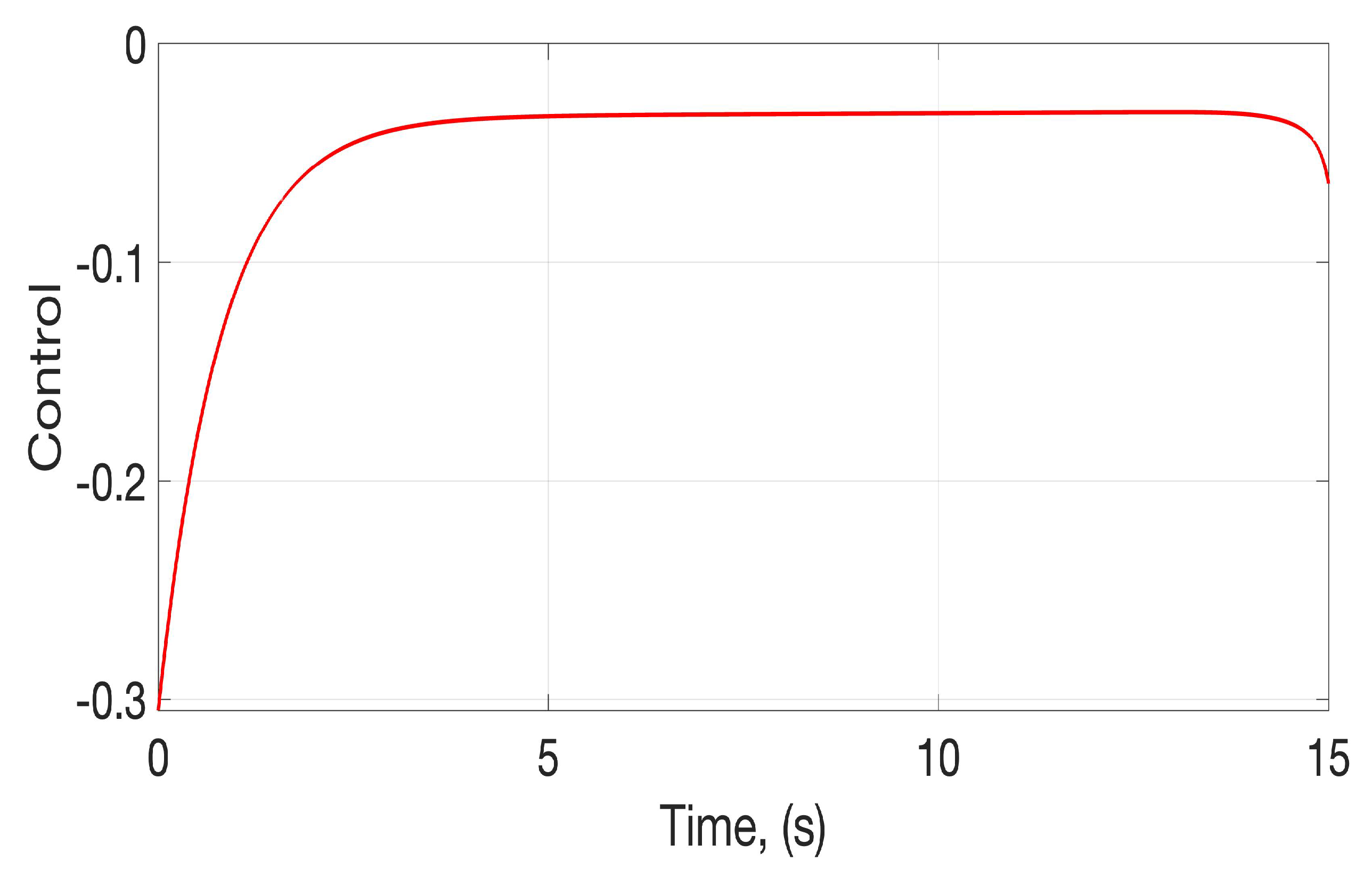
The evolution of the states shown in Figure 2 and Figure 3 are generated by the control action depicted in Figure 4, that is the result produced when the complete set of iterations in the Kiefer–Wolfowitz algorithm is ended. This controller also responds to the effect of uncertainties and perturbations, limiting the possibility that the control action converges towards the origin. Nevertheless, the obtained control action corresponds to the outcome endorsed after the iterative algorithm ends, reaching the early stop criterion.

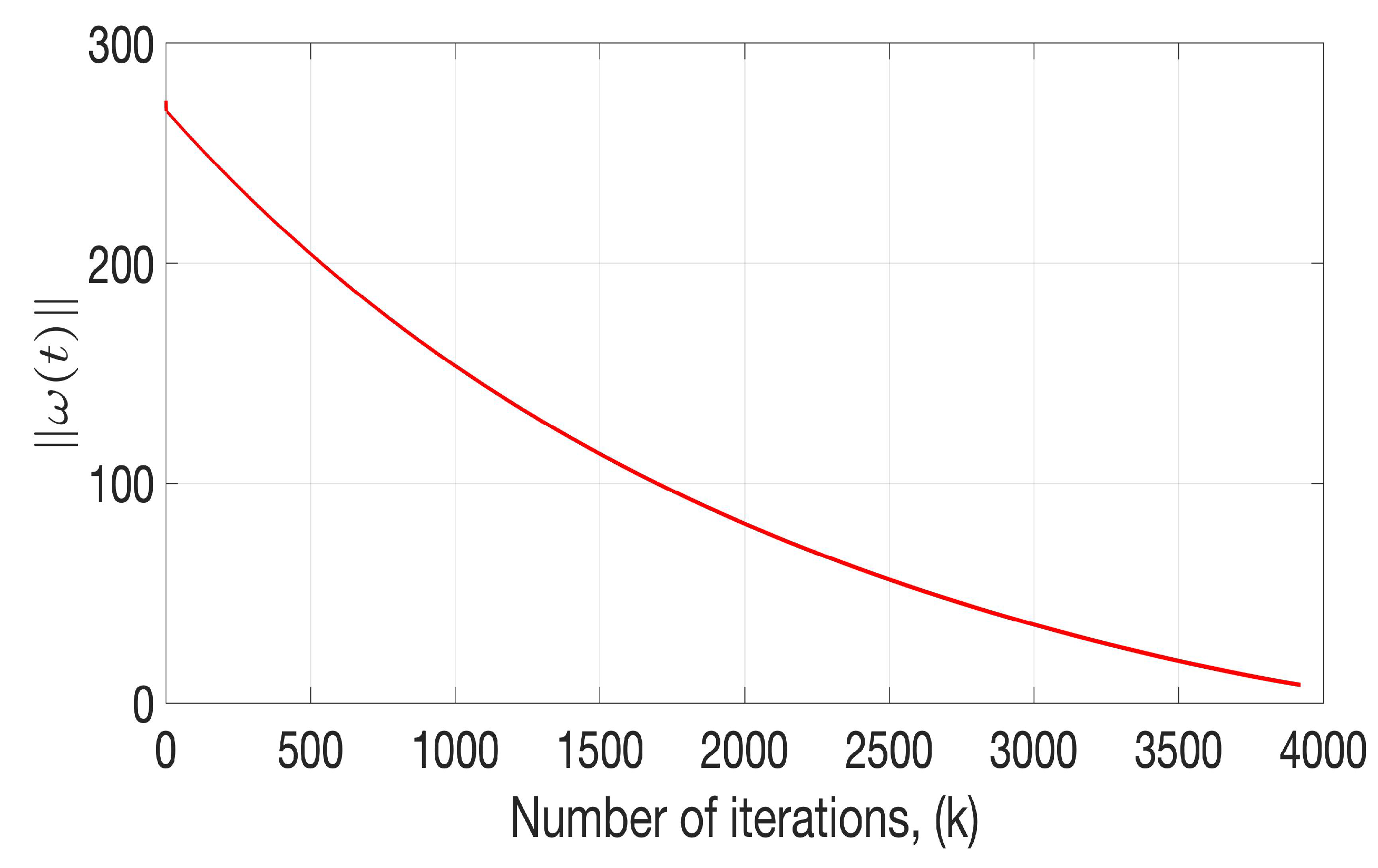
Noticing the dependence of the functional J concerning the weights, Figure 5 shows the evolution of the norm of the weights ${\omega }_K$ at the initial condition as a function of time. This temporal evaluation confirmed the weight tendency towards the origin according to the application of the Kiefer–Wolfowitz method. Even though the optimization strategy is not enforcing that the norm of the initial conditions should move to the origin, the continuous dependence of the system trajectories for the control action motivates this behaviour.

Based on the trajectories produced for the state x and the corresponding control action $u,$ the proposed functional J was estimated using the Formula (4). According to the case considered above for the states and the control, the evolution of the norm of the weights concerning time is also evidenced in this study in Figure 6, which confirms the effect of the optimization algorithm on the norm of the weights that are also participating in the evolution of the function. The selected example presented in this section shows the details of how the proposed algorithm could be used on an arbitrary system. Such a condition permits to claim that the algorithm introduced in this study could work for some other systems with similar dynamical structure as the one used in the example.

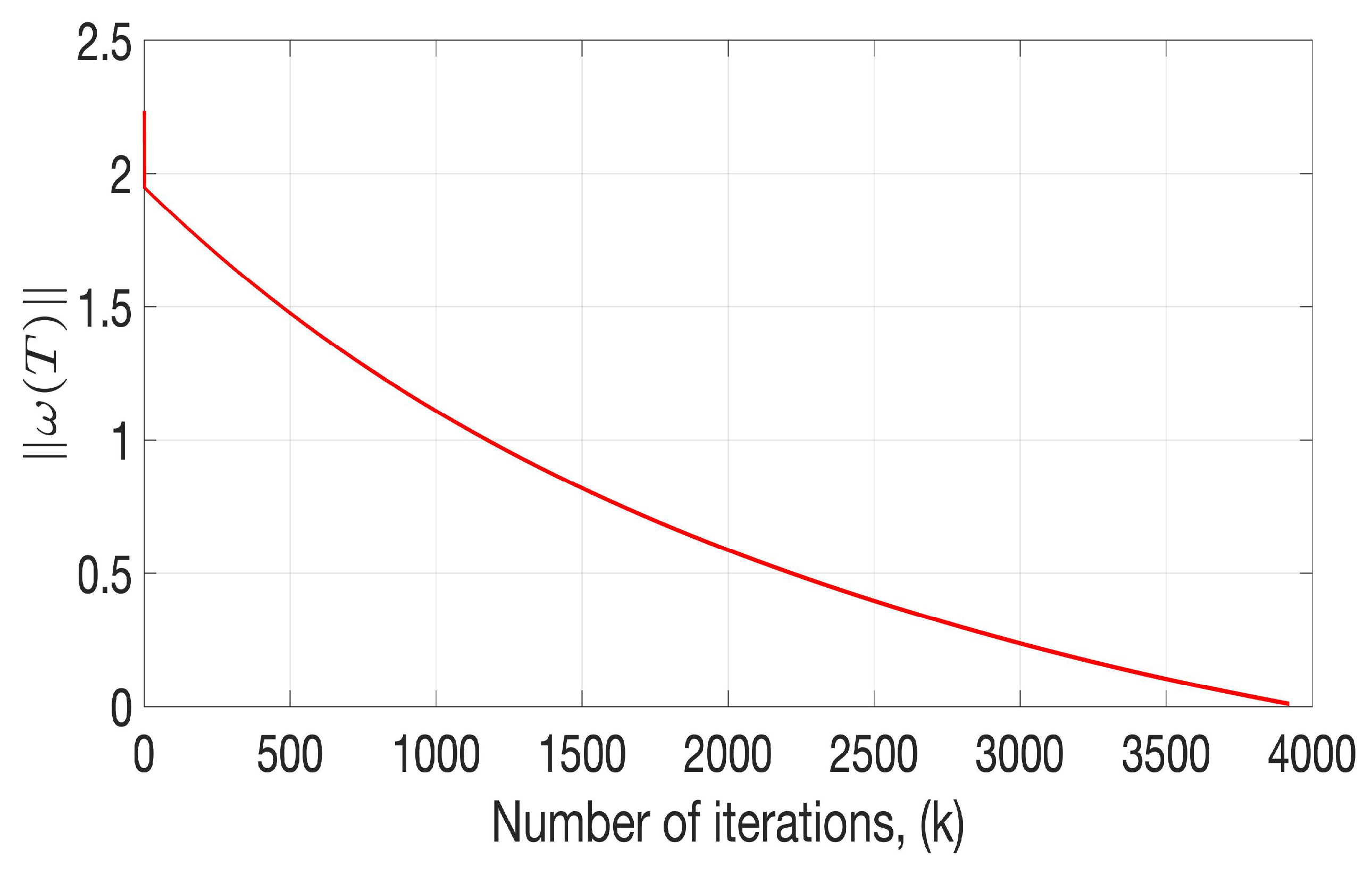
The evaluation of the Kiefer–Wolfowitz method allows for estimating the evolution of the norm for the final weights in the proposed DNN. The temporal evolution in discrete steps for the norm of these weights is shown in Figure 7. This evolution is shown along the entire set of iterations before the weights norm becomes smaller than 0.01, which is considered an early stopping criterion. As expected, the norm of the initial weights has a monotonically decreasing tendency to reach a final value of ${\omega }_{3900}\left(0\right)=0.01$. Because of the iterative algorithm is based on the evolution of the functional J at the final time T, the temporal evolution of this function over the iterations of the Kiefer–Wolfowitz method confirms the successful application of the recurrent optimization methodology.

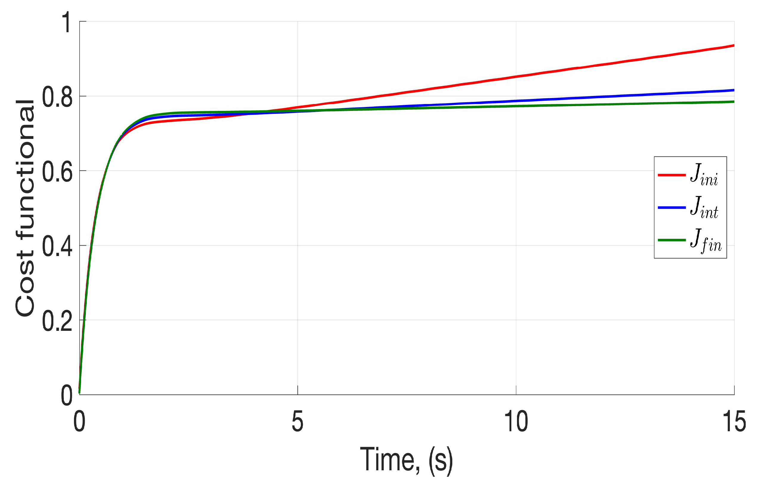
The application of the recurrent Kiefer–Wolfowitz method also implied significant effects on the temporal evolution of the cost function over the continuous time within each step (Figure 8).

The lines shown in Figure 8 represent the evolution of the performance function J evaluated with the weights proposed at the beginning of the iterative simulation $k=0$ (red line), one generated when the iterative process was evaluated with $k=1900$ (the middle of the iterative sequence, blue line) and one corresponding to the case when the iterative process was evaluated with $k=3800$ corresponding to the end of the process (green line). This figure confirms the iterative process leads to reducing the final value of the performance function, showing a non-increasing behaviour with respect to the number of iterative cycles. These characteristics confirm the sub-optimal construction of the proposed controller.

The variation of the cost function starts at the first round of the recurrent sequence with a non-convergent behaviour after 15 seconds. When the recurrent algorithm moves to its 1900 step (in the middle of the detected maximum number of steps), the cost function does not grow as fast as the case observed in the first step. When the recurrent algorithm reaches the last step, the cost function converges to an almost constant value of 0.8, which indirectly confirms the state convergence to the origin. Moreover, this final value obtained at the temporal evolution of the cost function within each stage of the recurrent algorithm confirms the observed result shown previously. Notice that this asymptotic behaviour of the performance function at the last step of the iteration algorithm is forced by the robustness of the developed controller to the class of admissible perturbations and modelling uncertainties.

9. Conclusions

The following are the main conclusions of this study:

This study provides a robust optimal controller for a class of perturbed non-linear systems using an approximate model of Bellman’s function based on a DNN formulation. The approximation of the min–max value function for the HJB equation allows developing the robust optimal control for non-linear systems affected by non-measurable uncertainties and perturbations. The analytical representation of the system trajectories $x^{*}\left(t\right)$ under the worst admissible uncertainties and perturbations ${\nu }^{*}\left(t\right)$ is obtained. The analysis of the HJB equation using the trajectories $x^{*}\left(t\right)$ and the approximated value function leads to deriving the learning laws for the DNN weights. The numerical procedure for adjusting the initial value of the weight dynamics is developed based on the modified deterministic version of the Kiefer–Wolfowitz method. The evaluated numerical example confirms the workability of the proposedrobust optimal control for a wide class of non-linear systems with an uncertain mathematical model.