Article

Modification of Learning Ratio and Drop-Out for Stochastic Gradient Descendant Algorithm

by
Adrian Teso-Fz-Betoño
1,
Ekaitz Zulueta
1,*,
Mireya Cabezas-Olivenza
1,
Unai Fernandez-Gamiz
2 and
Carlos Botana-M-Ibarreta
1
1
System Engineering and Automation Control Department, University of the Basque Country (UPV/EHU), Nieves Cano, 12, 01006 Vitoria-Gasteiz, Spain
2
Department of Nuclear and Fluid Mechanics, University of the Basque Country (UPV/EHU), 01006 Vitoria-Gasteiz, Spain
*
Author to whom correspondence should be addressed.
Mathematics 2023, 11(5), 1183; https://doi.org/10.3390/math11051183
Submission received: 25 January 2023 / Revised: 23 February 2023 / Accepted: 25 February 2023 / Published: 28 February 2023

Abstract

:
The stochastic gradient descendant algorithm is one of the most popular neural network training algorithms. Many authors have contributed to modifying or adapting its shape and parametrizations in order to improve its performance. In this paper, the authors propose two modifications on this algorithm that can result in a better performance without increasing significantly the computational and time resources needed. The first one is a dynamic learning ratio depending on the network layer where it is applied, and the second one is a dynamic drop-out that decreases through the epochs of training. These techniques have been tested against different benchmark function to see their effect on the learning process. The obtained results show that the application of these techniques improves the performance of the learning of the neural network, especially when they are used together.
MSC:
37M05; 37M10; 37M15; 37M20; 37M21; 37M22

1. Introduction

The stochastic gradient descendant algorithm [1] (SGD) is one of the most popular training algorithms for the multi-layer neural networks based on fully connected layers [2,3,4,5,6,7]. It is used as a quick learning algorithm based on its random behavior to reach a zone near the minimum loss quicker than other gradient-based algorithms. Its major virtue is also its weakness, as it will not stop naturally in the absolute minimum but will keep moving around that point constantly [7].
To avoid an unstable behavior of the algorithm, a learning ratio, also known as α, is applied to the gradient modification caused by the last loss calculated pattern for a certain synaptic weight; if α is set too high, the instability can have an effect on the training stability and ruin any progress on it. As for the error propagation from the output to the input in a supervised training, the deeper a weight is located, the closer it is to the input than to the output, and the less correction it will receive. This is caused because the gradient of the error will be vanishing while it is propagated through the layers, and the error portion that arrives to correct the deeper areas of a network could not be enough to have a powerful influence on it, needing more epochs of training to be able to move these deep weights. If α is set too low, this problem could be exacerbated. Generally speaking, α is set when the parameters of the learning algorithm are defined before the training of the neural network (NN) and are not varied in any point of the training. If the α set is too big, the synaptic weights can be modified in an instable manner, as the gradients are applied without any filter. This affects mainly the output-side weights, where the gradients have not been nearly vanished. On the contrary, if it is too low, the deeper synaptic weights will remain stationary as the gradient will not have any influence on them. The previous knowledge of the network designer and trainer is the one that determines the correct value for this parameter, and the whole training repetition could be caused in case a wrong value has been set.
On the other side, to avoid overfitting of the network, usually a drop-out [7,8,9,10,11,12] method is applied. This method consists of leaving apart, in a random way, some of the corrections caused by the gradients in the synaptic weights. This leaving apart makes the correction of a certain weight not complete, which in the course of the whole training allows a better generalization of the learned objective function. In a similar way to the learning ratio, a too big drop-out percentage will cause the network not to learn enough information from the training patterns, and if it is too low, there is a quite high risk of overfitting the network in the case where the training patterns bunch is not big enough or too many training epochs are set. As in the previous case, the network designer and trainer’s previous experience in NN training will be key to ensuring its correct use.
There are some major SGD modifications, such as the ones based on the AdaGrad algorithm proposed by Duchi et al. [13], where the observed data geometry is applied to the learning process, assigning frequent features lower learning rates and assigning higher rates to the infrequent ones. Since its publication in 2011, it has been modified in different areas to satisfy the special needs of each of them [14,15,16,17,18,19]. One of AdaGrad’s most important modifications is the RMSProp algorithm, solving the previous weaknesses found on it [20,21,22,23,24,25]. There are also other learning methods for the NN that give more precise learning ratios, such as the Levenberg–Marquard algorithm [26,27,28,29,30,31,32,33]. This method gives good results on the system loss but requires a high consumption of time and computational resources that could result in the training process not easily handling even the simplest problems.
The authors worked from the standard SGD, analyzing it thoroughly using the vectors scalar product between the generated ( L o s s W ) matrixes for each of the learned patterns and the average of them. To do so, the authors have developed a Matlab library to generate the neural networks and analyze them in detail by performing their own NN implementation instead of using the standard one from Matlab itself [34]. The library is able to collect data from each of the patterns. In the final epoch of training, the data of all the weight matrixes of the created neural network are stored and processed. The main reason for creating this library is to be able to collect all these data that are not offered by other NN libraries such as Keras or Matlab in order to be able to manipulate the learning algorithms and take out the needed graphical charts to study the behavior of the NN. This way, it is possible to analyze the impact of the modifications on the behavior of each of the learning patterns and seen if there is any change in them. The chosen specter of math functions to be the target functions for the shallow NN used for the experiments offer a graphical way to see if any of the modifications have effects on them and detect any malfunction during training as a problem of the learning process instead of a randomness of the training objective.
In this paper, the authors propose a modification in the learning ratio and the learning drop-out, making them dynamic to obtain a better convergence in a similar time. This way, the need for an experienced hand on the NN training is made less determinant for the final result. The proposed modifications are complementary to the authors’ previous works on the SGD and drop-out modifications. The authors’ goal is to achieve some better results on the learning process without sacrificing time and computational resources in the process, being able to make the NN learn better in an inexpensive way.
The paper is organized as follows. First, in Section 2, a background on the SGD modifications made by other authors is analyzed, where some performance improvements are displayed. In Section 3, the studied learning ratio and drop-out issues are analyzed, and modifications for a possible solution are explained. In Section 4, the performed experiments are displayed as well as the obtained results. Section 5 contains the conclusion; and, finally, in Section 6, the possible future lines of work are listed.

2. Background

As said before, the SGD is a very popular training algorithm but suffers from various weaknesses regarding the training process. Different authors have proposed different kinds of modifications. Le Roux et al. [35] and Defazio et al. [36] propose a modification on the algorithm by adding a memory of the past gradients to use the average of it in the first case and, in the second case, being an evolution of the first, an incremental gradient modification. In both cases, they claim to obtain quicker convergence than the standard algorithm. Following a similar approach, Johnson and Zang [37] propose a modification to use a predictive variance reduction for the SGD achieving also a quick convergence on the minimum Loss. Zhuang Yang [38] proposes combining a conjugate gradient algorithm with a stochastic recursive gradient descendent algorithm to take advantage of both the convergence quickness of the first one and the relative direct way of step shaping of the second one to achieve a reasonable convergence in a reasonable computational time. Similarly, Pengfei Wang and Nenggan Zenhg [39] propose two methods to achieve a linear convergence to the minimal solution by using an asynchronous stochastic recursive gradient. Li et al. [40] propose a modification of the stochastic parallel gradient descendant algorithm for the free-space optical communication. Their adaptation follows the work originally made by Hu et al. [41] for fiber coupling. Their adaptation consists of feeding the loss feedback with multiple data instead of the loss generated in a single pattern. Le Trieu Phong and Tran Thi Phoung [42] propose another modification of the SGD by adding compression and memorization of the gradient to achieve more accuracy and less noise during the NN training. From a safety and security point of view, Roberts and Smith [43] propose a simplified convergence theory, which was originally presented by Blanchard et al. [44] to modify the SGD and make it resilient to the Byzantine type of attacks in distributed learning.
There are also authors using the SGD algorithm as a basis for other modifications and experiments. Chen et al. [45] extensively studied the SGD’s behavior during the training and travel through the loss landscape. They concluded that the SGD algorithm has a super-diffusion behavior on the initial steps of the training, allowing it to travel fast from the rough fractal-like loss regions to the flattened, nearly minimal loss regions; once the training process advances, however, the behavior changes to sub-diffusive, which allows the grain approach to the minimal loss region once the landscape has become more flat. They analyzed also the different hyper-parameters of the SGD algorithm and their influence on the training of the NN. In the same terms, Carmina Fjellström and Kaj Nyström [46] made a diffusion map out of the different elements that compound the SGD learning and the loss surface. Sun et al. [6] analyzed the effect of using computer floating numbers instead of continuous ones in the SGD algorithm and see effects such as overflows on it. In the neural trees world, Varun Ojha and Giuseppe Nicosia [47] modified a neural tree to shape it like a single neuron neural tree trained using SGD. Senthil et al. [48] developed an SGD-based algorithm named Aladelta SGD to be able to store the data from hospital patients in the most time and space-efficient manner. This way, predictions on diseases can be more easily achieved.
In the case of the drop-out technique, adaptative drop-out techniques are widely used. Lei Jimmy Ba and Brendan Frey [49] proposed one of the firsts adaptative drop-outs, decreasing considerably the loss obtained compared to the standard drop-out. Li et al. [50] propose an adaptative drop-out based on biological principles of the gene theory and human brain neurons. They claim to obtain an adaptative drop-out that can improve the feature extraction performance and the classification accuracy. Mirzadeh et al. [51] studied the relation between the drop-out and the continuous training of a network; they are able to demonstrate that the NN that incorporates drop-out in their training algorithm is more stable, maintaining an old learned task while learning new ones. Yuanyuan Chen and Zhang Yi [52] propose an adaptative sparse drop-out technique that trains a few neurons in each layer, obtaining them in a probabilistic method based on a sigmoid function. Daniel LeJeune et al. [53] also propose another adaptative drop-out approach, the effective penalty Ω, having good results on sparsening approaches.

3. Learning Ratio and Learning Drop-Out: Issues, Analysis and Possible Solutions

The authors propose two main improvements in order to achieve better results in training algorithms. The first one is the dynamic learning ratio that depends on the position of the layer inside in the neural network. The second is a dynamic drop-out that adapts the drop-out probability among the epochs of training. The main objective of these two improvements is to reduce the loss function achieved with the training algorithm without increasing the training time. The authors have tested these two improvements on their own and together. These possibilities have been tested in order to see the influence of each improvement.

3.1. Dynamic Alpha

This improvement consists of applying an adaptive layer-wise learning ratio. This adaptive policy increases the learning ratio in the same epochs if the weight is located in a layer closer to the input. The authors have noticed that the training algorithm in SGD propagates the error through the output to the input, and that delays the training process of weights that are closer to the input layer. So, the weights that are closer to the input learn slower than the weights that are closer to the output. In order to increase the actualization of whole weights in a more homogeneous way, the authors propose a bigger learning ratio in weights that are closer to the input. In Equations (1)–(4), the authors define the training equations applied in this research work. w i , j , n ( t ) is the weight that links the j-th output to i-th input of the n-th layer, mi,j,n(t) is the momentum applied to that weight and ( L o s s w i , j , n ( t ) ) is the partial derivative of the loss for that particular weight. α and β are the learning ratio, the one to be adapted, and the momentum appliance ratio. The authors propose in Equation (4) a modification that introduces an adaptive term. This term depends on n, N l a y e r s , ξ   and α 0 parameters. The ξ   parameter is the learning ratio’s increased value for the whole neural network.
w i , j , n ( t + 1 ) = w i , j , n ( t ) + Δ w i , j , n ( t )
Δ w i , j , n ( t ) = α ( L o s s w i , j , n ( t ) ) + β m i , j , n ( t )
m i , j , n ( t + 1 ) = m i , j , n ( t ) + Δ w i , j , n ( t )
α = α 0 ( 1 + ξ n N l a y e r s )
The authors remind the reader that this improvement has been implemented because the error propagates from output to input. Thus, the error vanishes when it propagates from the output layer to the input layer in the SGD training algorithm. The n index is equal to 0 for the output layer weights and n is equal to N l a y e r s . This term (see Equation (4)) tries to increase the actualization of weights that are closer to the input.

3.2. Dynamic Drop-Out

The drop-out is a very well-known regularization technique. This technique equals to zero an activation in a random way with P d r o p o u t probability. This probability usually is a constant value for fully connected layers. The authors propose that this probability must be adaptative in order to modulate its influence along the training epochs.
P d r o p o u t = P d r o p o u t , 0 e t T
This adaptive probability allows the training algorithm to introduce a faster specialization of each neuron at the initial epochs of the training. In that way, the training algorithm allows neurons to learn a specific pattern or feature faster. In the start, the neurons of the same layer have the same probability to acquire the most important features. There are several training epochs after the neurons obtain their specific feature or learned pattern. In order to promote this specialization, the authors propose an adaptive or dynamic probability of drop-out. In Equation (5), the authors propose an exponential shape function, where the vanishing coefficient is T. If this vanishing term must be bigger, this T parameter must be increased. The P d r o p o u t , 0 probaility is the initial drop-out probability.

4. Shallow Neural Network Examples and Results

Based on the authors’ previous work, some experiments were made using Matlab 2022a as the development tool. The authors use a shallow neural network composed of three fully connected layers separated by two ReLu processing layers. The training function will be MSE. All three fully connected layers are trained using 0.01 α and β values and a 20% of drop-out rate. Each of the experiments has been made using the standard SGD parameters to have a reference of the learning ratios that can be obtained normally and applying the modification techniques. The authors have applied this kind of neural network because conceptually, in shallow neural networks, the regularization effects are less important than in deeper neural networks. So, if the authors obtain goods results in such shallow neural networks, the benefits must be bigger in very deep neural networks. The experiments consist of 6241 patterns of learning and 3136 patterns of validation that are learned in 100 epochs of training. Both data sets have been generated stochastically inside the data set bound to each of the benchmark examples. The chosen benchmark functions make it easy enough to trace any problem in the training to the learning process itself and not to any other complex side effects. The obtained output results are based on the behavior of the different training patterns compared to the average behavior. These comparisons are represented by the scalar product between the partial derivative of a pattern loss to a certain layer ( L o s s W ) and the average one, obtaining j × i weight matrixes in the fully connected layers. Those matrixes are transformed into a single row vector, ordering them from output to input and making the scalar product. The shown modules relationship and cos(φ) are the result of those products.

4.1. “Mexican Hat”

This mathematical function is what the authors have used as a starting point of analysis against the different studied possibilities of mutation of the SGD algorithm. The equation leading this function is the following one:
z = s i n c ( x 2 + y 2 ) ; x , y     [ 0.95 ,   1 ] ,
where x and y are the inputs for the neural network and z is the expected output. We first train the network without applying any of the techniques proposed in this work to have a starting point for comparison.
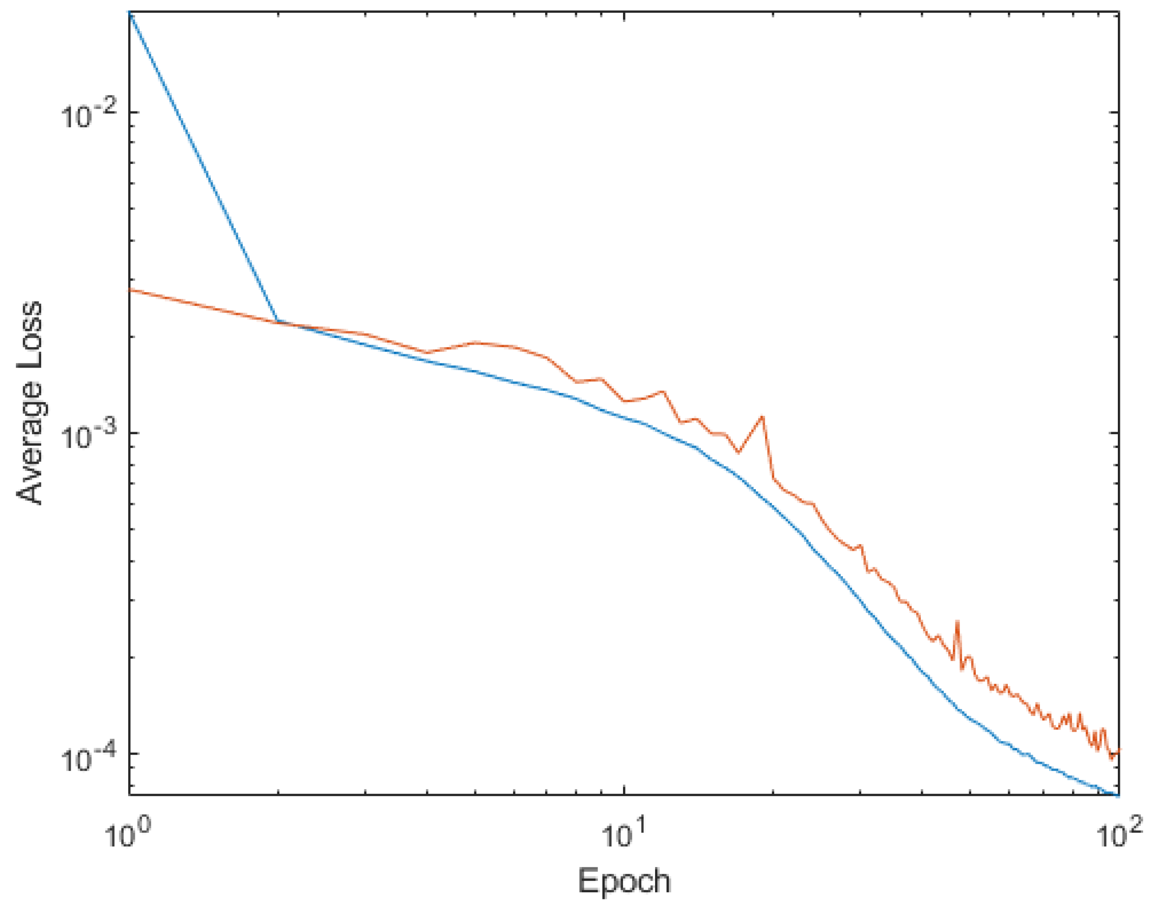
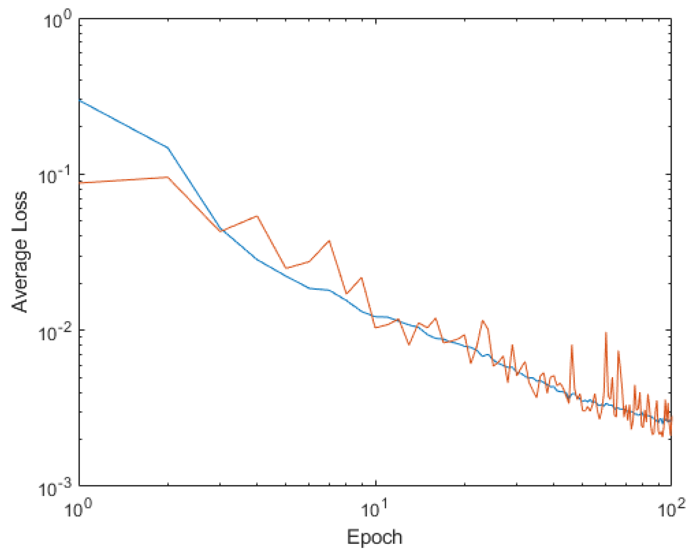
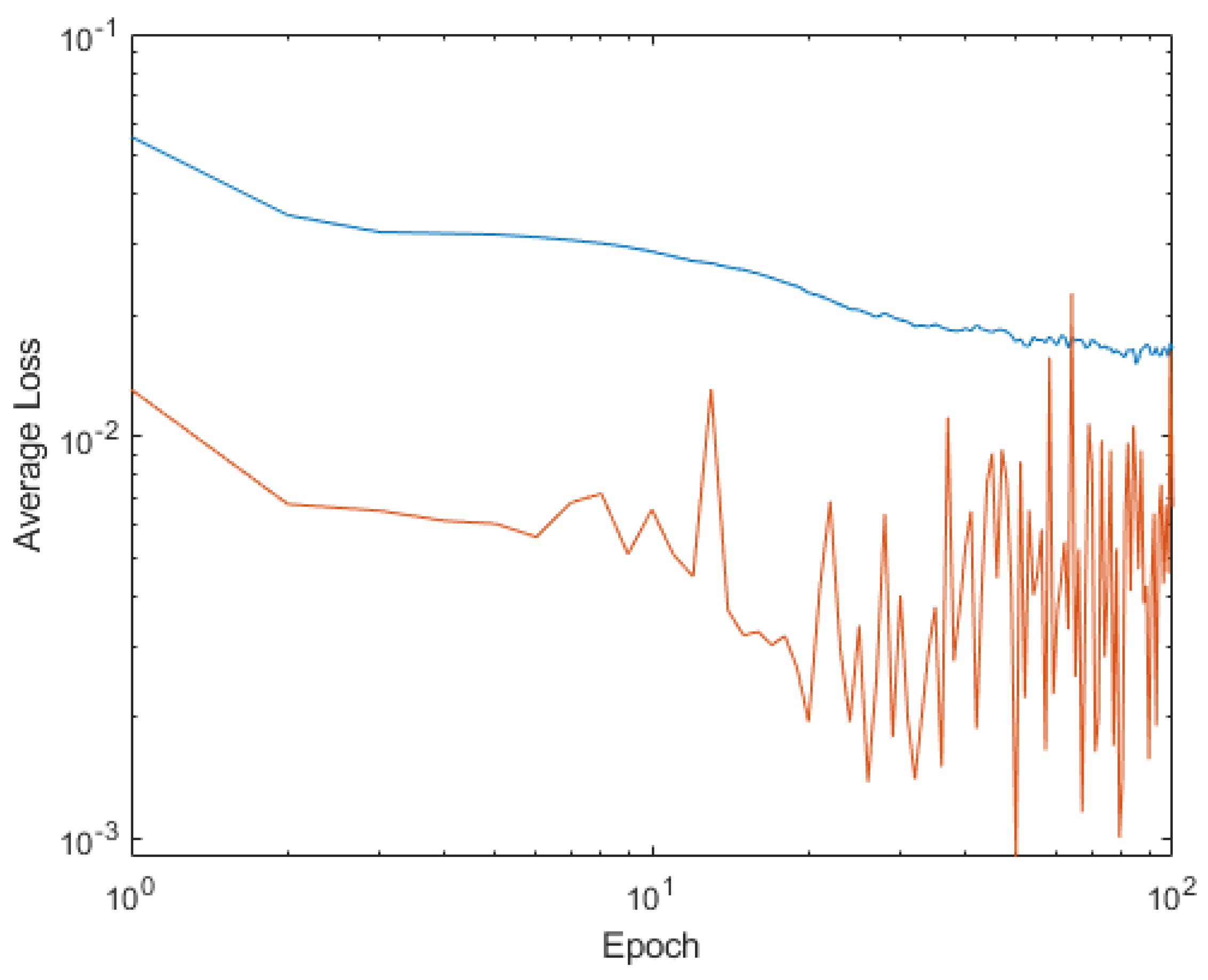
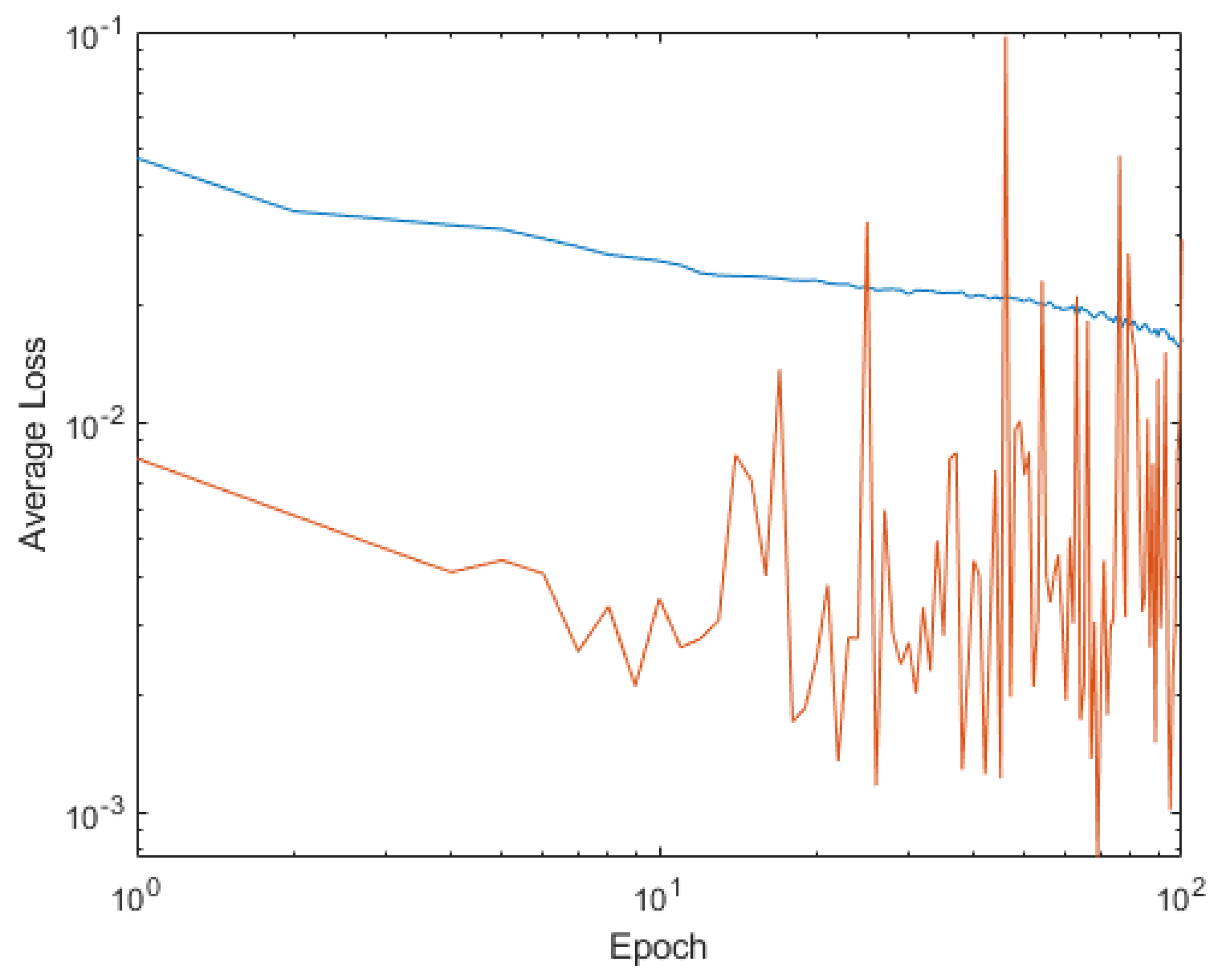
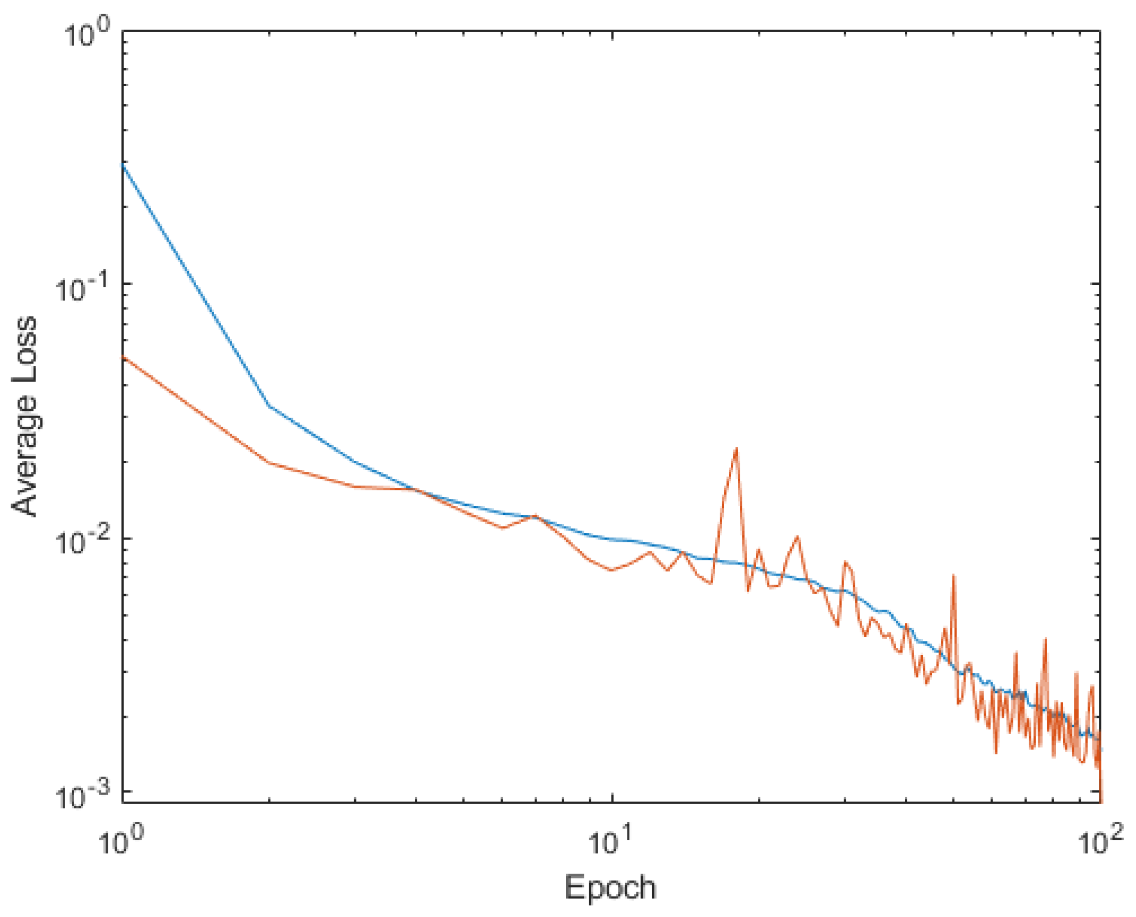
On this particular case, after all the training is completed, the average loss of training patterns rises to 0.00010586 on the learned patterns and 0.000150754 on the case of the validation patterns at the end of the 100th epoch of training. Figure 1 shows the evolution of the training loss on a logarithmical scale. The authors will compare this obtained value with the ones obtained applying the modifications proposed in this work.

4.1.1. Dynamic Alpha

Applying the dynamic alpha modification, see Section 3.1, and training the same neural network with the same patterns, through the same number of epochs, the obtained average loss is 0.000073996 in the case of the training patterns and 0.000104274 in the case of the validation patterns. In Figure 2, the evolution of the loss during epochs can be seen.
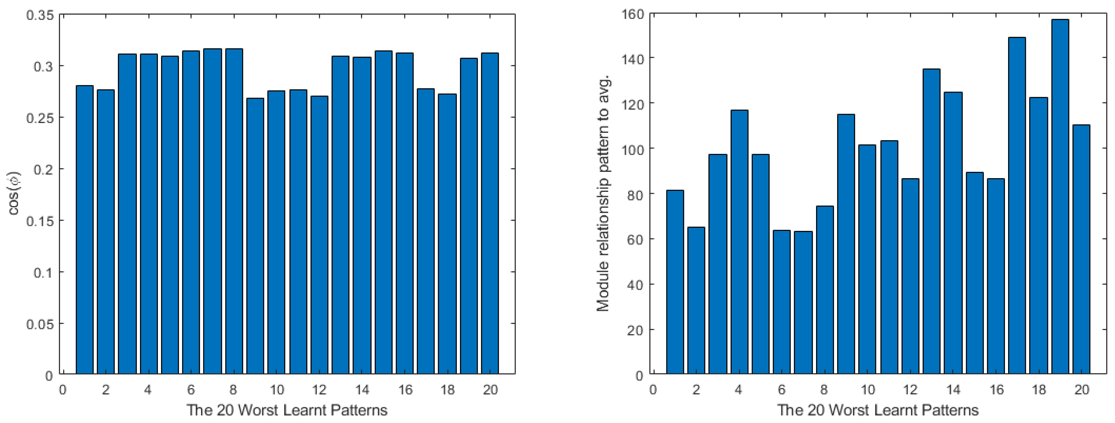
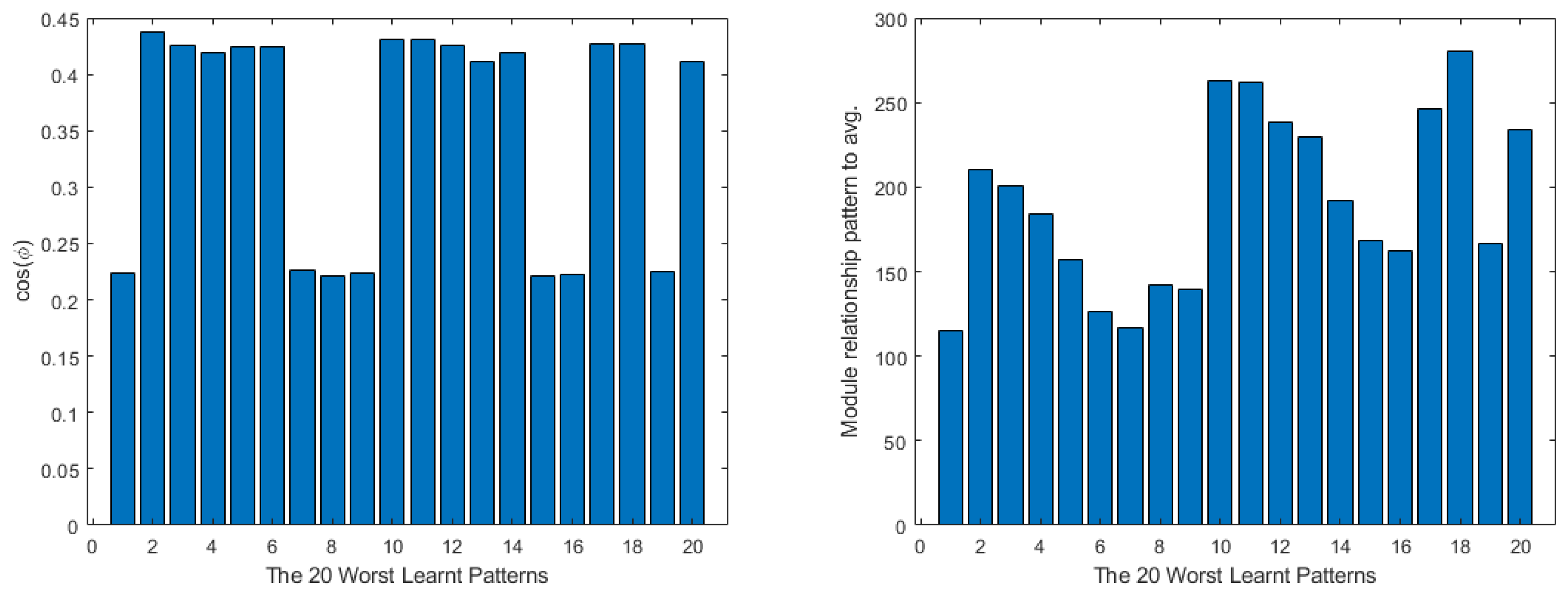
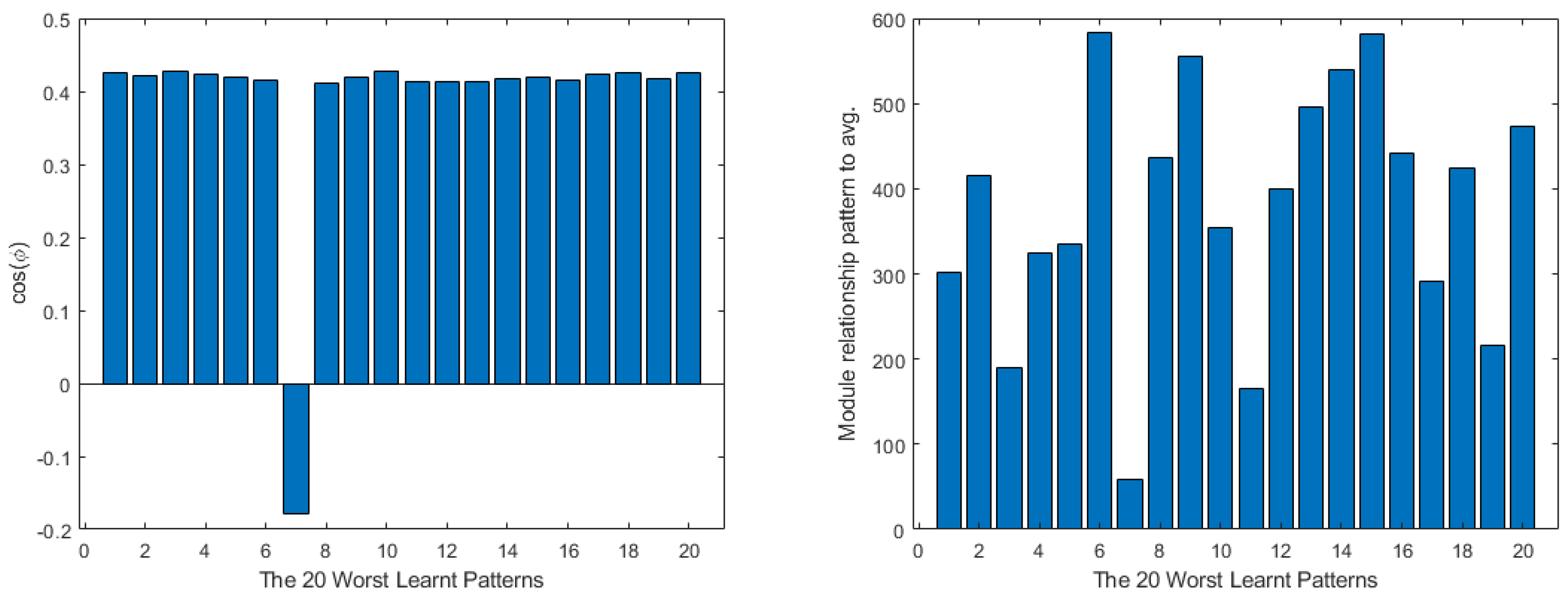
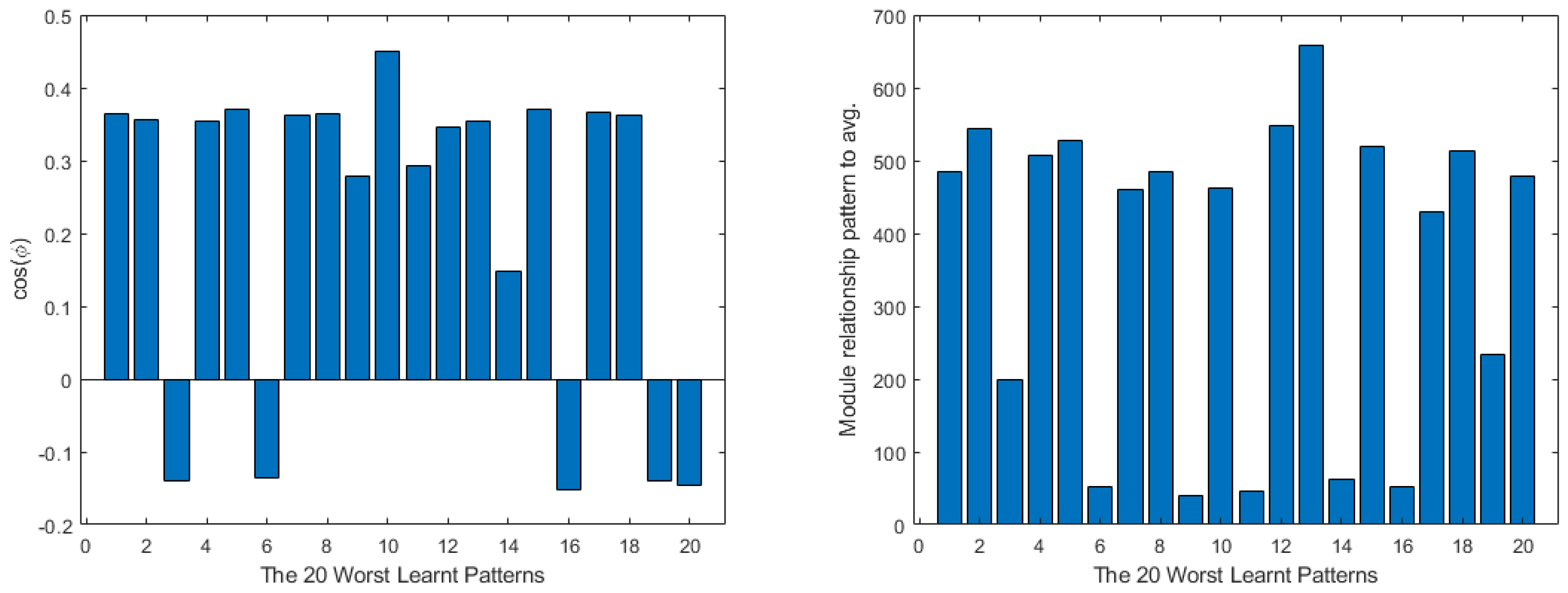
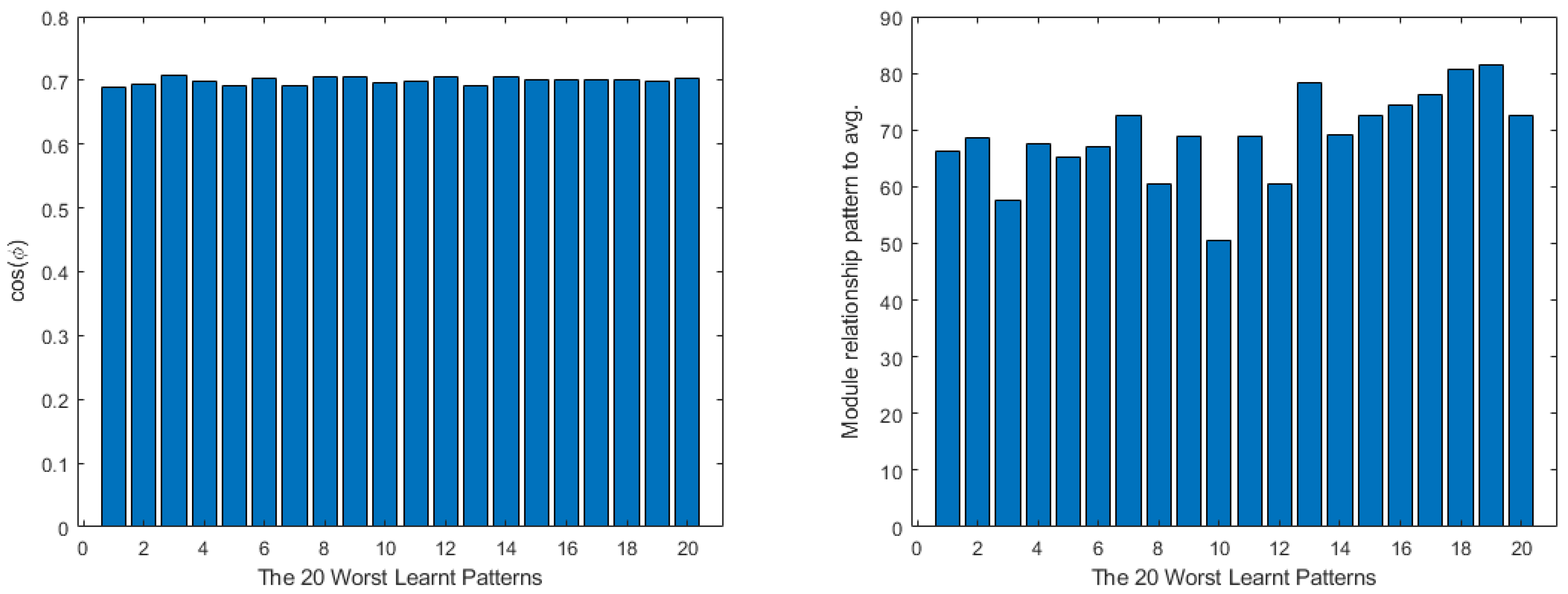
The authors used the previous work to propose patterns of vectors alignment [34], using the scalar product method between each of the patterns and the average of all the patterns. The 20 worst learned patters are barely aligned with the average of the network, as their cos(φ) values are below 0.5 and their module values are much bigger than the average vector. In Figure 3 is possible to see this effect.
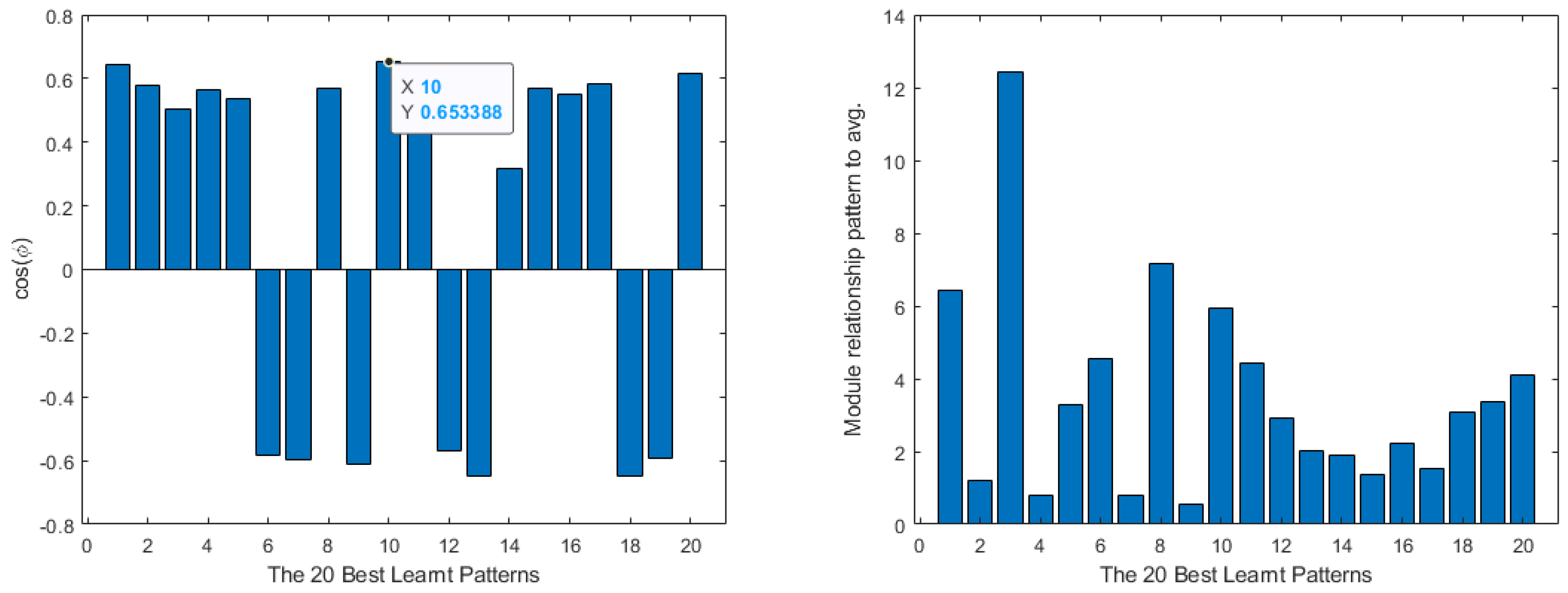
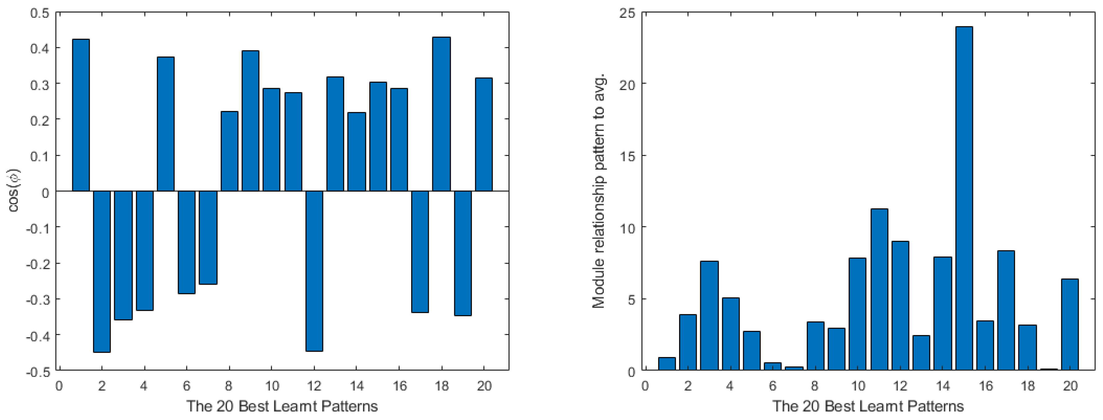
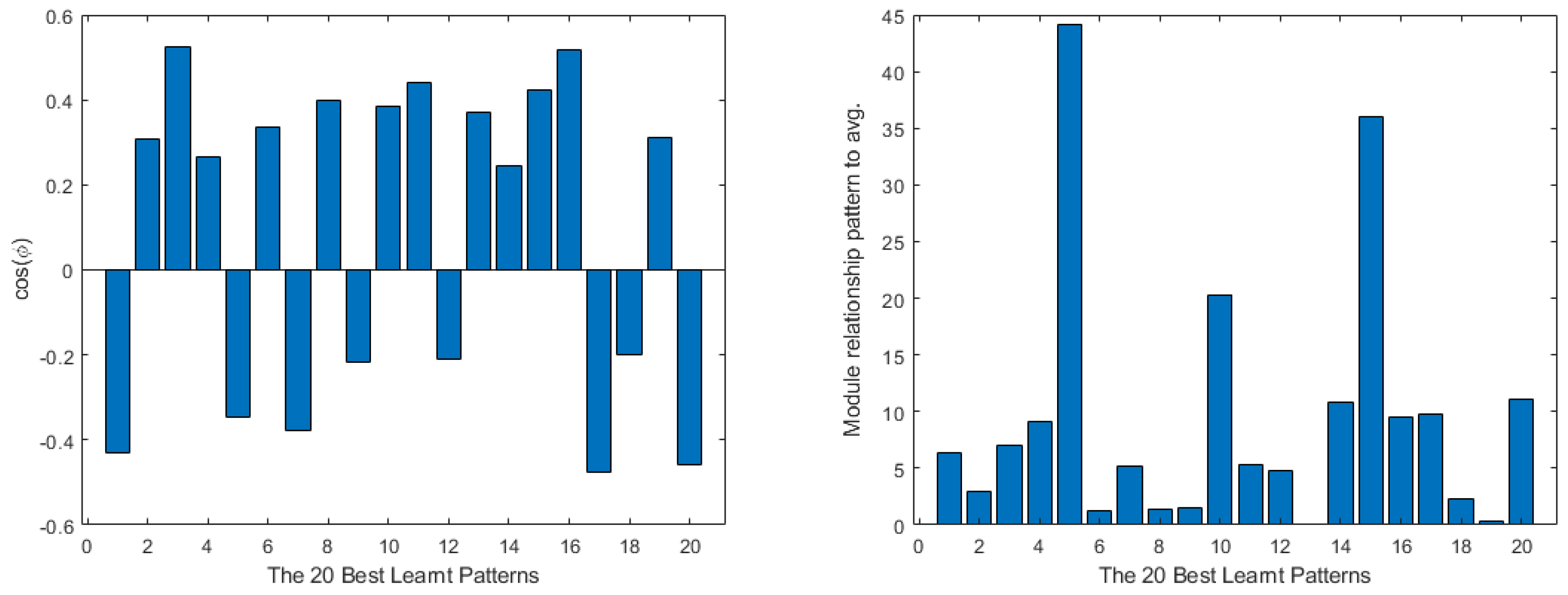
On the opposite side, the 20 best learned patterns show a much more aligned situation to the average vector. The module relationship, instead, is much smaller than the case of worst learned patterns, with some even being close to a 1:1 relationship with the average value. Figure 4 shows these results.
In summary, for this particular case, it can be said that the dynamic alpha application to the learning process improves the learning ratios compared to the original SGD algorithm in this particular case. The best learned patterns have more presence in the learning of the network as they are very aligned to the average of the network, while the worst learned ones have nearly no presence in the final result, as they offer a nearly orthogonal response to the average of the network.

4.1.2. Dynamic Drop-Out

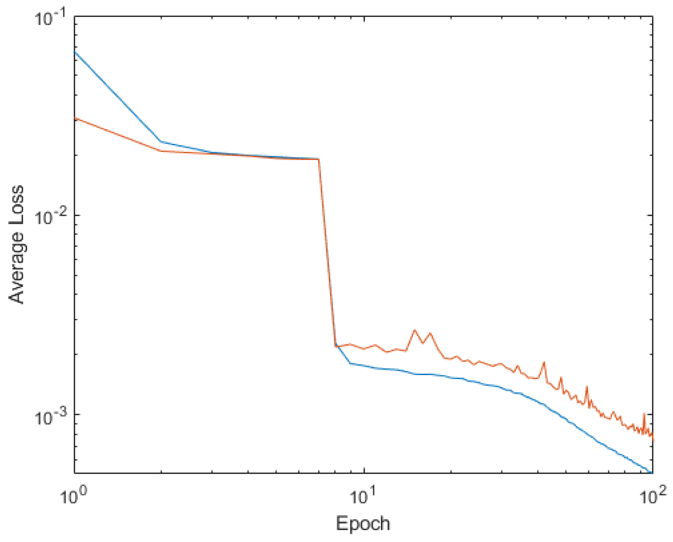
In the case of the of dynamic drop-out, see Section 3.2, the average loss of training patterns rises to 0.000248867, which is two times bigger than the original, and 0.000330196 for the validation patterns. The numbers were not promising, but still, the authors processed the obtained data from the training. Figure 5 shows the evolution of the loss.
The 20 worst learned patterns show a similar behavior to the dynamic alpha ones, which is a little more aligned but still having their cos(φ) below 0.5; the module relationship is also big, as the patterns modules are over 100 times bigger than the average. Figure 6 shows this behavior.
On the 20 best learned patterns side, the results are quite similar to the application of the dynamic alpha. The patterns are generally more aligned and their modules are much closer to the average value. In Figure 7, this behavior can be observed.

4.1.3. Mixed Together

Finally, another experiment was made combining both modifications at the same time. After the training, the average loss rose to 0.000076558 in training patterns and 0.000099538 in the validation ones. Figure 8 shows the evolution of these values through epochs of training. It can be seen that the loss reaches similar values to the case using only dynamic alpha, but the validation patterns loss is maintained closer to the training ones than in the previous case, being further from the overtraining.
These values are near the dynamic alpha, but analyzing the error on each of the validation points, on the combination method, the peak errors are much lower than in the first-case ones. In Figure 9, it is possible to see that the peak errors in the case of only using dynamic alpha are bigger those in than the case of using both dynamic techniques.
Analyzing the data obtained from the training, the authors see that the worst learned patterns are much more aligned with the average value, having their modules relationships closer to 1 than the cases before, and the cos(φ) are over 0.6 in absolute value. Figure 10 shows this behavior. These means that the worst learned patters are more relevant in the learning process and affect more weights in the fully connected layers.
In the case of the best learned cases, the behavior is similar to the previous cases. Figure 11 shows how it is similar to the dynamic alpha-only or dynamic drop-out-only cases. After seen the obtained results, it can be said that the combined methods make the network learn better than the case of standard SGD is used in the training, and they make all the patterns more relevant to the training process.
After checking that this effect was working on this particular case, the authors took some other benchmark functions from Surjanovic and Bingham’s web page [54] to check if the new discovered method has the same positive effect on the training.

4.2. Ackley Function

The Ackley function presents an absolute minimum in the [0,0] position and many local maximums and minimums around it. The following equation represents its form:
z = 20 ·   e ( 1 5 1 2 ( x 2 + y 2 ) ) e ( 1 2 ( c o s ( 2 π x ) + c o s ( 2 π y ) ) + 20 + e ;   x ,   y   [ 0.95 ,   1 ]
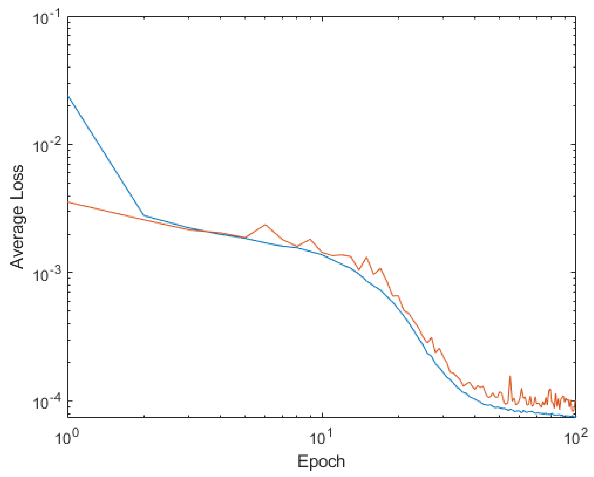
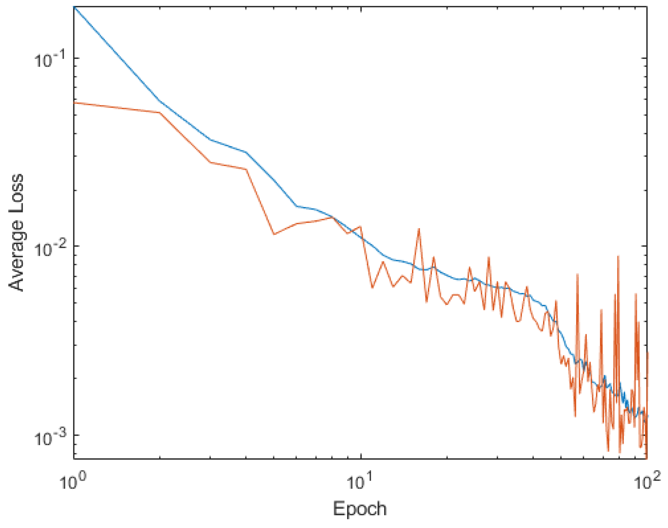
where x and y are the inputs of the neural network and z is its output. After the 100-epoch training without applying any modification to the SGD, a loss of 0.003114478 is obtained on the learning patterns and 0.002884209 on the validation patterns. Figure 12 shows the loss evolution through the epochs, and it can be seen that the loss associated with the validation patterns set becomes noisier in the final steps of learning.
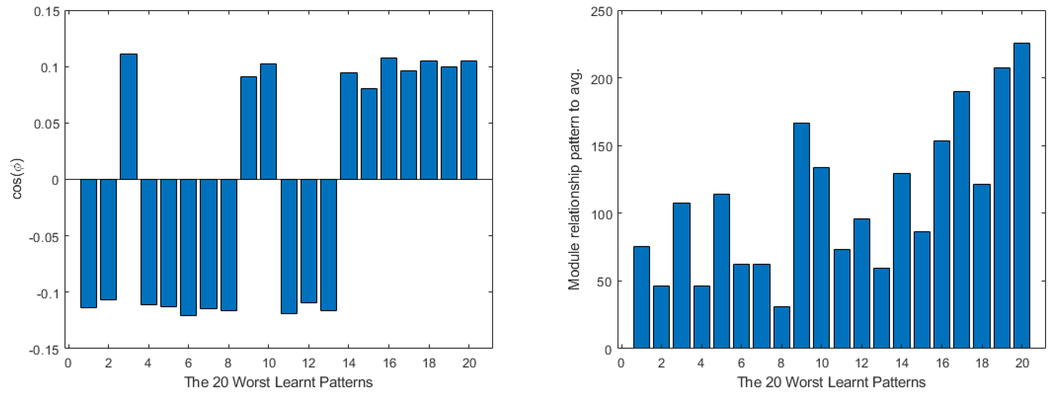
Viewing the data obtained from the learned patterns, the worst learned are barely aligned, and comparing their modules to the average calculated value produced values of over 200 in most of the cases. Figure 13 shows these data. In the case of the best learned patterns, the situation is similar to the one that was seen before, having a similar behavior in the cos(φ) but with a module relationship to the average that was much lower. Figure 14 displays these data.
After making the training with the dynamic alpha and drop-out, it is possible to see that the loss has been improved a bit in both cases, being 0.00250811 in the training patterns and 0.002813870 in the case of the validation patterns. Figure 15 shows the evolution of loss through epochs: the noisy part of the validation patterns is still there, but its effect has been reduced.
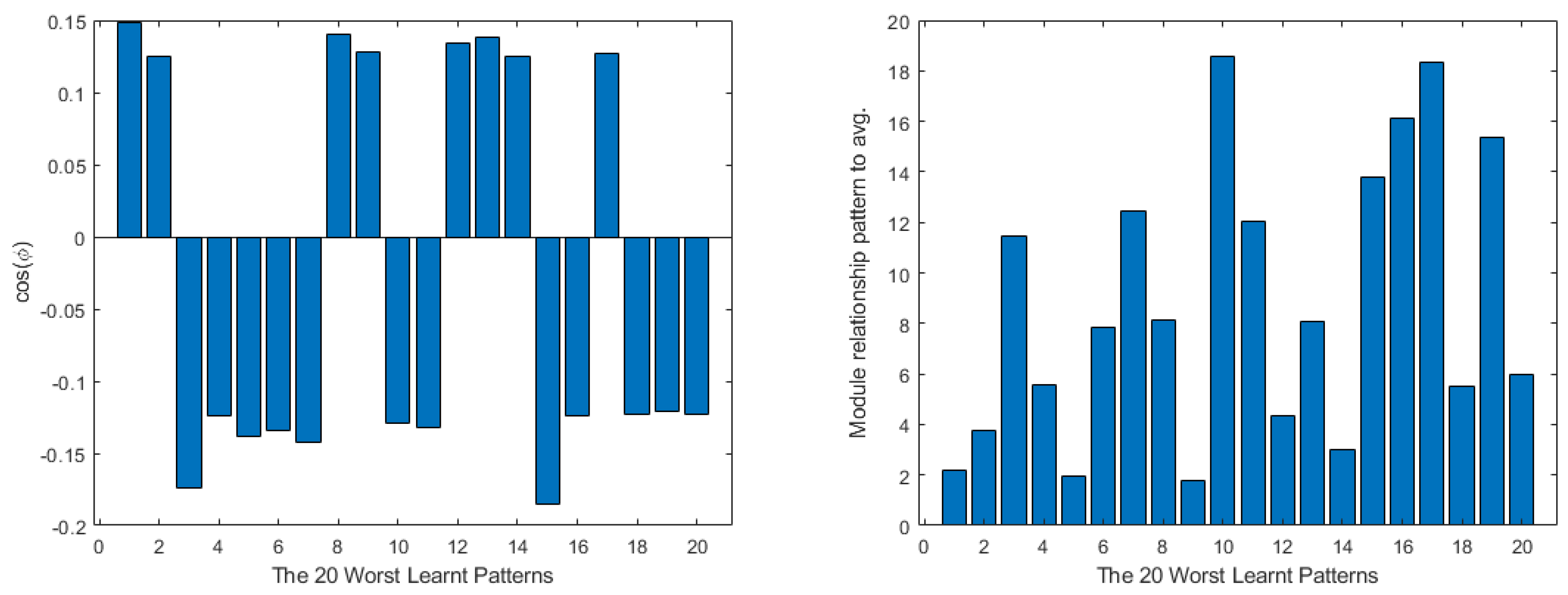
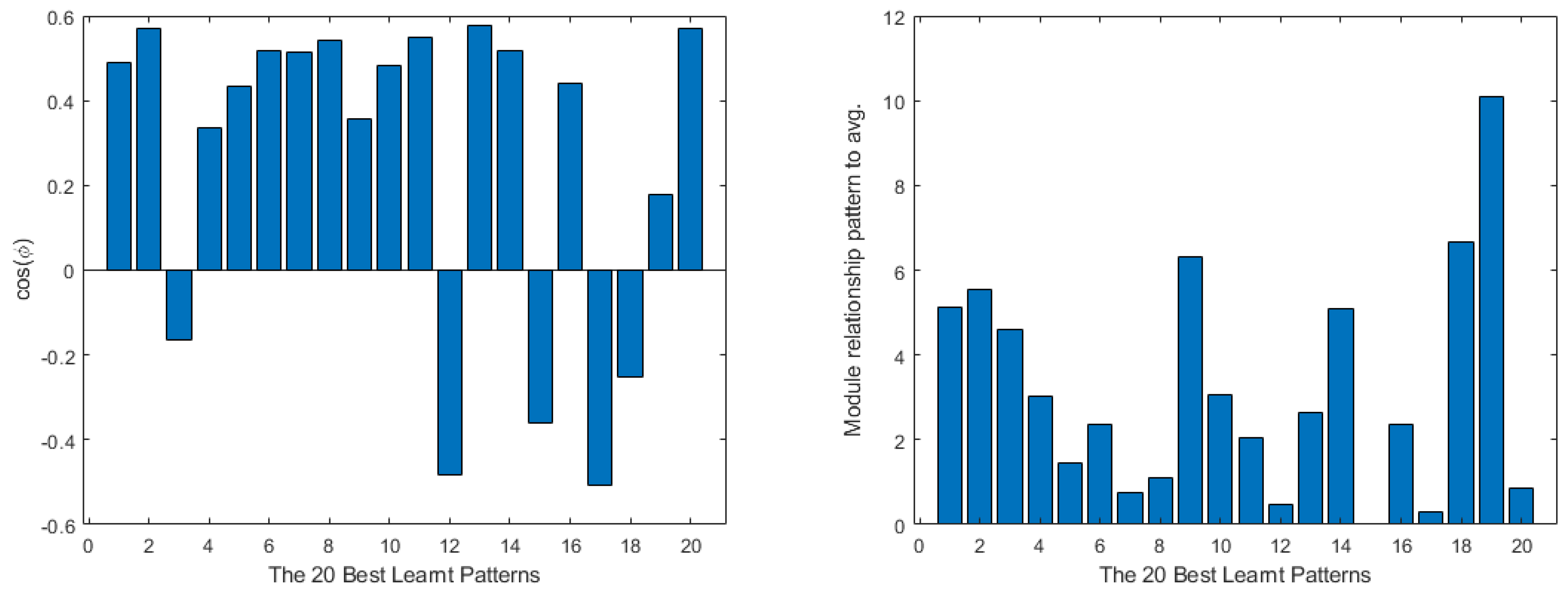
Analyzing the patterns, the worst learned ones have a similar behavior in the angle alignment as before, but the module relationship has been lowered significantly. Figure 16 shows the obtained values. In the case of the best learned patterns, the situation is quite similar: the cos(φ) remains quite similar while the module relationship has been lowered significantly; is possible to see in Figure 17. Overall, it can be said that the behavior of the patterns is closer to the average learning value than in the case without modifications.

4.3. Cross-in-Tray Function

On the case of the Cross-in-Tray function, the following equation intended to be achieved:
z = 0.0001 ( | s i n ( x ) s i n ( y ) e ( | 100 x 2 + y 2 π | ) | )   x ,   y   [ 0.95 ,   1 ]
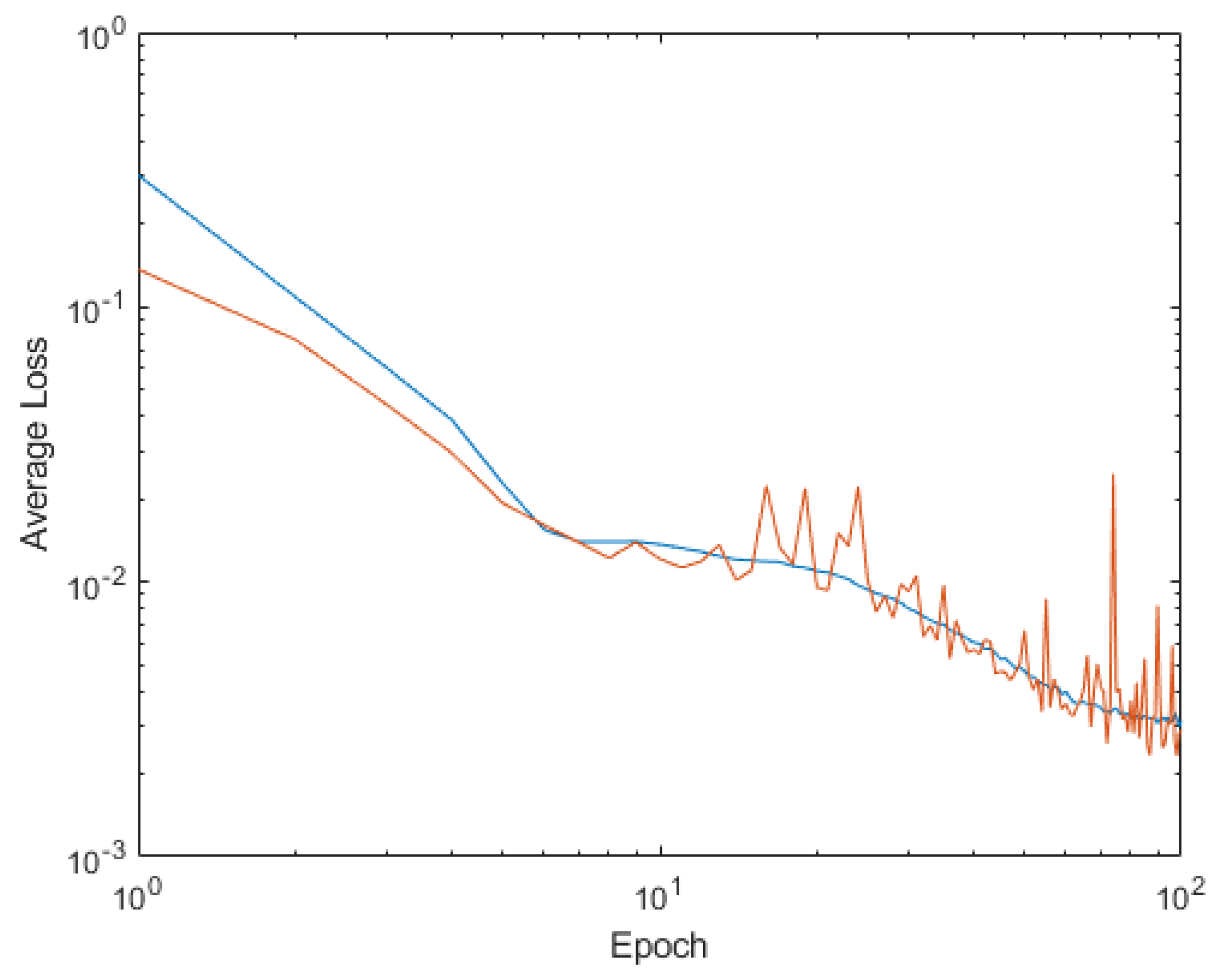
where z is the wanted output for the output and x and y are the inputs. After training the network with standard SGD and the one with dynamic alpha and drop-out, the obtained loss is 0.016488167 in the training patterns and 0.006663838 in the validating ones for the standard SGD. As it can be seen in Figure 18, the validation patterns loss has a quite random behavior during the training process: it is generally below the training loss, but does not have a clear process of learning. The learning parameters loss, instead, has a descendant tendency, finding probably a local minimum in the final steps of learning.
In the case where both modifications are applied, the loss reaches 0.016340295 for training patterns and 0.029352279 for the validating ones. The validation patterns’ related loss is as noisy as before, as can be seen in Figure 19.
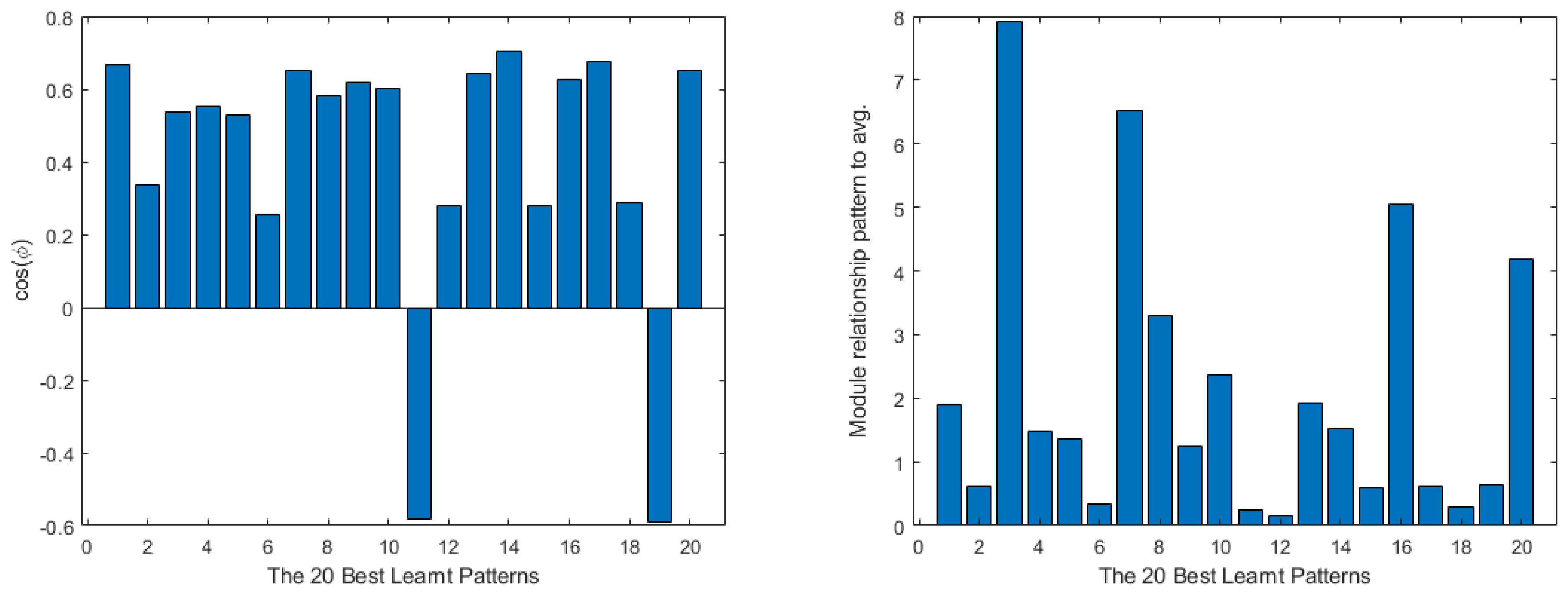
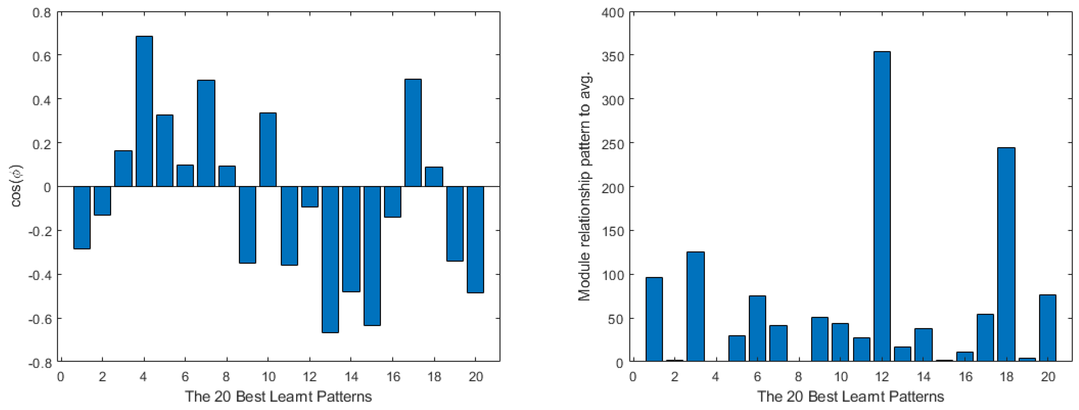
In this case, the differences are not very obvious between both cases. Analyzing the data obtained from the learned patterns, the worst learned ones present a negative cos(φ), which means that all these patterns are pulling the learning the training away from the average value. The modules’ relationships to the average are all over 100. These values can be seen in Figure 20. On the best learned patterns side, the cos(φ) is quite low, meaning that even the best learned ones are not very relevant to the training; this can be seen in Figure 21. Perhaps the network should be changed to fit better the function with this learning algorithm in its standard mode.
In the case of the modified alpha and drop-out, the worst learned patterns are mostly aligned with the average value, changing completely the direction of them, while the modules maintained high values, as can be seen in Figure 22. The best learned patterns, instead, maintain their behavior almost completely; see Figure 23. As said before, perhaps the network must be modified to be able to train correctly this particular case with the SGD algorithm.

4.4. Drop-Wave Function

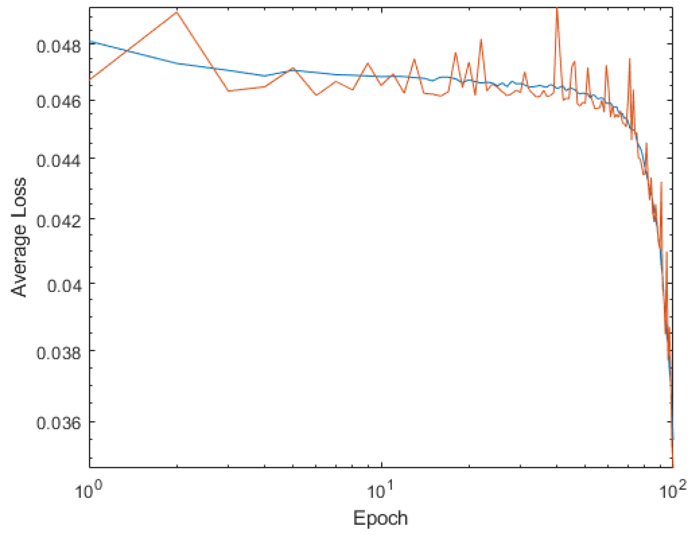
In the case of the drop-wave function, the obtained difference is quite significant, while the loss in the standard SGD reaches 0.035496386 and 0.034738452 in the validation patterns. Analyzing Figure 24, it is possible to see that the loss evolution happened primary at the final epochs of training.
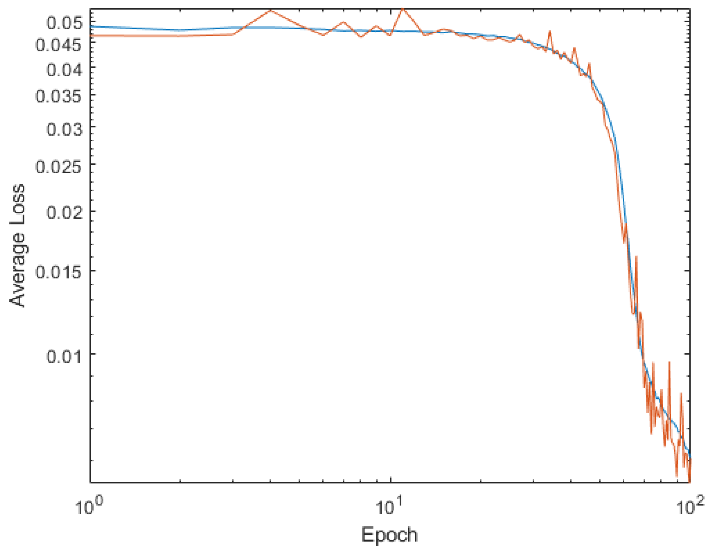
Applying the modifications, instead, the loss reaches 0.0066686 in the learning patterns and 0.006050894 in the validation patterns. Figure 25 shows that similar to the previous case, the loss evolution happens from the 50th epoch on.
The goal function follows the next equation:
z = 1 + c o s ( 12 x 2 + y 2 ) 0.5 ( x 2 + y 2 ) + 2   x ,   y   [ 0.95 ,   1 ]
where z is the desired output and x and y are the inputs to the network. After analyzing the patterns, in the case of the standard SGD learning, all the worst learned patterns have a high negative cos(φ) value with respect to the average, and the modules relationship is over 100 in all the cases; this can be seen in Figure 26. This means that the worst learned patterns are pushing all the training in the opposite direction to the rest of the patterns learning.
In comparison, the best learned patterns are partially aligned to the average value and their modules’ relationships to the average are as high as the worst learned ones, as can be seen in Figure 27. This means that the patterns are poorly learned in general and the network is not able to offer a satisfactory output to the given inputs for this particular case.
On the contrary, using the modified version with dynamic alpha and drop-out, the results are much better. The worst learned patterns are all highly aligned with the average, having also their modules’ relationships smaller than before, as Figure 28 shows. In the case of the better learned patterns, the situation is slightly better than before, as the modules’ relationships to the average are lower; this can be seen in Figure 29. With all these data, we can say that the network probably needs to be modified to be able to learn this particular function properly.

4.5. Goldstein Prize Function

This last function has the following equation:
z = 1 2.427 [ l o g ( [ 1 + ( x + y + 1 ) 2 ( 19 14 x + 3 x 2 14 y + 6 x y + 3 y 2 ) ] [ 30     + ( 2 x 3 y ) 2 ( 18 32 x + 12 x 2 + 48 y 36 x y + 27 y 2 ) ] ) 8.693 ]   x ,   y   [ 0.95 ,   1 ]
where z is the wanted output for the network and x and y are its inputs. After training the network, the obtained results with the standard SGD were 0.001452047 in the training patterns and 0.000901638 in the validation ones. Figure 30 shows a continuous descendant in the loss in both training and validation ranges.
On the dynamic alpha and drop-out, the results were 0.001287429 in the training patterns and 0.002754883 in the validation patterns. Figure 31 shows a similar behavior to the normal SGD case, with a noisier state of the validation loss in the final epochs of training.
Analyzing the patterns, the worst learned patterns present a very low value in the cos(φ) and the modules are high in relationship to the average; see Figure 32. In the best learned patterns case, the results are much more aligned and closed in the module relationship to the average; see Figure 33.
In the case of the dynamic alpha and drop-out, the worst learned patterns show a very low cos(φ) and module relationship, making them not relevant for the training; see Figure 34. The best learned patterns instead have much more presence, having much higher values for their cos(φ); see Figure 35.

5. Conclusions

The authors have used different functions regressions problems in order to illustrate the benefits of their proposal. The authors have two main proposals: an adaptive drop-out policy and a dynamic learning ratio policy.
A dynamic learning ratio lets training algorithms converge in fewer epochs than in a conventional training algorithm. The researcher must know that the deeper a weight is in a neural network, the more a training error needs to propagate along more layers in order to calculate the loss gradient according to this particular weight. This propagation makes the error vanish. This effect implies more epochs of training to cause enough change in a deep weight due to this effect. The dynamical learning policy tries to mitigate it. The policy tries to increase the learning ratio when the weight is deeper. The authors think that the neural network does not learn the optimal values until the deepest weights arrive to their optimal values, because the neural network’s output depends on inputs.
On the other hand, a dynamical drop-out allows the system to have a general learning on the first epochs of the training and a more specific learning to those weights that have already being trained and need to gain accuracy. This is obtained by making the dropping probability bigger in the first stages of leaning and making it smaller through the process, being sufficiently low at the final stages when the loss is low and the resulting gradient is also. With low drop-out, the remaining information of this gradient is not lost, and the synaptic weights correct the final touches of accuracy.
Mixing both techniques together allows the system to benefit from the strengths of both of them and compensates one’s flaws with the other. The results can be seen not only in the simplest function but also in the other benchmark functions: that there is indeed a better performance of both techniques applied to the SGD than with the raw standard SGD.

6. Future Works

As future works, from here, we could follow different paths:
  • To analyze the SWARM intelligence as an algorithm, using the example of a shallow network.
  • To try to apply recursiveness in the shallow neural network alongside the obtained SGD modifications to try to see if the performance is improved.
  • To use pruning algorithms as a basis in order to identify the weakest parts of the network and then reinforce them.

Author Contributions

Conceptualization A.T.-F.-B. and E.Z.; methodology, E.Z.; software, A.T.-F.-B.; validation, E.Z. and U.F.-G.; formal analysis, E.Z. and A.T.-F.-B.; investigation, M.C.-O.; resources, U.F.-G.; writing—original draft preparation, C.B.-M.-I. and E.Z.; writing—review and editing, U.F.-G., C.B.-M.-I. and A.T.-F.-B. All authors have read and agreed to the published version of the manuscript.

Funding

The current study has been sponsored by the Government of the Basque Country-ELKARTEK21/10 KK-2021/00014 (“Estudio de nuevas técnicas de inteligencia artificial basadas en Deep Learning dirigidas a la optimización de procesos industriales”) research program.

Data Availability Statement

The different codes and diagrams are available online at https://github.com/AdrianTeso/BasqueNetPublic.

Conflicts of Interest

The authors declare no conflict of interest.

References

  1. Robbins, H.; Monro, S. A Stochastic Approximation Method. Ann. Math. Stat. 1951, 22, 400–407. [Google Scholar] [CrossRef]
  2. Jha, R.; Jha, N.N.; Lele, M.M. Stochastic gradient descent algorithm for the predictive modelling of grate combustion and boiler dynamics. ISA Trans. 2022. [Google Scholar] [CrossRef]
  3. Bernstein, J.; Wang, Y.-X.; Azizzadenesheli, K.; Anandkumar, A. signSGD: Compressed Optimisation for Non-Convex Problems. arXiv 2018, arXiv:1802.04434. [Google Scholar]
  4. Xu, X.; Kamilov, U.S. SignProx: One-bit Proximal Algorithm for Nonconvex Stochastic Optimization. In Proceedings of the ICASSP 2019—2019 IEEE International Conference on Acoustics, Speech and Signal Processing (ICASSP), Brighton, UK, 12–17 May 2019; pp. 7800–7804. [Google Scholar] [CrossRef] [Green Version]
  5. Sun, T.; Li, D. Sign Stochastic Gradient Descents without bounded gradient assumption for the finite sum minimization. Neural Netw. 2022, 149, 195–203. [Google Scholar] [CrossRef] [PubMed]
  6. Sun, T.; Tang, K.; Li, D. Gradient Descent Learning With Floats. IEEE Trans. Cybern. 2020, 52, 1763–1771. [Google Scholar] [CrossRef]
  7. Geron, A. Hands-On Machine Learning with Scikit-Learn, Keras, and TensorFlow: Concepts, Tools, and Techniques to Build Intelligent Systems, 2nd ed.; O’Reilly Media, Inc.: Sebastopol, CA, USA, 2019. [Google Scholar]
  8. Torres, J. Python Deep Learning, 1.0; MARCOMBO, S.L.: Barcelona, Spain, 2020. [Google Scholar]
  9. Kim, P. MATLAB Deep Learning; Springer: Berlin/Heidelberg, Germany, 2017. [Google Scholar]
  10. Wani, M.A.; Afzal, S. A New Framework for Fine Tuning of Deep Networks. In Proceedings of the 2017 16th IEEE International Conference on Machine Learning and Applications (ICMLA), Cancun, Mexico, 18–21 December 2017; pp. 359–363. [Google Scholar] [CrossRef]
  11. Hinton, G.E.; Srivastava, N.; Krizhevsky, A.; Sutskever, I.; Salakhutdinov, R.R. Improving neural networks by preventing co-adaptation of feature detectors. arXiv 2012, arXiv:1207.0580. [Google Scholar]
  12. Srivastava, N.; Hinton, G.; Krizhevsky, A.; Sutskever, I.; Salakhutdinov, R. Dropout: A Simple Way to Prevent Neural Networks from Overfitting. J. Mach. Learn. Res. 2014, 15, 1929–1958. [Google Scholar]
  13. Duchi, J.; Hazan, E.; Singer, Y. Adaptive Subgradient Methods for Online Learning and Stochastic Optimization. J. Mach. Learn. Res. 2011, 12, 2121–2159. [Google Scholar]
  14. Giannakas, F.; Troussas, C.; Voyiatzis, I.; Sgouropoulou, C. A deep learning classification framework for early prediction of team-based academic performance. Appl. Soft Comput. 2021, 106, 107355. [Google Scholar] [CrossRef]
  15. Fang, J.-K.; Fong, C.-M.; Yang, P.; Hung, C.-K.; Lu, W.-L.; Chang, C.-W. AdaGrad Gradient Descent Method for AI Image Management. In Proceedings of the 2020 IEEE International Conference on Consumer Electronics—Taiwan (ICCE-Taiwan), Taoyuan, Taiwan, 28–30 September 2020; pp. 1–2. [Google Scholar] [CrossRef]
  16. Wei, H.; Zhang, X.; Fang, Z. An Adaptive Quasi-Hyperbolic Momentum Method Based on AdaGrad+ Strategy. In Proceedings of the 2022 International Conference on Image Processing, Computer Vision and Machine Learning (ICICML), Xi’an, China, 28–30 October 2022; pp. 649–654. [Google Scholar] [CrossRef]
  17. Li, H.; Li, X.; Dong, H.; Han, F.; Wang, C. Full-waveform inversion with adversarial losses via deep learning. J. Appl. Geophys. 2022, 205, 104763. [Google Scholar] [CrossRef]
  18. Chakrabarti, K.; Chopra, N. Generalized AdaGrad (G-AdaGrad) and Adam: A State-Space Perspective. In Proceedings of the 2021 60th IEEE Conference on Decision and Control (CDC), Austin, TX, USA, 13–15 December 2021; pp. 1496–1501. [Google Scholar] [CrossRef]
  19. Traoré, C.; Pauwels, E. Sequential convergence of AdaGrad algorithm for smooth convex optimization. Oper. Res. Lett. 2021, 49, 452–458. [Google Scholar] [CrossRef]
  20. Reddy, R.V.K.; Rao, B.S.; Raju, K.P. Handwritten Hindi Digits Recognition Using Convolutional Neural Network with RMSprop Optimization. In Proceedings of the 2018 Second International Conference on Intelligent Computing and Control Systems (ICICCS), Madurai, India, 14–15 June 2018; pp. 45–51. [Google Scholar] [CrossRef]
  21. Khaniki, M.A.L.; Hadi, M.B.; Manthouri, M. Feedback Error Learning Controller based on RMSprop and Salp Swarm Algorithm for Automatic Voltage Regulator System. In Proceedings of the 2020 10th International Conference on Computer and Knowledge Engineering (ICCKE), Mashhad, Iran, 29–30 October 2020; pp. 425–430. [Google Scholar] [CrossRef]
  22. Xu, D.; Zhang, S.; Zhang, H.; Mandic, D.P. Convergence of the RMSProp deep learning method with penalty for nonconvex optimization. Neural Netw. 2021, 139, 17–23. [Google Scholar] [CrossRef]
  23. Yu, Y.; Zhang, L.; Chen, L.; Qin, Z. Adversarial Samples Generation Based on RMSProp. In Proceedings of the 2021 IEEE 6th International Conference on Signal and Image Processing (ICSIP), Nanjing, China, 9–11 October 2021; pp. 1134–1138. [Google Scholar] [CrossRef]
  24. Zou, F.; Shen, L.; Jie, Z.; Zhang, W.; Liu, W. A Sufficient Condition for Convergences of Adam and RMSProp. In Proceedings of the 2019 IEEE/CVF Conference on Computer Vision and Pattern Recognition (CVPR), Long Beach, CA, USA, 16–20 June 2019; pp. 11119–11127. [Google Scholar] [CrossRef] [Green Version]
  25. Zaheer, R.; Shaziya, H. A Study of the Optimization Algorithms in Deep Learning. In Proceedings of the 2019 Third International Conference on Inventive Systems and Control (ICISC), Coimbatore, India, 10–11 January 2019; pp. 536–539. [Google Scholar] [CrossRef]
  26. Liu, D.; He, W.; Zhang, C. The research and optimization on levenberg-marquard algorithm in neural net. In Proceedings of the 2017 IEEE 2nd Advanced Information Technology, Electronic and Automation Control Conference (IAEAC), Chongqing, China, 25–26 March 2017; pp. 2442–2446. [Google Scholar] [CrossRef]
  27. Xiangmei, L.; Zhi, Q. The application of Hybrid Neural Network Algorithms in Intrusion Detection System. In Proceedings of the 2011 International Conference on E-Business and E-Government (ICEE), Shanghai, China, 6–8 May 2011; pp. 1–4. [Google Scholar] [CrossRef]
  28. KUcak; Oke, G. RBF neural network controller based on OLSSVR. In Proceedings of the 2013 9th Asian Control Conference (ASCC), Istanbul, Turkey, 23–26 June 2013; pp. 1–6. [Google Scholar] [CrossRef]
  29. Yadav, A.K.; Singh, A.; Malik, H.; Azeem, A. Cost Analysis of Transformer’s Main Material Weight with Artificial Neural Network (ANN). In Proceedings of the 2011 International Conference on Communication Systems and Network Technologies, Katra, Jammu, India, 3–5 June 2011; pp. 184–187. [Google Scholar] [CrossRef]
  30. Yadav, A.K.; Azeem, A.; Singh, A.; Malik, H.; Rahi, O. Application Research Based on Artificial Neural Network (ANN) to Predict No-Load Loss for Transformer’s Design. In Proceedings of the 2011 International Conference on Communication Systems and Network Technologies, Katra, Jammu, India, 3–5 June 2011; pp. 180–183. [Google Scholar] [CrossRef]
  31. Ucak, K.; Oke, G. Adaptive fuzzy PID controller based on online LSSVR. In Proceedings of the 2012 International Symposium on Innovations in Intelligent Systems and Applications, Trabzon, Turkey, 2–4 July 2012; pp. 1–7. [Google Scholar] [CrossRef]
  32. Levenberg, K. A method for the solution of certain non-linear problems in least squares. Q. Appl. Math. 1944, 2, 164–168. [Google Scholar] [CrossRef] [Green Version]
  33. Almalki, M.M.; Alaidarous, E.S.; Maturi, D.A.; Raja, M.A.Z.; Shoaib, M. A Levenberg–Marquardt Backpropagation Neural Network for the Numerical Treatment of Squeezing Flow With Heat Transfer Model. IEEE Access 2020, 8, 227340–227348. [Google Scholar] [CrossRef]
  34. Teso-Fz-Betoño, A.; Zulueta, E.; Cabezas-Olivenza, M.; Teso-Fz-Betoño, D.; Fernandez-Gamiz, U. A Study of Learning Issues in Feedforward Neural Networks. Mathematics 2022, 10, 3206. [Google Scholar] [CrossRef]
  35. Roux, N.L.; Schmidt, M.; Bach, F. A Stochastic Gradient Method with an Exponential Convergence Rate for Finite Training Sets. arXiv 2012, arXiv:1202.6258. [Google Scholar]
  36. Defazio, A.; Bach, F.; Lacoste-Julien, S. SAGA: A Fast Incremental Gradient Method With Support for Non-Strongly Convex Composite Objectives. arXiv 2014, arXiv:1407.0202. [Google Scholar]
  37. Jain, P.; Kakade, S.M.; Kidambi, R.; Netrapalli, P.; Sidford, Y.A. Accelerating Stochastic Gradient Descent. arXiv 2017, arXiv:1704.08227. [Google Scholar]
  38. Yang, Z. Adaptive stochastic conjugate gradient for machine learning. Expert Syst. Appl. 2022, 206, 117719. [Google Scholar] [CrossRef]
  39. Wang, P.; Zheng, N. Convergence analysis of asynchronous stochastic recursive gradient algorithms. Knowl.-Based Syst. 2022, 252, 109312. [Google Scholar] [CrossRef]
  40. Li, Z.; Shang, T.; Liu, X.; Qian, P.; Zhang, Y. Advanced multi-feedback stochastic parallel gradient descent wavefront correction in free-space optical communication. Opt. Commun. 2023, 533, 129268. [Google Scholar] [CrossRef]
  41. Hu, Q.; Zhen, L.; Mao, Y.; Zhu, S.; Zhou, X.; Zhou, G. Adaptive stochastic parallel gradient descent approach for efficient fiber coupling. Opt. Express 2020, 28, 13141–13154. [Google Scholar] [CrossRef] [PubMed]
  42. Phong, L.T.; Phuong, T.T. Differentially private stochastic gradient descent via compression and memorization. J. Syst. Arch. 2023, 135, 102819. [Google Scholar] [CrossRef]
  43. Roberts, L.; Smyth, E. A simplified convergence theory for Byzantine resilient stochastic gradient descent. EURO J. Comput. Optim. 2022, 10, 100038. [Google Scholar] [CrossRef]
  44. Blanchard, P.; Mhamdi, E.M.E.; Guerraoui, R.; Stainer, J. Machine Learning with Adversaries: Byzantine Tolerant Gradient Descent. Adv. Neural Inf. Process. Syst. 2017, 30. [Google Scholar]
  45. Chen, G.; Qu, C.K.; Gong, P. Anomalous diffusion dynamics of learning in deep neural networks. Neural Netw. 2022, 149, 18–28. [Google Scholar] [CrossRef] [PubMed]
  46. Fjellström, C.; Nyström, K. Deep learning, stochastic gradient descent and diffusion maps. J. Comput. Math. Data Sci. 2022, 4, 100054. [Google Scholar] [CrossRef]
  47. Ojha, V.; Nicosia, G. Backpropagation Neural Tree. Neural Netw. 2022, 149, 66–83. [Google Scholar] [CrossRef] [PubMed]
  48. Senthil, R.; Narayanan, B.; Velmurugan, K. Develop the hybrid Adadelta Stochastic Gradient Classifier with optimized feature selection algorithm to predict the heart disease at earlier stage. Meas. Sens. 2023, 25, 100602. [Google Scholar] [CrossRef]
  49. Ba, J.; Frey, B. Adaptive dropout for training deep neural networks. Adv. Neural Inf. Process. Syst. 2013, 26. [Google Scholar]
  50. Li, H.; Weng, J.; Mao, Y.; Wang, Y.; Zhan, Y.; Cai, Q.; Gu, W. Adaptive Dropout Method Based on Biological Principles. IEEE Trans. Neural Netw. Learn. Syst. 2021, 32, 4267–4276. [Google Scholar] [CrossRef] [PubMed]
  51. Mirzadeh, S.I.; Farajtabar, M.; Ghasemzadeh, H. Dropout as an Implicit Gating Mechanism For Continual Learning. In Proceedings of the 2020 IEEE/CVF Conference on Computer Vision and Pattern Recognition Workshops (CVPRW), Seattle, WA, USA, 14–19 June 2020; pp. 945–951. [Google Scholar] [CrossRef]
  52. Chen, Y.; Yi, Z. Adaptive sparse dropout: Learning the certainty and uncertainty in deep neural networks. Neurocomputing 2021, 450, 354–361. [Google Scholar] [CrossRef]
  53. LeJeune, D.; Javadi, H.; Baraniuk, R.G. The Flip Side of the Reweighted Coin: Duality of Adaptive Dropout and Regularization. arXiv 2021, arXiv:2106.07769. [Google Scholar]
  54. Surjanovic, S.; Bingham, D. Virtual Library of Simulation Experiments: Test functions and Datasets. 2013. Available online: https://www.sfu.ca/~ssurjano/index.html (accessed on 6 August 2022).
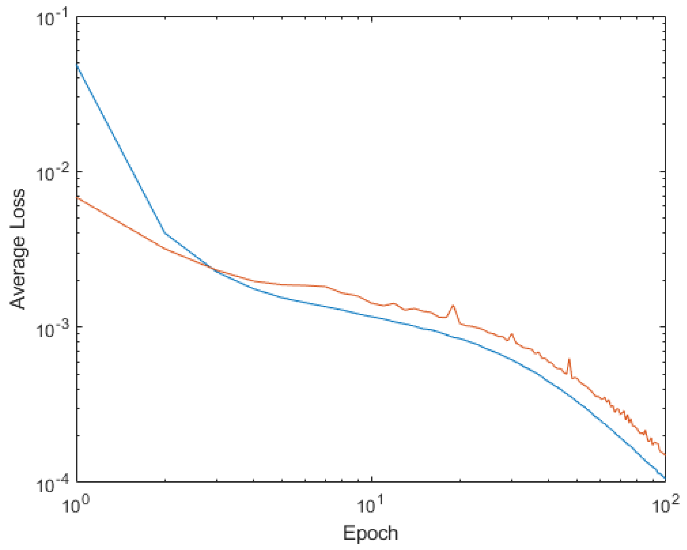
Figure 1. Average loss on training patterns in blue and validation patterns in orange for the standard SGD learning of Mexican Hat.
Mathematics 11 01183 g001
Figure 2. Average loss on training patterns in blue and validation patterns in orange for Dynamic alpha SGD of Mexican Hat.
Mathematics 11 01183 g002
Figure 3. Unified worst learned patterns cos(φ) on the (left) and | L o s s W n | relationship to the average | L o s s W n | on the (right) for dynamic alpha modification for Dynamic alpha SGD of Mexican Hat.
Mathematics 11 01183 g003
Figure 4. Unified best learned patterns cos(φ) on the (left) and | L o s s W n | relationship to the average | L o s s W n | on the (right) for dynamic alpha modification for Dynamic alpha of Mexican Hat.
Mathematics 11 01183 g004
Figure 5. Average loss on training patterns in blue and validation patterns in orange for the Dynamic drop-out SGD of Mexican Hat.
Mathematics 11 01183 g005
Figure 6. Unified worst learned patterns cos(φ) on the (left) and | L o s s W n | relationship to the average | L o s s W n | on the (right) for the dynamic drop-out modification for the Dynamic drop-out SGD of Mexican Hat.
Mathematics 11 01183 g006
Figure 7. Unified best learned patterns cos(φ) on the (left) and | L o s s W n | relationship to the average | L o s s W n | on the (right) for dynamic drop-out for the Dynamic drop-out SGD of Mexican Hat.
Mathematics 11 01183 g007
Figure 8. Average loss on training patterns in blue and validation patterns in orange for the Dynamic drop-out and Dynamic alpha SGD of Mexican Hat.
Mathematics 11 01183 g008
Figure 9. Resulting error on the validation patterns. The dynamic alpha modification on the (left) and the mixed dynamic alpha and drop-out on the (right).
Mathematics 11 01183 g009
Figure 10. Unified worst learned patterns cos(φ) on the (left) and | L o s s W n | relationship to the average | L o s s W n | on the (right) for the dynamic alpha and drop-out modifications used together.
Mathematics 11 01183 g010
Figure 11. Unified best learned patterns cos(φ) on the (left) and | L o s s W n | relationship to the average | L o s s W n | on the (right) for the dynamic alpha and drop-out modifications used together.
Mathematics 11 01183 g011
Figure 12. Average loss on training patterns in blue and validation patterns in orange for Standard SGD of Ackley function.
Mathematics 11 01183 g012
Figure 13. Unified worst learned patterns cos(φ) on the (left) and | L o s s W n | relationship to the average | L o s s W n | on the (right) for the Ackley function using the standard SGD algorithm.
Mathematics 11 01183 g013
Figure 14. Unified best learned patterns cos(φ) on the (left) and | L o s s W n | relationship to the average | L o s s W n | on the (right) for the Ackley function using the standard SGD algorithm.
Mathematics 11 01183 g014
Figure 15. Average loss on training patterns in blue and validation patterns in orange for Dynamic alpha and Dynamic drop-out mixed together SGD of Ackley function.
Mathematics 11 01183 g015
Figure 16. Unified worst learned patterns cos(φ) on the (left) and | L o s s W n | relationship to the average | L o s s W n | on the (right) for the Ackley function using the dynamic alpha and drop-out modifications for Dynamic alpha and Dynamic drop-out mixed together SGD of Ackley function.
Mathematics 11 01183 g016
Figure 17. Unified best learned patterns cos(φ) on the (left) and | L o s s W n | relationship to the average | L o s s W n | on the (right) for the Ackley function using the dynamic alpha and drop-out modifications for Dynamic alpha and Dynamic drop-out mixed together SGD of Ackley function.
Mathematics 11 01183 g017
Figure 18. Average loss on training patterns in blue and validation patterns in orange for Standard SGD of Cross-in-Tray function.
Mathematics 11 01183 g018
Figure 19. Average loss on training patterns in blue and validation patterns in orange for Dynamic alpha and Dynamic drop-out mixed together SGD of Cross-in-Tray.
Mathematics 11 01183 g019
Figure 20. Unified worst learned patterns cos(φ) on the (left) and | L o s s W n | relationship to the average | L o s s W n | on the (right) for the Cross-in-Tray function using the standard SGD.
Mathematics 11 01183 g020
Figure 21. Unified best learned patterns cos(φ) on the (left) and | L o s s W n | relationship to the average | L o s s W n | on the (right) for the Cross-in-Tray function using the standard SGD.
Mathematics 11 01183 g021
Figure 22. Unified worst learned patterns cos(φ) on the (left) and | L o s s W n | relationship to the average | L o s s W n | on the (right) for the Cross-in-Tray function using the dynamic alpha and drop-out.
Mathematics 11 01183 g022
Figure 23. Unified best learned patterns cos(φ) on the (left) and | L o s s W n | relationship to the average | L o s s W n | on the (right) for the Cross-in-Tray function using the dynamic alpha and drop-out.
Mathematics 11 01183 g023
Figure 24. Average loss on training patterns in blue and validation patterns in orange for Standard SGD of Drop-Wave function.
Mathematics 11 01183 g024
Figure 25. Average loss on training patterns in blue and validation patterns in orange for Dynamic alpha and Dynamic drop-out mixed together SGD of Drop-Wave function.
Mathematics 11 01183 g025
Figure 26. Unified worst learned patterns cos(φ) on the (left) and | L o s s W n | relationship to the average | L o s s W n | on the (right) for the drop-wave function using the standard SGD algorithm.
Mathematics 11 01183 g026
Figure 27. Unified best learned patterns cos(φ) on the (left) and | L o s s W n | relationship to the average | L o s s W n | on the (right) for the drop-wave function using the standard SGD algorithm.
Mathematics 11 01183 g027
Figure 28. Unified worst learned patterns cos(φ) on the (left) and | L o s s W n | relationship to the average | L o s s W n | on the (right) for the drop-wave function using the modified SGD with dynamic alpha and drop-out.
Mathematics 11 01183 g028
Figure 29. Unified best learned patterns cos(φ) on the (left) and | L o s s W n | relationship to the average | L o s s W n | on the (right) for the drop-wave function using the modified SGD with dynamic alpha and drop-out.
Mathematics 11 01183 g029
Figure 30. Average loss on training patterns in blue and validation patterns in orange for Standard SGD of Goldstein Prize function.
Mathematics 11 01183 g030
Figure 31. Average loss on training patterns in blue and validation patterns in orange for Dynamic alpha and Dynamic Drop-out mixed together SGD of Goldstein Prize function.
Mathematics 11 01183 g031
Figure 32. Unified worst learned patterns cos(φ) on the (left) and | L o s s W n | relationship to the average | L o s s W n | on the (right) for the Goldstein Prize function using the standard SGD algorithm.
Mathematics 11 01183 g032
Figure 33. Unified best learned patterns cos(φ) on the (left) and | L o s s W n | relationship to the average | L o s s W n | on the (right) for the Goldstein Prize function using the standard SGD algorithm.
Mathematics 11 01183 g033
Figure 34. Unified worst learned patterns cos(φ) on the (left) and | L o s s W n | relationship to the average | L o s s W n | on the (right) for the Goldstein Prize function using the dynamic alpha and drop-out.
Mathematics 11 01183 g034
Figure 35. Unified best learned patterns cos(φ) on the (left) and | L o s s W n | relationship to the average | L o s s W n | on the (right) for the Goldstein Prize function using the dynamic alpha and drop-out.
Mathematics 11 01183 g035
Disclaimer/Publisher’s Note: The statements, opinions and data contained in all publications are solely those of the individual author(s) and contributor(s) and not of MDPI and/or the editor(s). MDPI and/or the editor(s) disclaim responsibility for any injury to people or property resulting from any ideas, methods, instructions or products referred to in the content.