Local Property of Depth Information in 3D Images and Its Application in Feature Matching

Abstract

In image registration or image matching, the feature extracted by using the traditional methods does not include the depth information which may lead to a mismatch of keypoints. In this paper, we prove that when the camera moves, the ratio of the depth difference of a keypoint and its neighbor pixel before and after the camera movement approximates a constant. That means the depth difference of a keypoint and its neighbor pixel after normalization is invariant to the camera movement. Based on this property, all the depth differences of a keypoint and its neighbor pixels constitute a local depth-based feature, which can be used as a supplement of the traditional feature. We combine the local depth-based feature with the SIFT feature descriptor to form a new feature descriptor, and the experimental results show the feasibility and effectiveness of the new feature descriptor.

1. Introduction

In the era of global automation and artificial intelligence, image and vision processing technologies play an important role in many areas, such as autonomous driving, 3D reconstruction, and positioning and navigation. Image matching, also known as image registration or correspondence, is a key and fundamental problem in these complex tasks [1]. Image matching refers to establishing a corresponding relationship between the two images (image pair) before and after the camera moves (or the camera does not move, the object moves), in which two pixels from the two images corresponding to the same object point consist of a pair. Image matching roughly includes three steps: image key feature extraction and positioning, feature description, and feature matching. The key features of the image, also called keypoints, refer to points with particularly prominent properties in a certain aspect, such as corner points and points that are invariant to affine transformation. Feature matching refers to identifying and matching pixels with the same or similar features in two images [2].

Regarding the extraction of image keypoints, Lowe proposed a method to extract unique invariant features from images (SIFT, scale-invariant feature transform) [3]. These features are invariant to the scale and rotation of the image and are shown to provide robust matching of affine distortions, changes in 3D viewpoint, the addition of noise, and changes in illumination. Subsequently, Bay et al. proposed a new scale and rotation invariant interest point detector and descriptor SURF (speeded up robust features) [4], which improved efficiency while maintaining repeatability, specificity, and robustness. Alahi et al. proposed a new keypoint descriptor [5], which was inspired by the human visual system, and more precisely, from the retina, called fast retinal keypoints (FREAK). In terms of key feature matching, Bellavia designed a general matching framework with a new matching strategy and a new local spatial filter [6], combining multiple strategies, including pre-screening as well as many-to-many and symmetric matching, to find and adjust keypoint neighborhood consistency, enabling global improvements to each individual strategy. Another approach for robust feature matching between two images captured from different viewpoints is view synthesis [7,8,9,10]. This method generates multiple affine or projective deformations of each of the two images, then extracts and matches the features of each deformation. Toft proposed that CNN-based depth inferred from a single RGB image is very helpful, which can be used to pre-distort images and correct perspective distortion, significantly enhancing SIFT and BRISK capabilities [11]. However, the method is mainly for situations where the camera is looking at the same scene but in the opposite direction.

Most of the current image matching methods work on two images with small changes. When the image pair parallax is large, there is a possibility that similar objects both far and nearby are considered to be the same object. The reason is that the existing matching methods do not consider the depth information of the image, that is, the distance of the object from the camera. Recently, Chen et al. proposed a new de-mismatching algorithm that combines depth prediction and feature matching [12], but they simply used the key depth information as an indicator for threshold judgment and did not use image depth information as a part of the feature.

In 3D computer graphics and computer vision, the depth map records the distance from the shooting device to each point in the scene, where each pixel value of the depth map represents the distance from the object plane to the camera center [13]. Since the depth map contains the depth information of the scene, it can be combined with the traditional RGB image to form the RGBD image which extends the image information from two-dimensional to three-dimensional and can be calculated and used for 3D shape simulation and 3D reconstruction. There are many methods to obtain image depth information; 3D cameras (depth cameras) [14,15,16], for examples, LiDAR or Kinect, can be used to obtain depth maps. Binocular stereo vision [17,18] uses the principle of parallax to obtain two images of the measured object from different positions and calculates the positional deviation between the corresponding points of the images to obtain the depth information of the object. Monocular depth estimation [19,20,21,22] trains a neural network to predict the depth map of a single RGB image. There are also many commonly used public RGBD datasets, for examples, SUN RGBD, TUM, SCAN NET, and NYU depth dataset V2. Among them, the NYU dataset consists of video sequences of various indoor scenes recorded by Microsoft Kinect’s RGB and depth cameras [23]. It consists of pairs of RGB and depth frames that are synchronized and densely labeled for each image.

In this paper, we study the property of the depth map and construct a new feature descriptor with depth information on the basis of SIFT. We prove that, when the camera moves, the ratio of the depth difference of a keypoint and its neighbor pixel before and after the camera movement approximates a constant. That means the depth difference of a keypoint and its neighbor pixel after normalization is invariant to the camera movement. Based on this property, all the depth differences of a keypoint and its neighbor pixels constitute a local depth-based feature, which can be used as a supplement of the traditional feature. We combine the local depth-based feature with the SIFT feature descriptor to form a new feature descriptor. To validate the effectiveness of the new feature descriptor, 20 images in the NYU dataset are extracted to form 10 pairs for comparative experiments. The experimental results show that the proposed method can eliminate the wrong matching pairs and improve the accuracy.

In summary, the contributions of this work are as follows:

• We explore the local property of the depth information of image pairs taken before and after the camera movements.
• We prove the local property of the depth information: the ratio of the depth difference of a keypoint and its neighbor pixels before and after the camera movement approximates to a constant.
• Based on the local property, a local depth-based feature descriptor is proposed, which can be used as a supplement of the traditional feature.

The rest of this paper is structured as follows: Related work is discussed in the second section. The third and fourth sections introduce the key features of SIFT and its mismatching problem. Then, the local property of depth information is proved and used for constructing a supplement of the SIFT descriptor. Finally, the experiment results and analysis are given.

2. Related Work

This section gives a brief introduction of existing methods on image matching and depth information.

2.1. Image Matching

In 2004, Lowe et al. proposed the famous scale-invariant feature transform (SIFT) algorithm, with the features extracted being invariant to the scale and rotation of the image. The details of the SIFT algorithm will be given in the next section. However, SIFT has some limits. For example, it has a mismatch problem produced by the movements of cameras or lack of colors, low search efficiency, etc.

To improve the SIFT algorithm, Abdel constructed a colored SIFT (CSIFT) descriptor in color invariant space [24], extending the SIFT descriptor to the color space. Bay et al. proposed a new scale and rotation invariant interest point detector and descriptor SURF (speeded up robust features) [4], which used a blob detector based on a Hessian matrix to find the interest points and improved efficiency while maintaining repeatability, specificity, and robustness. However, it relied too much on the gradient direction of the local area pixel in the stage of finding the host direction, which enlarged the error in the subsequent feature matching even if the deviation angle was not large. Rublee et al. proposed directional FAST and Rotating BRIEF algorithms ORB [25], which combined FAST [26] and BRIEF [27] algorithms to form new feature detectors and feature descriptors. The ORB method used a fast and accurate corner orientation component with intensity centroid and the efficient computation of BRIEF characteristics which enabled real-time computation. However, it is not scale-invariant and is sensitive to brightness. Balammal et al. proposed an image local feature extraction method based on SIFT and KAZE fusion [28], which preserves the unique property of an image representation. In this method, the bag of visual word model [29] was introduced to enhance the scalability and the relevance feedback system was included to reduce the semantic gap. Tang et al. proposed an improved SIFT algorithm [30] in which a stability factor was added in scale space for accurate matching, and the feature descriptor was simplified to shorten the matching time. Feng et al. proposed the concept of inter-feature relative azimuth and distance (IFRAD) [31] and constructed the corresponding feature descriptor to improve the scale invariance and matching accuracy. In this method, the FAST method [26] is used to detect a series of features, and the criteria based on IFRAD is used to select the stable features. Finally a special feature-similarity evaluator was designed to match features in two images. Chung et al. proposed a new cooperative RANSAC (COOSAC) [32] method using a geometry histogram-based (GH-based) constructed to reduce the correspondence set for remote sensing matching [33].

Besides the SIFT descriptor and its variants, some other descriptors, especially for 3D images, were proposed. Tombari proposed a local 3D descriptor for surface matching [34], which was located at the intersection between signatures and histograms so that a better balance between descriptive and robust was possible. Later, they proposed the SHOT method aimed at a more favorable balance between descriptive power and robustness [35]. Based on the SHOT descriptor, Prakhya et al. proposed the B-SHOT descriptor, a binary 3D feature descriptor for keypoint matching on 3D point clouds [36]. In this method, a binary quantization method converting a real valued vector to a binary vector is proposed which reduces the memory requirements in keypoint matching. Steder et al. proposed the normal-aligned radial features (NARF) for feature descriptor calculation in 3D range data [37], which considered object boundary information and the surface structure and extracted the keypoints located on the stable areas for normal estimation or descriptor calculation.

2.2. Depth Information Estimation

Deep neural network is the state-of-the-art technology for obtaining depth information or a depth map. The current mainstream method of depth information estimation is monocular depth estimation [38,39,40], which alleviates the limitation of binocular estimation due to its high cost, large size, and fixed location.

In 2017, Ummenhofer et al. proposed DeMoN, which is the first depth network that learns to estimate depth and camera motion from two unconstrained images [20]. Unlike networks that estimate depth from a single image, DeMoN can take advantage of motion parallax, a powerful clue that can be generalized to new types of scenes. However, it does not have the flexibility of the classic approach when it comes to dealing with cameras with different intrinsic parameters. So, their next challenge was to lift this restriction and extend this work to more than two images. In 2019, they proposed a new convolution CAM-Convs [21], which could take camera parameters into account, thus allowing neural networks to learn to calibrate perceptual patterns, which greatly improved the generalization ability of depth prediction networks. In 2020, they proposed DeepTAM, a fully learned camera tracking and depth mapping estimation system based on dense keyframes [22]. For tracking, the small attitude increment between the current camera image and the composite viewpoint is estimated.

Reza Mahjourian et al. proposed a method for unsupervised learning of depth and ego-motion from monocular videos [41]. This method explicitly considered the inferred 3D geometry of the whole scene and enforced consistency of the estimated 3D point clouds and ego-motion across consecutive frames. Jun Wang et al. proposed a self-supervised framework for RGB-guided depth enhancement [42]. In this method, the dependency between RGB and depth was exploited and a multi-scale edge-guided network model was designed for the learning of depth information enhancement.

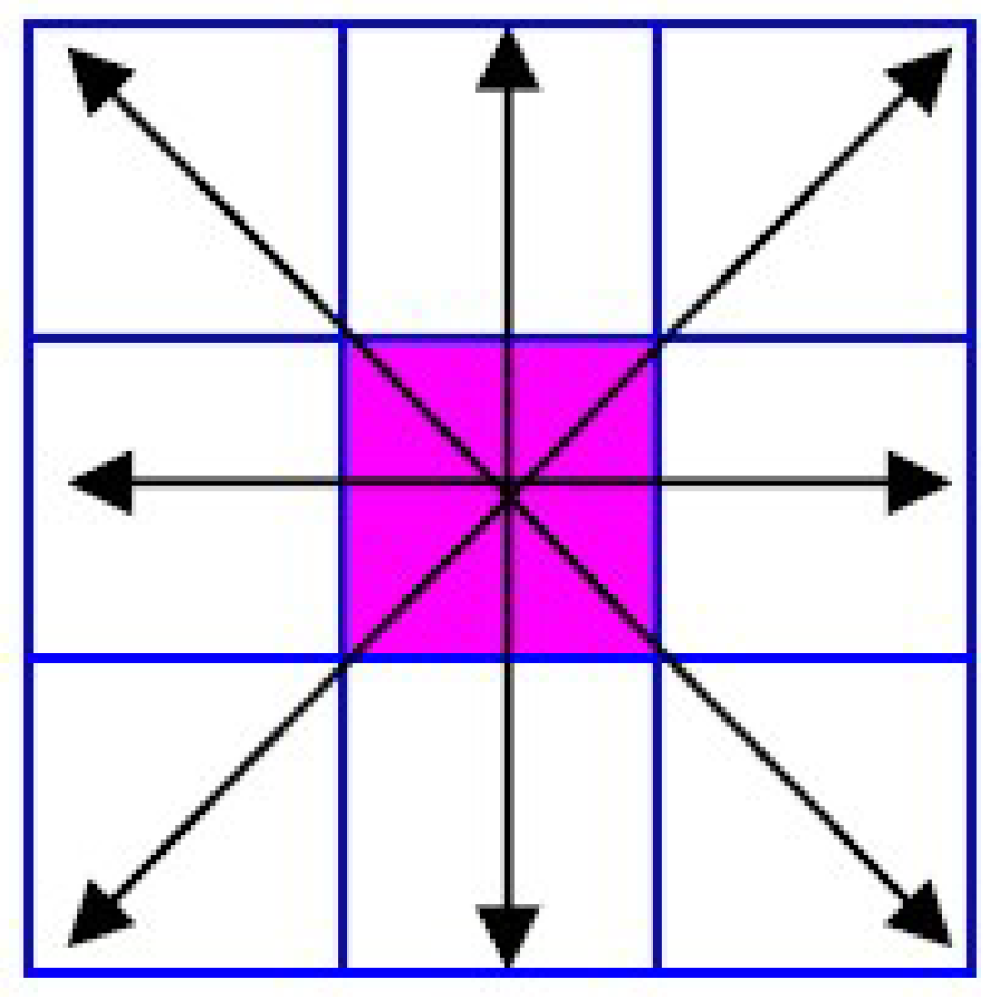
3. The SIFT Key Features

Scale-invariant feature transform (SIFT) [3] is an algorithm used to detect and describe local features of images, effectively solving the problems of object rotation, scaling, translation, image affine/projection transformation, lighting effects, object occlusion, fragmentation scenes, etc. The Gaussian Laplacian of the image reflects the second-order variation of the color or brightness of the image, and its maximum and minimum points can be used as the keypoints of the image [3]. The SIFT algorithm introduces scale variables $\sigma$, approximates the Laplacian operator with the difference of Gaussian (DoG, difference of Gaussian) in the scale space [43], and finds three-dimensional (space + scale) extreme points in the Gaussian difference images as keypoints. Finally, the gradient distribution information of the surrounding neighborhood of each keypoint is expressed as a 128-dimensional vector used as the feature descriptor.

• Scale space and Gaussian difference space

The scale space $L(x,y,\sigma )$ of the image $I(x,y)$ is defined as the convolution of the variable-scale Gaussian function $G(x,y,\sigma )$ with the original image $I(x,y)$ [43]:

$$L(x,y,\sigma )=G(x,y,\sigma )\ast I(x,y)$$

(1)

$$G(x,y,\sigma )=\frac{1}{2\pi {\sigma }^2}{e}^{-\frac{{(x-m/2)}^2+{(y-n/2)}^2}{2{\sigma }^2}}$$

(2)

where $(x,y)$ represents the pixel location of the image, and $m\times n$ are the size of the two-dimensional template of the Gaussian function. In addition, $\sigma$ is the scale space factor, the smaller the $\sigma$ value, the smaller the local area used for image smoothing. The large scale reflects the contour characteristics of the image, while the small scale reflects the detailed characteristics of the image.

The difference of two nearby scale spaces separated by a constant multiplicative factor k is defined as the difference of Gaussian (DoG) space:

$$D(x,y,\sigma )=L(x,y,k\sigma )-L(x,y,\sigma )=\left(G(x,y,k\sigma )-G(x,y,\sigma )\right)\ast I(x,y)$$

(3)

• Gaussian difference pyramid

For the same physical object in the imaging system, the farther from the center of the camera, the smaller and blurrier the object in the image is. The details of the objects close to the camera can be seen clearly, but the contour profile of the farther object may not be seen completely; on the other hand, the contour profile of the object far from the camera can be exhibited, but the details may be blurred. The SIFT method uses the scale space and the pyramid method to describe this phenomenon and reduce the computational cost [44].

Suppose the original image $I_1(x,y)$ is of size $M\times N$. With different scales ${\sigma }_1$, $k{\sigma }_1$, $k^2{\sigma }_1$, $k^3{\sigma }_1$, and $k^4{\sigma }_1$ where k is a constant, a group of Gaussian difference spaces can be obtained:

$$\begin{array}{cc}\hfill D_1(x,y,{\sigma }_1)& =(G(x,y,k{\sigma }_1)-G(x,y,{\sigma }_1))\ast I_1(x,y)\hfill \\ \hfill D_1(x,y,k{\sigma }_1)& =(G(x,y,k^2{\sigma }_1)-G(x,y,k{\sigma }_1))\ast I_1(x,y)\hfill \\ \hfill D_1(x,y,k^2{\sigma }_1)& =(G(x,y,k^3{\sigma }_1)-G(x,y,k^2{\sigma }_1))\ast I_1(x,y)\hfill \\ \hfill D_1(x,y,k^3{\sigma }_1)& =(G(x,y,k^4{\sigma }_1)-G(x,y,k^3{\sigma }_1))\ast I_1(x,y)\hfill \end{array}$$

(4)

Denote

$$P_1(I_1,{\sigma }_1)=\{D_1(x,y,{\sigma }_1),D_1(x,y,k{\sigma }_1),D_1(x,y,k^2{\sigma }_1),D_1(x,y,k^3{\sigma }_1)\}$$

(5)

Downsample the image $I_1(x,y)$ by a factor of two to obtain an image $I_2(x,y)$ with size $\frac{M}{2}\times \frac{N}{2}$. Taking ${\sigma }_2=2{\sigma }_1$ as the initial scale, a new set of Gaussian difference spaces can be obtained by a calculation similar to Formula (4):

$$P_2(I_2,{\sigma }_2)=\{D_2(x,y,{\sigma }_2),D_2(x,y,k{\sigma }_2),D_2(x,y,k^2{\sigma }_2),D_2(x,y,k^3{\sigma }_2)\}$$

(6)

Two-factor continuous downsampling will produce images $I_3(x,y)\mathrm{and}{I}_4(x,y)$. Let ${\sigma }_3=2{\sigma }_2,{\sigma }_4=2{\sigma }_3$, respectively. Then, the other two Gaussian difference groups $P_3(I_3,{\sigma }_3)$ and $P_4(I_4,{\sigma }_4)$ are obtained similarly. The four groups of Gaussian difference spaces $P_1(I_1,{\sigma }_1)$, $P_2(I_2,{\sigma }_2)$, $P_3(I_3,{\sigma }_3)$, and $P_4(I_4,{\sigma }_4)$ consist of a pyramid.

• Keypoint positioning

The SIFT algorithm selects the three-dimensional (coordinates x, y, and the scale $\sigma$) extreme points in the Gaussian difference pyramid as the keypoints. For each point $(x,y,\sigma )$ in the pyramid, it needs to compare its eight neighbors of the same scale $\sigma$ space, and nine neighbors of adjacent scales $k\sigma$ and $\sigma /k$. In a group of Gaussian difference spaces $P_i(I_i,{\sigma }_i),i=1,\dots ,4$, since the first scale space and the last scale space each have only one neighbor in the scale direction, there are no three-dimensional extreme points. Only the middle two scale spaces of a group of Gaussian difference spaces may exist as extreme points. All Gaussian difference spaces that may have extreme points are listed following:

$$\begin{array}{cc}\hfill & D_1(x,y,k{\sigma }_1),D_1(x,y,k^2{\sigma }_1),D_2(x,y,k{\sigma }_2),D_2(x,y,k^2{\sigma }_2),\hfill \\ \hfill & D_3(x,y,k{\sigma }_3),D_3(x,y,k^2{\sigma }_3),D_4(x,y,k{\sigma }_4),D_4(x,y,k^2{\sigma }_4)\hfill \end{array}$$

(7)

Change scales ${\sigma }_i,i=1,2,3,4$ to the initial scale ${\sigma }_1$:

$$\begin{array}{cc}\hfill & D_1(x,y,k{\sigma }_1),D_1(x,y,k^2{\sigma }_1),D_2(x,y,2k{\sigma }_1),D_2(x,y,2k^2{\sigma }_1),\hfill \\ \hfill & D_3(x,y,4k{\sigma }_1),D_3(x,y,4k^2{\sigma }_1),D_4(x,y,8k{\sigma }_1),D_4(x,y,8k^2{\sigma }_1)\hfill \end{array}$$

(8)

In the SIFT algorithm, taking $k=\sqrt{2}$, then the above list is rewritten as:

$$\begin{array}{cc}\hfill & D_1(x,y,\sqrt{2}{\sigma }_1),D_1(x,y,2{\sigma }_1),D_2(x,y,2\sqrt{2}{\sigma }_1),D_2(x,y,4{\sigma }_1),\hfill \\ \hfill & D_3(x,y,4\sqrt{2}{\sigma }_1),D_3(x,y,8{\sigma }_1),D_4(x,y,8\sqrt{2}{\sigma }_1),D_4(x,y,16{\sigma }_1)\hfill \end{array}$$

(9)

Now we can see that the scale factor uniquely determines the scale space where the extreme point is located.

• Keypoint offset correction

The Gaussian difference pyramid is discrete, and the above calculation of the extreme points can only determine the approximate position of keypoints [45], which may not be a pixel point when transformed to the original images. The offset to the precise position can be calculated by the Taylor expansion.

Let $X={(x,y,\sigma )}^T$ be the approximate position of a keypoint and $\Delta X={(\Delta x,\Delta y,\Delta \sigma )}^T$ be the offset. The Taylor expansion of the DoG function (3) in the precise point is:

$$D(X+\Delta X)\approx D\left(X\right)+\frac{\partial D^T}{\partial X}·\Delta X+\frac{1}{2}\Delta X^T\frac{{\partial }^{2}D}{\partial X^2}\Delta X$$

(10)

Since the keypoint is an extreme point, the derivative of this function with respect to $\Delta X$ is zero:

$$\frac{\partial D(X+\Delta X)}{\partial \Delta X}=0$$

(11)

and the offset of the extreme point can be obtained:

$$\Delta X\approx -{\left(\frac{{\partial }^{2}D}{\partial X^2}\right)}^{-1}\frac{\partial D^T}{\partial X}$$

(12)

When the offset of $\Delta X$ in any dimension (i.e., $\Delta x$, $\Delta y$, or $\Delta \sigma$) is greater than 0.5, the keypoint has been offset to its adjacent point, and the position of the current keypoint must be changed.

• Key feature descriptors

The SIFT algorithm uses gradient information of neighboring pixels around keypoints in the same scale space as key features. The gradient direction is discretized into eight directions as described in Figure 1: up, down, left, right, and the diagonals [46]:

For the detected keypoint $(x,y,\sigma )$ in the DoG pyramid, the 16 × 16 neighborhood of $(x,y,\sigma )$ in the scale space image $L(x,y,\sigma )$ is divided into 16 small blocks of 4 × 4. In every small block, the gradient magnitudes with the same direction are weighted accumulated and form an eight-dimensional vector. All the 8-dimensional vectors of 16 small blocks are collaged to a 128-dimensonal vector, which is the SIFT key feature descriptor.

In the actual calculation, in order to obtain better scale invariance and rotation invariance, the SIFT algorithm also performs operations, such as edge response removal and direction normalization. One may find the detailed description in reference [3].

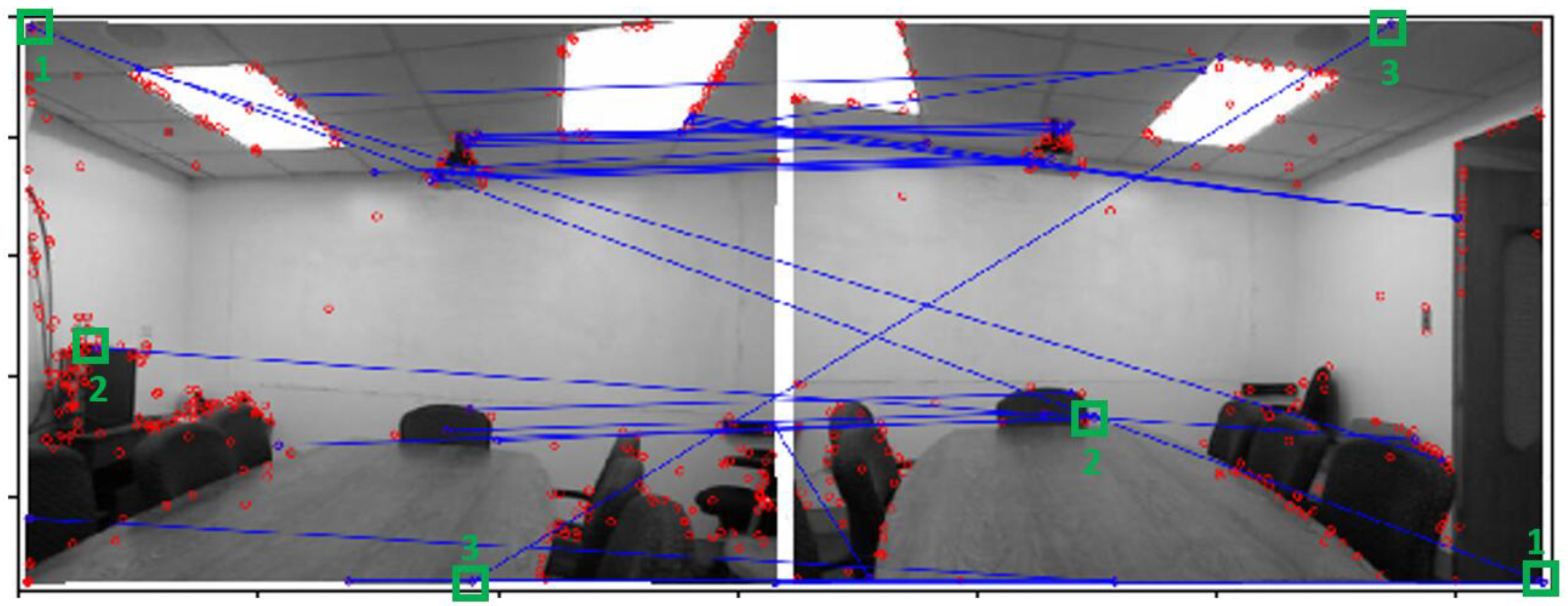
4. False matching Based on SIFT Feature Descriptors

When the parallax of the image pair $(I_1,I_2)$ is not small, the use of basic SIFT feature descriptors may lead to false matching results in subsequent feature matching. For example, Figure 2 shows an image pair taken from different shooting angles in which the SIFT algorithm gives false matching pairs 1, 2, and 3 marked by green boxes. The reason is that the keypoints corresponding to the different object points have similar SIFT features.

In order to alleviate this problem, in this paper, we introduce the depth information of the image, that is, the distance between the object plane and the camera, as the supplement of the SIFT feature. We prove that when the camera moves, the ratio of the depth difference of the keypoint and its neighbor pixels before and after the camera movement approximates a constant. Based on this property, the depth differences of all pixels in the keypoint neighborhood with the keypoint constitute a local depth-based feature used as a supplement of the SIFT feature.

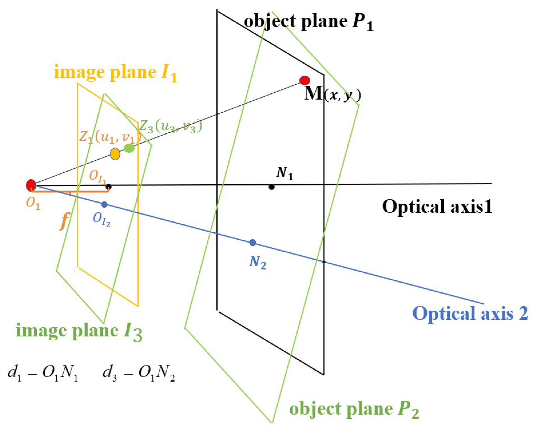
5. Local Property of Depth Information under the Camera Movement

In image registration, an image pair to be matched can be regarded as two image planes generated by the same natural scene before and after the camera moves. The camera movement can be decomposed as the movement of the camera center along the optic axis and the rotation of the optic axis around the camera center.

Figure 3 depicts the relationship among the physical coordinate system ($O_W-X_W{Y}_W{Z}_W$), the camera coordinate system ($O_1-X_C{Y}_C{Z}_C$), and the image coordinate system ($O_{I_1}-XY$). $O_1$ is the initial camera center, and the ray $O_1{Z}_C$ is the optical axis. $I_1$ is the image plane, and $f=(f_x,f_y)$ is the focal length. M is an object point, and the object plane $P_1$ in which M is located is vertical to the optic axis with $N_1$ the intersection point.

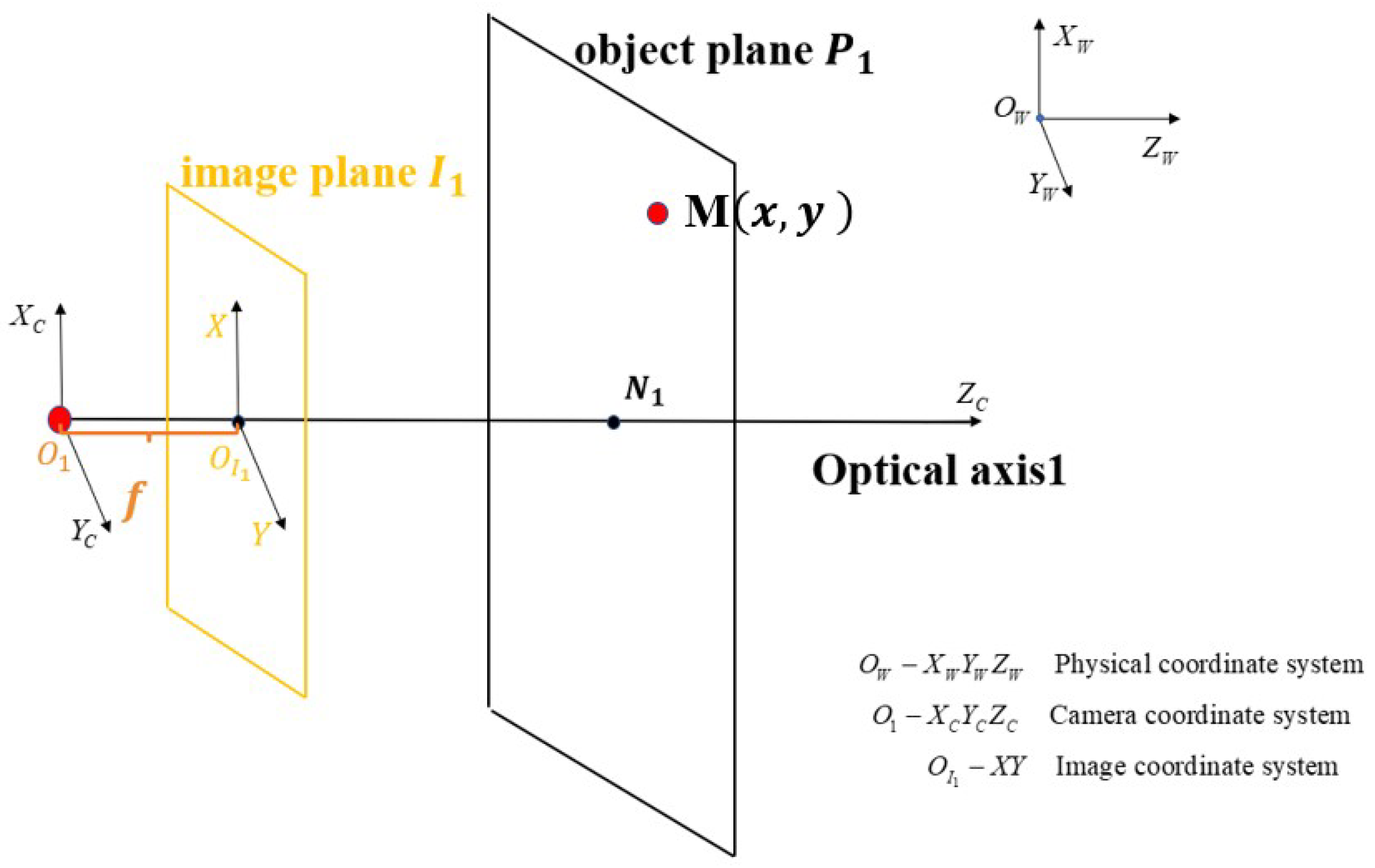
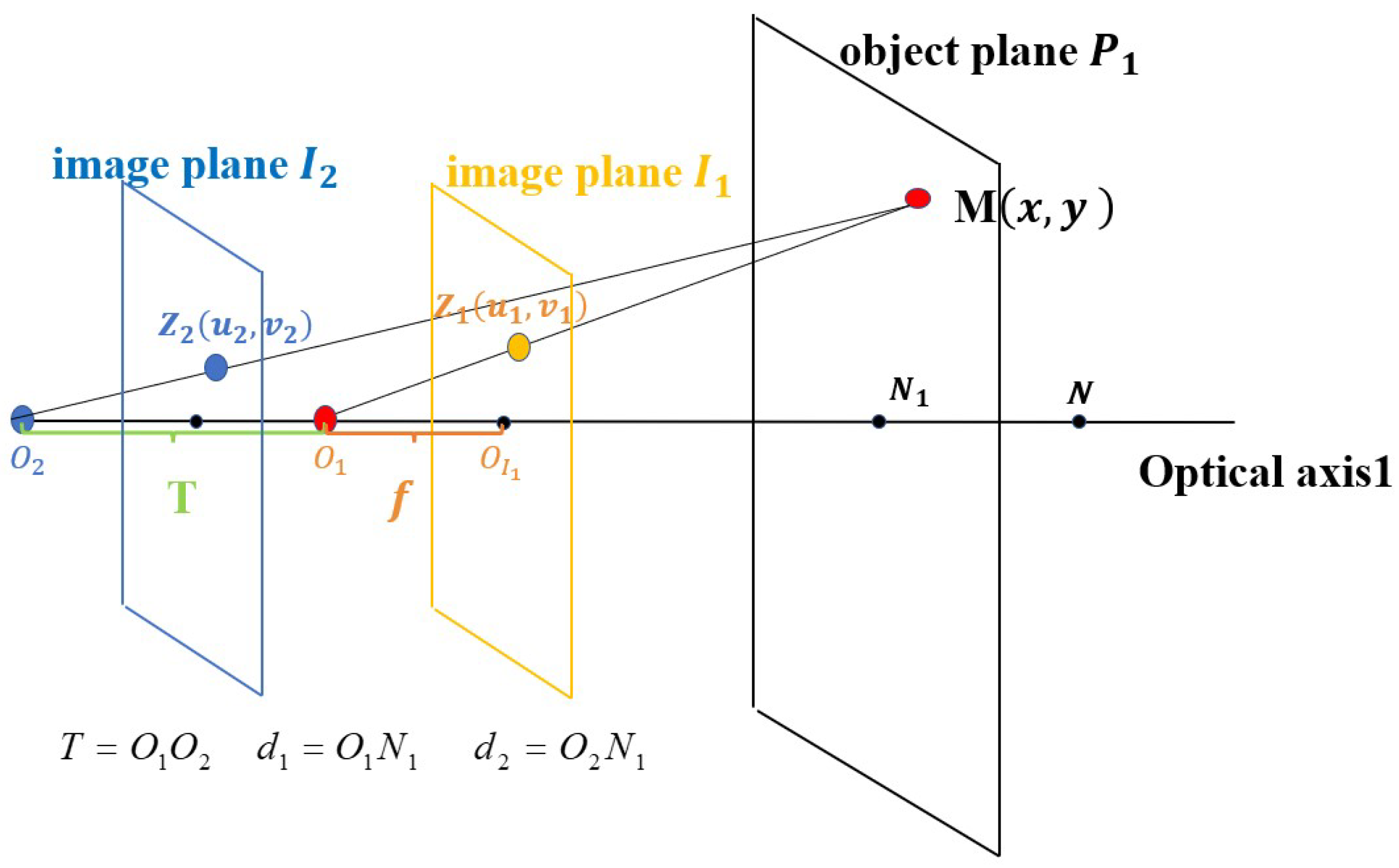
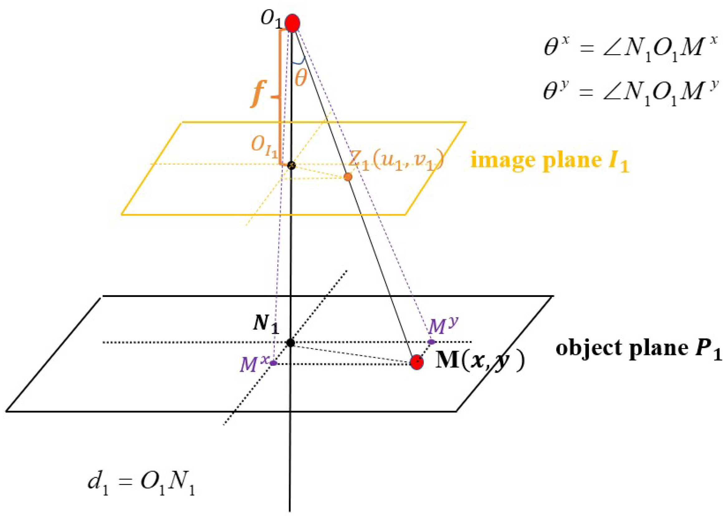
5.1. The Movement of the Camera Center along the Optic Axis

Figure 4 depicts the relationship among the camera, the image planes, the point in the scene, and its projections in image planes when the camera moves along the optic axis. $M=(x,y)$ is the point in the scene with the distance $d_1$ to the camera center $O_1$. $Z_1=\left(u_1,v_1\right)$ is the projection of M on the image plane $I_1$. The three-dimensional coordinate of point M relative to the image plane $I_1$ is $\left(u_1,v_1,d_1\right)$.

When the camera center moves along the optic axis from point $O_1$ to point $O_2$ with distance T and the direction of the optic axis does not change, the new image plane $I_2$ is produced. The projection of M on the image plane $I_2$ is $Z_2=\left(u_2,v_2\right)$, and the depth of M to the camera center changes to $d_2$. The three-dimensional coordinate of the object point M relative to the image plane $I_2$ is changed as $\left(u_2,v_2,d_2\right)$.

The relationship of $Z_1=\left(u_1,v_1\right)$ and $Z_2=\left(u_2,v_2\right)$ is described in the following lemma.

Figure 4. The projection coordinates and related physical quantities corresponding to the object point M when the camera moves along the optical axis with distance T.

Figure 4. The projection coordinates and related physical quantities corresponding to the object point M when the camera moves along the optical axis with distance T.

Lemma 1.

When the camera moves along the optical axis with distance T and the direction of the optic axis does not change, the two projections $Z_1=\left(u_1,v_1\right)$ and $Z_2=\left(u_2,v_2\right)$ of the physical object point $M(x,y)$ before and after the camera movement satisfy the following relationships:

$$\begin{array}{cc}\hfill u_2& =u_1·\frac{d_1}{d_2}=u_1·\frac{d_1}{d_1+T}\hfill \\ \hfill v_2& =v_1·\frac{d_1}{d_2}=v_1·\frac{d_1}{d_1+T}\hfill \end{array}$$

(13)

Proof of Lemma 1.

According to the principle of pinhole optical imaging,

$$\begin{array}{cc}\hfill & u_1=\frac{f_x}{d_1}x\hfill \\ \hfill & u_2=\frac{f_x}{d_2}x\hfill \end{array}$$

(14)

It is easy to find

$$u_2=u_1·\frac{d_1}{d_2}$$

(15)

According to the definition of depth, it is obvious that $d_2=d_1+T$; thus

$$u_2=u_1·\frac{d_1}{d_2}=u_1·\frac{d_1}{d_1+T}.$$

(16)

Similarly, the following relation can be obtained:

$$v_2=v_1·\frac{d_1}{d_2}=v_1·\frac{d_1}{d_1+T}$$

(17)

□

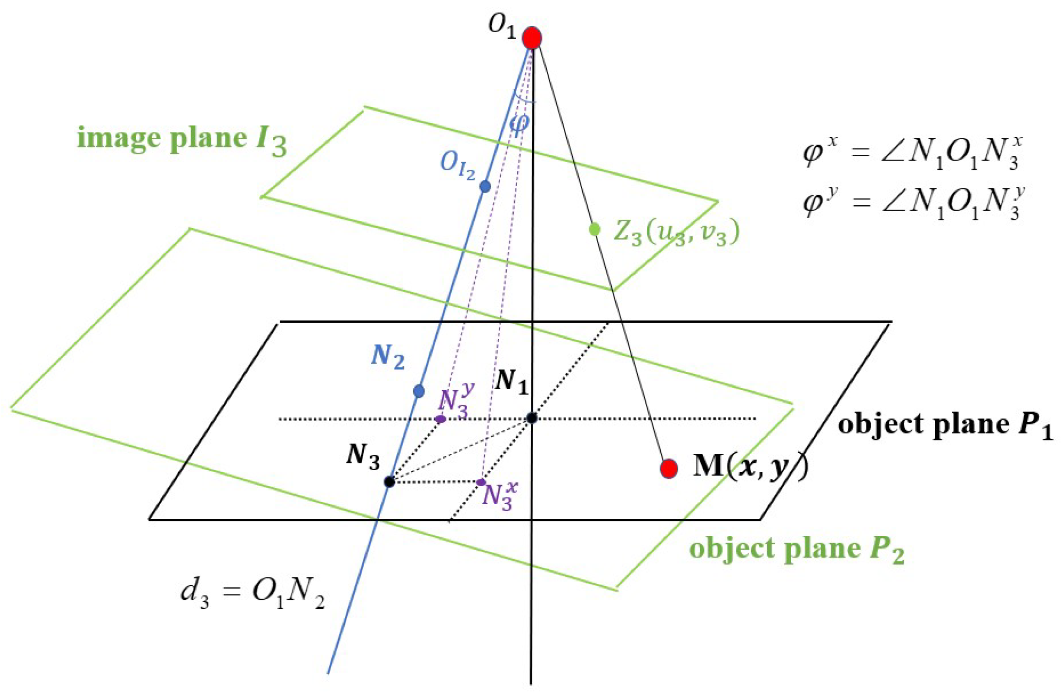
5.2. The Rotation of the Camera’s Optical Axis

The relationship of two image planes produced before and after the rotation of the camera’s optical axis is shown in Figure 5. The camera center position $O_1$ remains unchanged, and the camera optical axis rotates around $O_1$ with an angle $\phi =({\phi }^x,{\phi }^y)$ and produces a new object plane $P_2$ and new image plane $I_3$. The intersection point of the new object plane $P_2$, and the new optical axis is $N_2$.The projection of M on the image plane $I_3$ is $Z_3=\left(u_3,v_3\right)$, and the depth is $d_3$. The three-dimensional coordinate of the object point M relative to the image plane $I_3$ is $\left(u_3,v_3,d_3\right)$.

Lemma 2 gives the relationships among the distance $d_1,d_3$, and the rotation angle $\phi$.

Lemma 2.

If the camera optical axis rotates around the camera center with angle φ while the position of the camera center keeps unchanged, then the two projections $Z_1=\left(u_1,v_1\right)$ and $Z_3=\left(u_3,v_3\right)$ of the physical object point $M(x,y)$ before and after the rotation satisfy the following relationships:

$$d_3=d_1·\frac{cos\left(arctan\frac{u_1}{f_x}-{\phi }^x\right)·cos{\phi }^x}{cos\left(arctan\frac{u_1}{f_x}\right)·cos\phi }=d_1·\frac{cos\left(arctan\frac{v_1}{f_y}-{\phi }^y\right)·cos{\phi }^y}{cos\left(arctan\frac{v_1}{f_y}\right)·cos\phi }$$

(18)

Proof of Lemma 2.

Figure 6 depicts the spatial relationships among the object plane $P_1$, image plane $I_1$, and the optical axis $O_1{N}_1$. In the object plane $P_1$, the points $M^x$ and $M^y$ are the projections of M to the x-axis and y-axis, respectively. Suppose the angle between the initial optical axis $O_1{N}_1$ and the line connecting the object point M and the camera center $P_1$ is $\theta =({\theta }^x,{\theta }^{{}^y})$, where ${\theta }^x=\angle N_1{O}_1{M}^x$, ${\theta }^y=\angle N_1{O}_1{M}^y$.

It is easy to find that,

$$\begin{array}{cc}\hfill & tan{\theta }^x=\frac{|N_1{M}^x|}{|O_1{N}_1|}=\frac{x}{d_1},\hfill \\ \hfill & tan{\theta }^y=\frac{|N_1{M}^y|}{|O_1{N}_1|}=\frac{y}{d_1}\hfill \end{array}$$

(19)

Combine with Formula (14), and we have

$$\begin{array}{cc}\hfill & {\theta }^x=arctan\frac{x}{d_1}=arctan\frac{u_1}{f_x}\hfill \\ \hfill & {\theta }^y=arctan\frac{y}{d_1}=arctan\frac{v_1}{f_y}\hfill \end{array}$$

(20)

When the optical axis rotates around the camera center $O_1$ with angle $\phi ={\phi }^x,{\phi }^y)$, a new object plane $P_2$ and new image plane $I_3$ are produced. Figure 7 depicts the spatial relationships among them. The intersection point of the new object plane $P_2$ and the new optical axis is $N_2$. So, we call the new optical axis $O_1{N}_2$ which passes through the first object plane $P_1$ in the point $N_3$. Figure 8 gives some details of Figure 7. Three points, M, $N_1$, and $N_3$, all locate in the object plane $P_1$, which is depicted in Figure 8a. $N_3^x$ and $N_3^y$ are the projections of $N_3$ to the x- and y-axis in the plane $P_1$; ${\phi }^x=\angle N_1{O}_1{N}_3^x$, ${\phi }^y=\angle N_1{O}_1{N}_3^y$. $\eta =\angle M{O}_1{N}_3=\theta -\phi$.

At the same time, let $N_2^y$ be the projection of $N_2$ to the plane $O_1{N}_1{M}^y$. So, the points $O_1$, $N_1$, $M^y$, $N_2^y$, and $N_3^y$, all fall in the same plane which is depicted in Figure 8b.

Figure 7. The spatial relationships before and after the optical axis rotation with angle $\phi =({\phi }^x,{\phi }^y)$.

Figure 7. The spatial relationships before and after the optical axis rotation with angle $\phi =({\phi }^x,{\phi }^y)$.

Figure 8. Some details of Figure 7: (a) the object plane $P_1$ contains points, M, $N_1$, and $N_3$; (b) the plane contains points $O_1$, $N_1$, $M^y$, $N_2^y$, and $N_3^y$; (c) the plane $O_1{N}_3{N}_3^y$ of (a).

Figure 8. Some details of Figure 7: (a) the object plane $P_1$ contains points, M, $N_1$, and $N_3$; (b) the plane contains points $O_1$, $N_1$, $M^y$, $N_2^y$, and $N_3^y$; (c) the plane $O_1{N}_3{N}_3^y$ of (a).

Considering ${\theta }^y=\angle N_1{O}_1{M}^y$, ${\phi }^y=\angle N_1{O}_1{N}_3^y$ and ${\eta }^y=\angle N_2^y{O}_1{M}^y$ in Figure 8b, respectively, we have

$$\begin{array}{cc}\hfill & cos{\theta }^y=\frac{|O_1{N}_1|}{|O_1{M}^y|}=\frac{d_1}{|O_1{M}^y|},cos{\phi }^y=\frac{|O_1{N}_1|}{|O_1{N}_3^y|}=\frac{d_1}{|O_1{N}_3^y|},cos{\eta }^y=\frac{|O_1{N}_2^y|}{|O_1{M}^y|}\hfill \\ \hfill & \Rightarrow |O_1{N}_2^y|=d_1·\frac{cos{\eta }^y}{cos{\theta }^y},\left|O_1{N}_3^y\right|=d_1·\frac{1}{cos{\phi }^y}\hfill \end{array}$$

(21)

On the other hand, the triangle $O_1{N}_1{N}_3$ in Figure 8a gives the following:

$$cos\phi =\frac{\left|O_1{N}_1\right|}{\left|O_1{N}_3\right|}=\frac{d_1}{\left|O_1{N}_3\right|}\Rightarrow \left|O_1{N}_3\right|=d_1·cos\phi$$

(22)

Figure 8c details the plane $O_1{N}_3{N}_3^y$ of Figure 8a, in which we may find that $\Delta O_1{N}_2{N}_2^y\sim \Delta O_1{N}_3{N}_3^y$, giving the following:

$$\begin{array}{cc}\hfill & \frac{|O_1{N}_2^y|}{|O_1{N}_2|}=\frac{|O_1{N}_3^y|}{|O_1{N}_3|}\hfill \\ \hfill & \Rightarrow \frac{|O_1{N}_2^y|}{d_3}=\frac{|O_1{N}_3^y|}{|O_1{N}_3|}\hfill \\ \hfill & \Rightarrow d_3=\frac{|O_1{N}_3|·|O_1{N}_2^y|}{|O_1{N}_3^y|}\hfill \end{array}$$

(23)

Combining with Equations (21) and (22), we have

$$d_3=d_1·\frac{cos{\eta }^y·cos{\phi }^y}{cos{\theta }^y·cos\phi }$$

(24)

Similarly, we have

$$d_3=d_1·\frac{cos{\eta }^x·cos{\phi }^x}{cos{\theta }^x·cos\phi }$$

(25)

Combining with Equation (20), we have the following results:

$$\Rightarrow \left\{\begin{array}{c}{d}_3=d_1·\frac{cos{\eta }^x·cos{\phi }^x}{cos{\theta }^x·cos\phi }=d_1·\frac{cos\left({\theta }^x-{\phi }^x\right)·cos{\phi }^x}{cos{\theta }^x·cos\phi }=d_1·\frac{cos\left(arctan\frac{u_1}{f_x}-{\phi }^x\right)·cos{\phi }^x}{cos\left(arctan\frac{u_1}{f_x}\right)·cos\phi }\hfill \\ d_3=d_1·\frac{cos{\eta }^y·cos{\phi }^y}{cos{\theta }^y·cos\phi }=d_1·\frac{cos\left({\theta }^y-{\phi }^y\right)·cos{\phi }^y}{cos{\theta }^y·cos\phi }=d_1·\frac{cos\left(arctan\frac{v_1}{f_y}-{\phi }^y\right)·cos{\phi }^y}{cos\left(arctan\frac{v_1}{f_y}\right)·cos\phi }\hfill \end{array}\right.$$

(26)

□

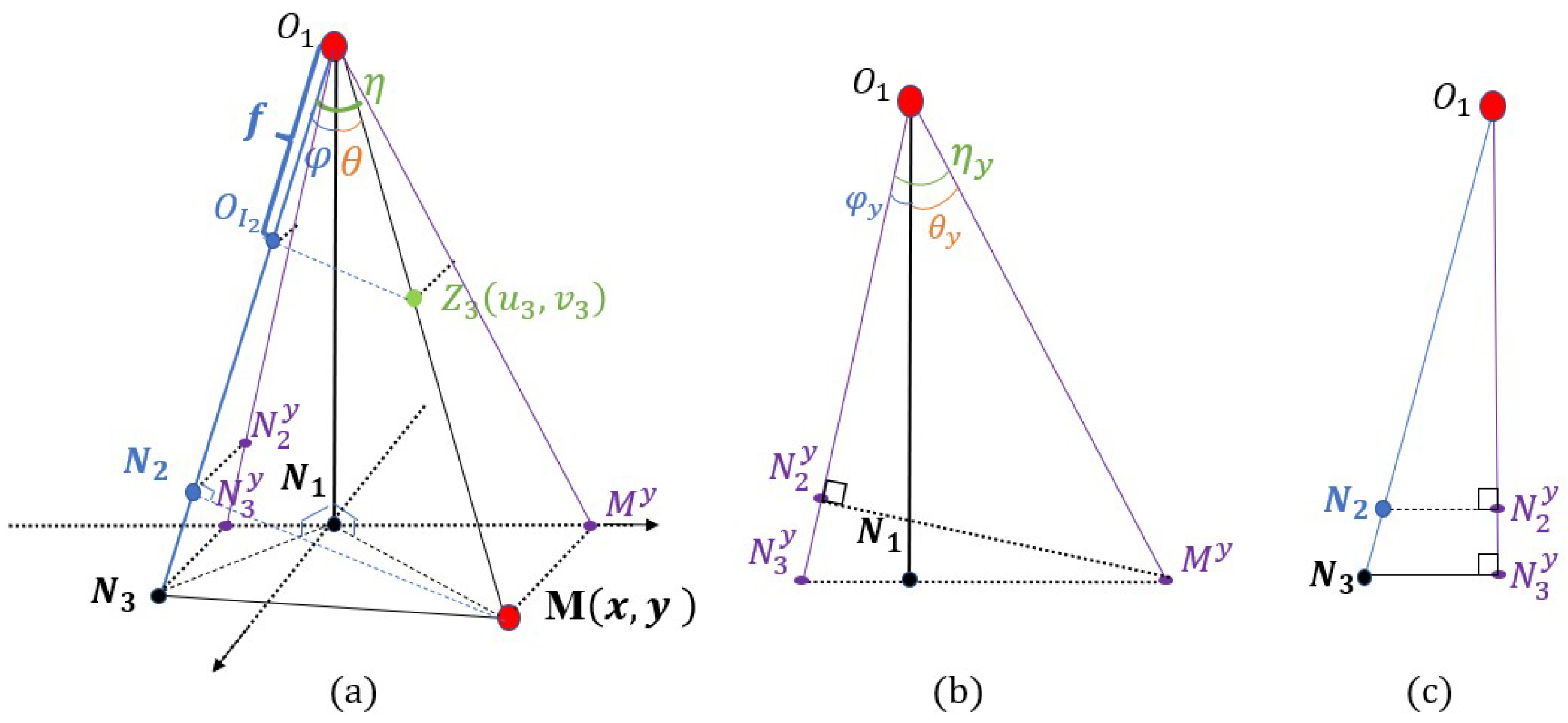
5.3. The Local Property of Depth Information Irrelevant to Camera Movements

Theorem 1.

Assume that the image planes before and after the camera movement are I and $\overline{I}$, respectively, and the corresponding depth functions are d and $bard$, respectively. $Z=(u,v)$ is a keypoint on the image plane I, and $Z^{\prime }=(u^{\prime },v^{\prime })$ is a neighbor pixel of Z in I. The corresponding pixels of Z and $Z^{\prime }$ on the image plane $\overline{I}$ are $\overline{Z}=(\overline{u},\overline{v})$ and ${\overline{Z}}^{\prime }=({\overline{u}}^{\prime },{\overline{v}}^{\prime })$, respectively. Then, the ratio of the depth difference between ${\overline{Z}}^{\prime }$ and $\overline{Z}$ to the depth difference between $Z^{\prime }$ and Z approximates a constant which is irrelevant to $Z^{\prime }$. That is:

$$\frac{\overline{d}\left({\overline{Z}}^{\prime }\right)-\overline{d}\left(\overline{Z}\right)}{d\left(Z^{\prime }\right)-d\left(Z\right)}\approx \alpha$$

(27)

Proof of Theorem 1.

As mentioned before, the camera movement can be decomposed as the movement of the camera center along the optic axis and the rotation of the optic axis around the camera center.

(1) In the first case, Let $I=I_1,\overline{I}=I_2$ according to Lemma 1. We have

$$\begin{array}{cc}\hfill & \overline{d}\left({\overline{Z}}^{\prime }\right)-\overline{d}\left(\overline{Z}\right)=d_2\left({\overline{Z}}^{\prime }\right)-d_2\left(\overline{Z}\right)\hfill \\ \hfill & =\left[d_1\left(Z^{\prime }\right)+T\right]-\left[d_1\left(Z\right)+T\right]\hfill \\ \hfill & =d_1\left(Z^{\prime }\right)-d_1\left(Z\right)=d\left(Z^{\prime }\right)-d\left(Z\right)\hfill \end{array}$$

(28)

(2) In the second case, Let $I=I_1,\overline{I}=I_3$, and according to Lemma 2,

$$\begin{array}{cc}\hfill & \overline{d}\left({\overline{Z}}^{\prime }\right)-\overline{d}\left(\overline{Z}\right)=d_3\left({\overline{Z}}^{\prime }\right)-d_3\left(\overline{Z}\right)\hfill \\ \hfill & =d_1\left(Z^{\prime }\right)·\frac{cos\left(arctan\frac{u^{\prime }}{f_x}-{\phi }^x\right)·cos{\phi }^x}{cos\left(arctan\frac{u^{\prime }}{f_x}\right)·cos\phi }-d_1\left(Z\right)·\frac{cos\left(arctan\frac{u}{f_x}-{\phi }^x\right)·cos{\phi }^x}{cos\left(arctan\frac{u}{f_x}\right)·cos\phi }\hfill \end{array}$$

(29)

Define

$${\beta }_1\triangleq \frac{cos\left(arctan\frac{u}{f_x}-{\phi }^x\right)·cos{\phi }^x}{cos\left(arctan\frac{u}{f_x}\right)·cos\phi }{\beta }_2\triangleq \frac{cos\left(arctan\frac{u^{\prime }}{f_x}-{\phi }^x\right)·cos{\phi }^x}{cos\left(arctan\frac{u^{\prime }}{f_x}\right)·cos\phi }$$

(30)

then

$$\frac{{\beta }_2}{{\beta }_1}=\frac{\frac{cos\left(arctan\frac{u^{\prime }}{f_x}-{\phi }^x\right)·cos{\phi }^x}{cos\left(arctan\frac{u^{\prime }}{f_x}\right)·cos\phi }}{\frac{cos\left(arctan\frac{u}{f_x}-{\phi }^x\right)·cos{\phi }^x}{cos\left(arctan\frac{u}{f_x}\right)·cos\phi }}=\frac{cos\left(arctan\frac{u^{\prime }}{f_x}-{\phi }^x\right)}{cos\left(arctan\frac{u^{\prime }}{f_x}\right)}·\frac{cos\left(arctan\frac{u}{f_x}\right)}{cos\left(arctan\frac{u}{f_x}-{\phi }^x\right)}$$

(31)

By using the Taylor expansion, it can be seen that:

$$\begin{array}{cc}\hfill \frac{{\beta }_2}{{\beta }_1}& =\frac{2-{\left(\frac{u^{\prime }}{f_x}-{\phi }^x\right)}^2}{2-{\left(\frac{u^{\prime }}{f_x}\right)}^2}·\frac{2-{\left(\frac{u}{f_x}\right)}^2}{2-{\left(\frac{u}{f_x}-{\phi }^x\right)}^2}=\frac{2-{\left(\frac{u^{\prime }}{f_x}-{\phi }^x\right)}^2}{2-{\left(\frac{u}{f_x}-{\phi }^x\right)}^2}·\frac{2-{\left(\frac{u}{f_x}\right)}^2}{2-{\left(\frac{u^{\prime }}{f_x}\right)}^2}\hfill \\ \hfill & =\frac{2-{\left(\frac{u}{f_x}-{\phi }^x+\frac{u^{\prime }-u}{f_x}\right)}^2}{2-{\left(\frac{u}{f_x}-{\phi }^x\right)}^2}·\frac{2-{\left(\frac{u}{f_x}\right)}^2}{2-{\left(\frac{u}{f_x}+\frac{u^{\prime }-u}{f_x}\right)}^2}\hfill \end{array}$$

(32)

Because $Z^{\prime }=(u^{\prime },v^{\prime })$ is a neighbor pixel of $Z=(u,v)$, the difference $u^{\prime }-u$ is a small value compared to the optical focal length, that is, $\frac{u^{\prime }-u}{f_x}\ll 1$. So,

$$\frac{2-{\left(\frac{u}{f_x}-{\phi }^x+\frac{u^{\prime }-u}{f_x}\right)}^2}{2-{\left(\frac{u}{f_x}-{\phi }^x\right)}^2}\to 1and\frac{2-{\left(\frac{u}{f_x}\right)}^2}{2-{\left(\frac{u}{f_x}+\frac{u^{\prime }-u}{f_x}\right)}^2}\to 1$$

(33)

thus,

$$\frac{{\beta }_2}{{\beta }_1}\to 1$$

(34)

Then, we have

$$\frac{d_3\left({\overline{Z}}^{\prime }\right)-d_3\left(\overline{Z}\right)}{d_1\left(Z^{\prime }\right)-d_1\left(Z\right)}\approx \frac{cos\left(arctan\frac{u}{f_x}-{\phi }^x\right)·cos{\phi }^x}{cos\left(arctan\frac{u}{f_x}\right)·cos\phi }$$

(35)

It can be seen that the right-hand-side term is relevant to the rotation angle $\phi$ and the position of the keypoint Z but irrelevant to the position of the neighbor pixel $Z^{\prime }$. □

6. Depth-Based Supplemental Vector of the SIFT Feature Descriptor

The image pair I and $\overline{I}$ that needs to be matched can be regarded as the image plane before and after the camera movement. From Theorem 1, the ratio of the depth difference of the keypoint and its neighbor pixels before and after the camera movement is almost a constant. By normalization with the constant, the depth difference is an invariant and can be used as a local feature of the key points.

Select the $n\times n$ neighborhood of the keypoint Z on the image I, and the neighboring pixels are listed as $Z_i^{{}^{\prime }},i=1,\cdots ,n^2-1$. Define

$$\Delta d_i=|d\left(Z_i^{{}^{\prime }}\right)-d\left(Z\right)|,i=1,2,\dots ,n^2-1$$

(36)

$$d^{*}=\underset{i}{min}\left\{\Delta d_i|\Delta d_i\ne 0\right\}$$

(37)

$$\Delta D=\left\{\begin{array}{c}0,ifd*=0\hfill \\ (\frac{\Delta d_1}{d^{*}},\frac{\Delta d_2}{d^{*}},\dots ,\frac{\Delta d_{n^2-1}}{d^{*}}),else\hfill \end{array}\right.$$

(38)

The vector $\Delta D$ is the depth-based local feature information, which can be used as a supplement to the SIFT feature descriptor. The properties of the theorem can be applied not only to SIFT, but also to other methods, such as SURF.

7. Experiments

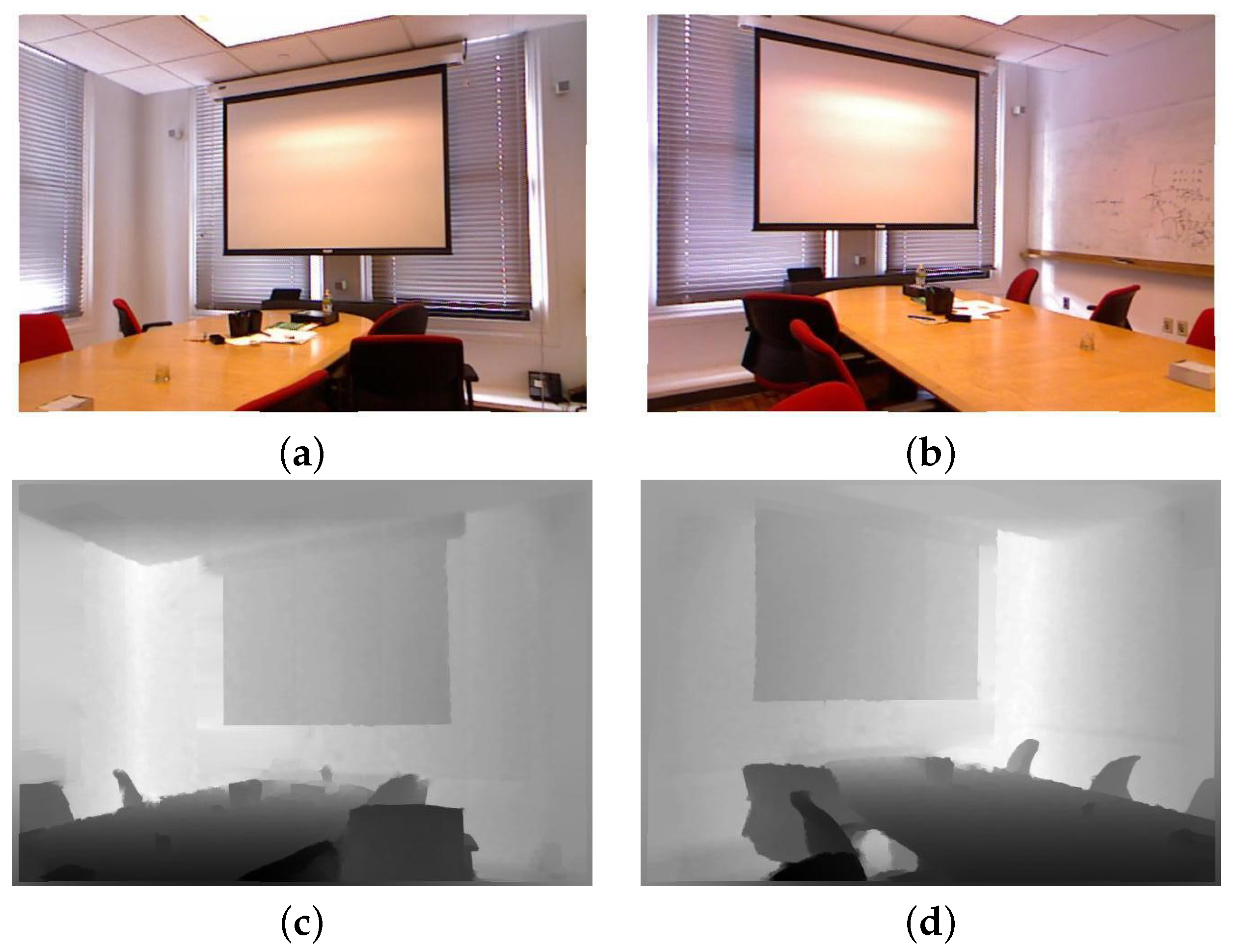
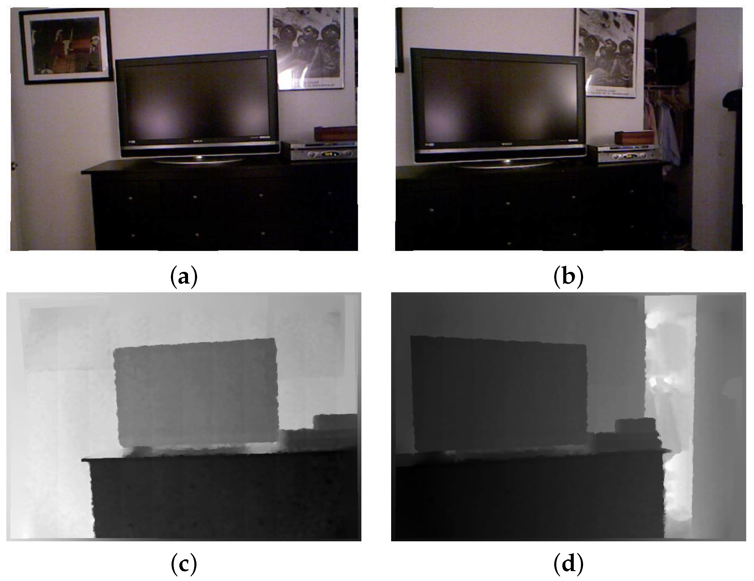
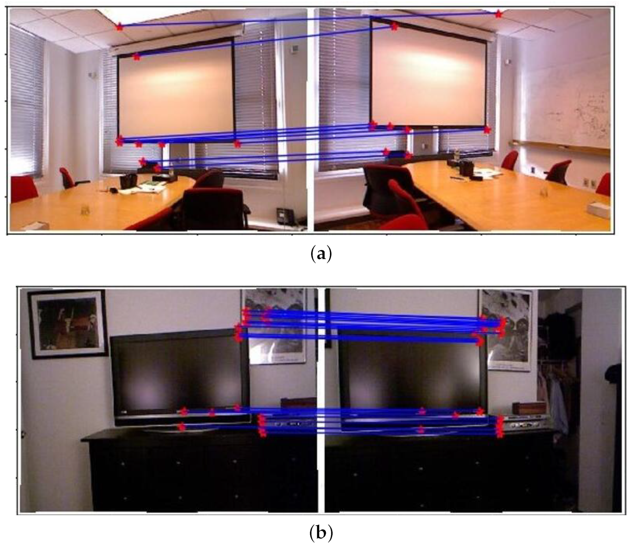
7.1. Experimental Data

The experimental images are taken from the NYU dataset [47] which has a total of 1449 indoor scene RGB images and corresponding depth images with size of 640 × 480. In this paper, 20 images were selected to form 10 pairs for experimental comparison. We show the results of the second pair (numbered 25 and 26 in the database) and the sixth pair (numbered 191 and 192 in the database).

The experiments were performed under a Windows 10 operating system, using the Python-Open CV computer vision library for image processing.

Figure 9 and Figure 10 show the original RGB image pairs and the corresponding depth images. Figure 9a and Figure 9b correspond to the RGB images numbered 25 and 26 in the database, respectively. Figure 9c and Figure 9d are depth images of Figure 9a and Figure 9b, respectively. Figure 10a and Figure 10b correspond to the RGB images of numbered 191 and 192 in the database, respectively. Figure 10c and Figure 10d are depth images of Figure 10a and Figure 10b, respectively.

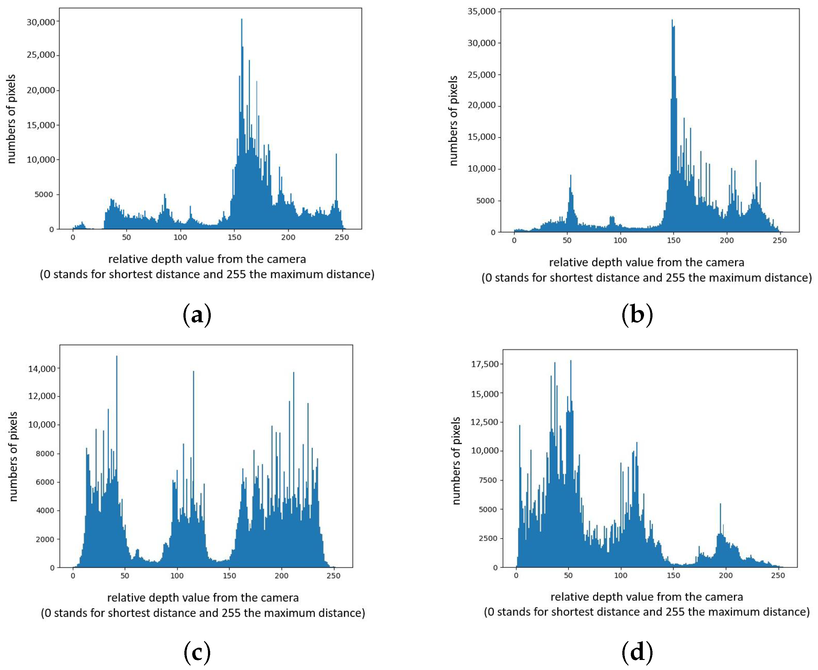
7.2. Pixel Pre-Classification

Figure 11 presents the depth information histograms of Figure 9c,d and Figure 10c,d. It is observed that each histogram can be roughly considered to have three peaks, that is, the objects in the image roughly are classified as falling in the foreground, middle ground, or background. Accordingly, the pixels of the RGB image are divided into three categories corresponding to the depth information. This paper simply uses 30% and 70% of the cumulative frequency as the threshold.

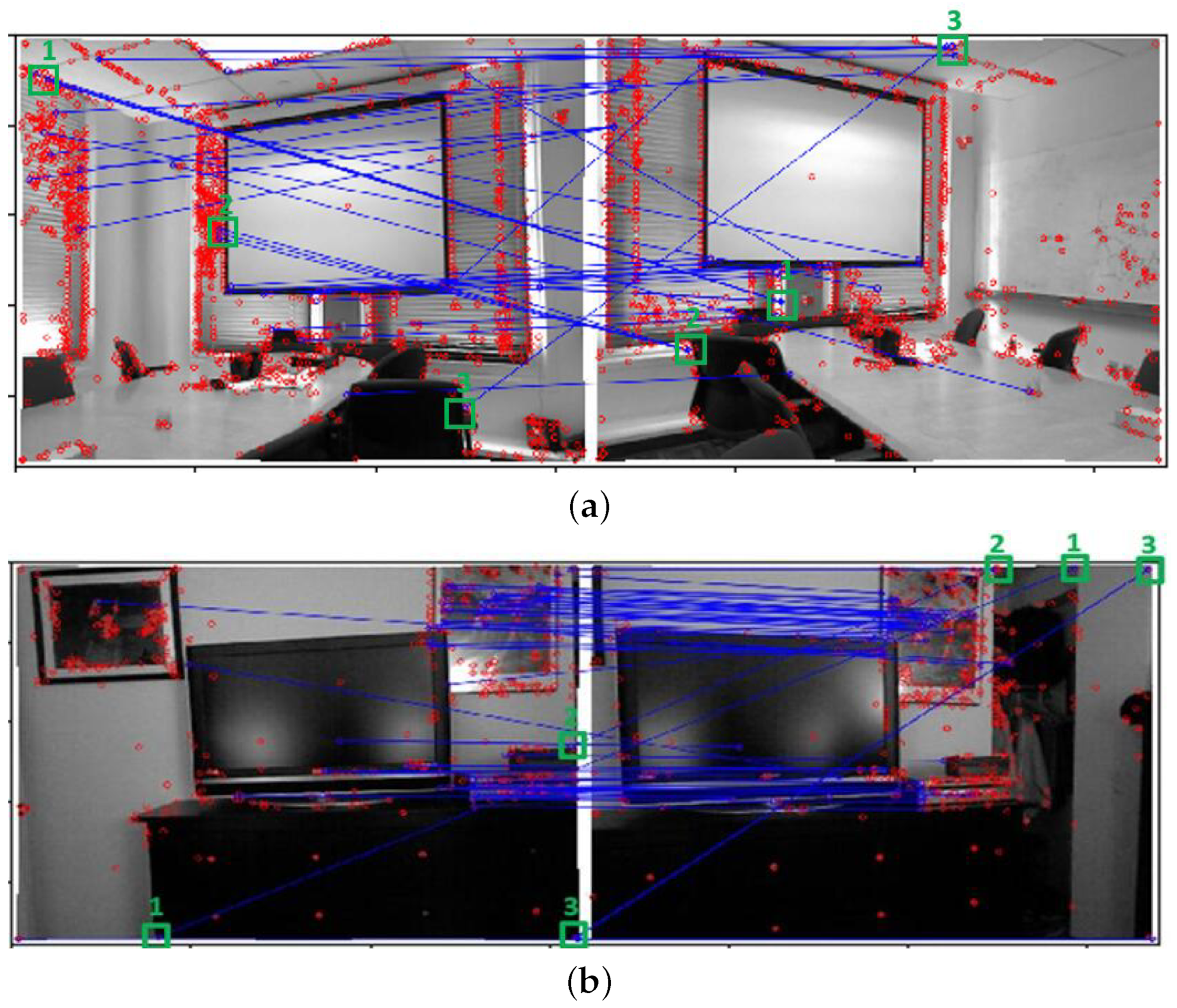
7.3. Experimental Results

We use the SIFT algorithm to extract image keypoint features and use the Kd-tree algorithm [24] to perform keypoint feature matching. The results are shown in Figure 12. Figure 12a is the matching result of the SIFT algorithm in Figure 9a,b, and Figure 12b is the matching result of the SIFT algorithm in Figure 10a,b.

It can be seen from Figure 12 that there are many false matching pairs in the results of SIFT matching. For example, in Figure 12a, the keypoint pair 1 marked by the green box is located at the coordinates (46, 54) in the left image which is on the ceiling; however, in the right image, the corresponding coordinates (212, 297) are located at the bottom of the screen. Obviously, this is not the same object point. Similarly, the other green box matching point pairs are false matches.

In this paper, the SIFT algorithm is used to obtain the keypoints first, the SIFT descriptor combining with a depth-information supplemental vector is constructed as the new descriptor for matching, and the Kd-tree algorithm is used to match the similar keypoints in the image pair.

Figure 13 presents the improved matching results for the second and sixth image pairs. It can be seen that the keypoint pairs that were originally incorrectly matched have been removed.

Table 1. Comparison of image pair matching before and after improvement.

Image Pair	Total Number of Keypoints	Number of SIFT Matching Pairs	Accuracy Rate	Number of Matching Pairs after Improvement	Accuracy Rate
1(18,19)	629	28	67.86%	14	78.57%
2(25,26)	2756	41	36.59%	9	88.89%
3(69,70)	2038	28	96.43%	13	100.00%
4(124,125)	2800	514	77.43%	375	90.13%
5(131,132)	2424	378	89.15%	280	96.43%
6(191,192)	1101	66	80.30%	22	100.00%
7(411,412)	1282	46	89.13%	19	94.74%
8(510,511)	1065	39	84.62%	16	93.75%
9(568,569)	2238	84	83.33%	43	93.02%
10(975,976)	1681	52	82.69%	24	91.67%

gives the comparison of the matching results of all ten pairs of images.

From Table 1, we can see that the method proposed in this paper can effectively filter out the wrong matching point pairs, and the accuracy rate of image pair matching has been significantly improved. The accuracy rate has been increased by an average of 13.967 percentage points. Since the relative depth information is used, there is no specific requirement about the accuracy of the depth information. In practice, an estimated depth without a scale factor or an approximate dense depth map can be used.

8. Conclusions

In this paper, we analyzed the local property of the depth information of image pairs taken before and after camera movements and proved that the ratio of the depth difference of a keypoint and its neighbor pixels before and after the camera movement approximates a constant. Based on this property, a depth-based feature vector was constructed as a supplement of SIFT feature descriptor. All the keypoints were classified as foreground, middle ground, and background and the feature matching was performed within the same class.

Experiments were performed to validate the effectiveness of the proposed method. The experimental images were taken from the NYU dataset. total of 20 images were selected to form 10 pairs for experimental comparison. The experimental results show that the accuracy rate of image pair matching increased by an average of 13.967 percentage points, which means the method proposed in this paper can effectively filter out mismatch point pairs.

The local property described in the theorem proposed in this paper is a common feature which may be used for other situations, not only for a supplement of the SIFT feature descriptor and can be widely used in all aspects of image matching. The relative depth differences used for the local property do not require accurate depth information. In addition, we intend to further optimize the related model of image stitching according to the proposed method.

References

1. Ma, J.; Jiang, X.; Fan, A.; Jiang, J.; Yan, J. Image Matching from Handcrafted to Deep Features: A Survey. Int. J. Comput. Vis. 2020, 1, 23–79. [Google Scholar] [CrossRef]
2. Zitová, B.; Flusser, J. Image Registration Methods: A Survey. Image Vis. Comput. 2003, 21, 977–1000. [Google Scholar] [CrossRef] [Green Version]
3. Lowe, D.G. Distinctive Image Features from Scale-Invariant Keypoints. Int. J. Comput. Vis. 2004, 60, 91–110. [Google Scholar] [CrossRef]
4. Bay, H.; Tuytelaars, T.; Gool, L.V. SURF: Speeded up robust features. In Proceedings of the 9th European Conference on Computer Vision, Graz, Austria, 7–13 May 2006. [Google Scholar]
5. Alahi, A.; Ortiz, R.; Vandergheynst, P. FREAK: Fast Retina Keypoint. In Proceedings of the 2012 IEEE Conference on Computer Vision and Pattern Recognition, Providence, RI, USA, 16–21 June 2012. [Google Scholar]
6. Bellavia, F. SIFT Matching by Context Exposed. IEEE Trans. Pattern Anal. Mach. Intell. 2022, 45, 2445–2457. [Google Scholar] [CrossRef] [PubMed]
7. Liu, W.; Wang, Y.; Chen, J.; Guo, J.; Lu, Y. A completely affine invariant image-matching method based on perspective projection. Mach. Vis. Appl. 2012, 23, 231–242. [Google Scholar] [CrossRef]
8. Mishkin, D.; Matas, J.; Perdoch, M. MODS: Fast and robust method for two-view matching. Comput. Vis. Image Underst. 2015, 141, 81–93. [Google Scholar] [CrossRef] [Green Version]
9. Morel, J.M.; Yu, G. Asift: A new framework for fully affine invariant image comparison. SIAM J. Imaging Sci. 2009, 2, 438–469. [Google Scholar] [CrossRef] [Green Version]
10. Pang, Y.; Li, W.; Yuan, Y.; Pan, J. Fully affine invariant surf for image matching. Neurocomputing 2012, 85, 6–10. [Google Scholar] [CrossRef]
11. Toft, C.; Turmukhambetov, D.; Sattler, T.; Kahl, F.; Brostow, G.J. Single-Image Depth Prediction Makes Feature Matching Easier. In Proceedings of the Computer Vision—ECCV 2020: 16th European Conference, Glasgow, UK, 23–28 August 2020. [Google Scholar]
12. Chen, Y.; Wang, G.; Wu, L. Research on feature point matching algorithm improvement using depth prediction. J. Eng. 2019, 2019, 8905–8909. [Google Scholar] [CrossRef]
13. Schuon, S.; Theobalt, C.; Davis, J.; Thrun, S. LidarBoost: Depth superresolution for ToF 3D shape scanning. In Proceedings of the 2009 IEEE Conference on Computer Vision and Pattern Recognition, Miami, FL, USA, 20–25 June 2009; pp. 343–350. [Google Scholar]
14. Liu, C.; Kim, K.; Gu, J.; Furukawa, Y.; Kautz, J. Planercnn: 3d plane detection and reconstruction from a single image. In Proceedings of the IEEE Conference on Computer Vision and Pattern Recognition, Long Beach, CA, USA, 15–20 June 2019; pp. 4450–4459. [Google Scholar]
15. Liu, C.; Yang, J.; Ceylan, D.; Yumer, E.; Furukawa, Y. Planenet: Piece-wise planar reconstruction from a single rgb image. In Proceedings of the IEEE Conference on Computer Vision and Pattern Recognition, Salt Lake City, UT, USA, 18–22 June 2018; pp. 2579–2588. [Google Scholar]
16. Li, Z.; Snavely, N. Megadepth: Learning single-view depth prediction from internet photos. In Proceedings of the IEEE Conference on Computer Vision and Pattern Recognition, Salt Lake City, UT, USA, 18–22 June 2018. [Google Scholar]
17. Li, J.; He, L.; Ren, G. A feature point matching method for binocular stereo vision images based on deep learning. Autom. Instrum. 2022, 2, 57–60. [Google Scholar]
18. Zhang, Z.; Huo, W.; Lian, M.; Yang, L. Research on fast binocular stereo vision ranging based on Yolov5. J. Qingdao Univ. Eng. Technol. Ed. 2021, 36, 20–27. [Google Scholar]
19. Chen, W.; Fu, Z.; Yang, D.; Deng, J. Single-image depth perception in the wild. In Proceedings of the 30th International Conference on Neural Information Processing Systems, Barcelona, Spain, 5–10 December 2016; pp. 730–738. [Google Scholar]
20. Ummenhofer, B.; Zhou, H.; Uhrig, J.; Mayer, N.; Ilg, E.; Dosovitskiy, A.; Brox, T. DeMoN: Depth and Motion Network for Learning Monocular Stereo. In Proceedings of the IEEE Conference on Computer Vision and Pattern Recognition (CVPR), Honolulu, HI, USA, 21–26 July 2017. [Google Scholar]
21. Facil, J.M.; Ummenhofer, B.; Zhou, H.; Montesano, L.; Brox, T.; Civera, J. CAM-Convs: Camera-Aware Multi-Scale Convolutions for Single-View Depth. In Proceedings of the 2019 IEEE/CVF Conference on Computer Vision and Pattern Recognition (CVPR), Long Beach, CA, USA, 15–20 June 2019. [Google Scholar]
22. Zhou, H.; Ummenhofer, B.; Brox, T. DeepTAM: Deep Tracking and Mapping with Convolutional Neural Networks. Int. J. Comput. Vis. 2020, 128, 756–769. [Google Scholar] [CrossRef]
23. Silberman, N.; Hoiem, D.; Kohli, P.; Fergus, R. Indoor Segmentation and Support Inference from RGBD Images; Springer: Berlin/Heidelberg, Germany, 2012. [Google Scholar]
24. Abdel-Hakim, A.E.; Farag, A. CSIFT: A SIFT Descriptor with Color Invariant Characteristics. In Proceedings of the IEEE Computer Society Conference on Computer Vision Pattern Recognition, New York, NY, USA, 17–22 June 2006. [Google Scholar]
25. Rublee, E.; Rabaud, V.; Konolige, K.; Bradski, G. ORB: An efficient alternative to SIFT or SURF. In Proceedings of the 2011 International Conference on Computer Vision, Barcelona, Spain, 6–13 November 2011; pp. 2564–2571. [Google Scholar]
26. Rosten, E.; Porter, R.; Drummond, T. Faster and better: A machine learning approach to corner detection. IEEE Trans. Pattern Anal. Mach. Intell. 2010, 32, 105–119. [Google Scholar] [CrossRef] [Green Version]
27. Calonder, M.; Lepetit, V.; Strecha, C.; Fua, P. Brief: Binary robust independent elementary features. In Proceedings of the European Conference on Computer Vision, Crete, Greece, 5–11 September 2010; pp. 778–792. [Google Scholar]
28. Balammal Geetha, S.; Muthukkumar, R.; Seenivasagam, V. Enhancing Scalability of Image Retrieval Using Visual Fusion of Feature Descriptors. Intell. Autom. Soft Comput. 2022, 31, 1737–1752. [Google Scholar] [CrossRef]
29. Csurka, G.; Dance, R.; Fan, L.; Willamowski, J.; Bray, C. Visual categorization with bags of keypoints. In Proceedings of the Workshop on Statistical Learning in Computer Vision, Prague, Czech Republic, May 2004; pp. 1–22. [Google Scholar]
30. Tang, L.; Ma, S.; Ma, X.; You, H. Research on Image Matching of Improved SIFT Algorithm Based on Stability Factor and Feature Descriptor Simplification. Appl. Sci. 2022, 12, 8448. [Google Scholar] [CrossRef]
31. Feng, Q.; Tao, S.; Liu, C.; Qu, H.; Xu, W. IFRAD: A Fast Feature Descriptor for Remote Sensing Images. Remote Sens. 2021, 13, 3774. [Google Scholar] [CrossRef]
32. Fischler, M.A.; Bolles, R.C. Random Sample Consensus: A Paradigm for Model Fitting with Applications to Image Analysis and Automated Cartography. Commun. ACM 1981, 24, 381–395. [Google Scholar] [CrossRef]
33. Chung, K.L.; Tseng, Y.C.; Chen, H.Y. A Novel and Effective Cooperative RANSAC Image Matching Method Using Geometry Histogram-Based Constructed Reduced Correspondence Set. Remote Sens. 2022, 14, 3256. [Google Scholar] [CrossRef]
34. Tombari, F.; Salti, S.; Stefano, L.D. Unique signatures of histograms for local surface description. In Proceedings of the European Conference on Computer Vision, Crete, Greece, 5–11 September 2010; pp. 356–369. [Google Scholar]
35. Salti, S.; Tombari, F.; Di Stefano, L. SHOT: Unique Signatures of Histograms for Surface and Texture Description. Comput. Vis. Image Underst. 2014, 125, 251–264. [Google Scholar] [CrossRef]
36. Prakhya, S.M.; Liu, B.; Lin, W. B-SHOT: A binary feature descriptor for fast and efficient keypoint matching on 3D point clouds. In Proceedings of the 2015 IEEE/RSJ International Conference on Intelligent Robots and Systems (IROS), Hamburg, Germany, 28 September–2 October 2015; pp. 1929–1934. [Google Scholar]
37. Steder, B.; Rusu, R.B.; Konolige, K.; Burgard, W. NARF: 3D range image features for object recognition. In Proceedings of the International Conference on Intelligent Robots and Systems (IROS), Taipei, Taiwan, 18–22 October 2010. [Google Scholar]
38. Johnston, A.; Carneiro, G. Self-supervised monocular trained depth estimation using self-attention and discrete disparity volume. In Proceedings of the IEEE/CVF Conference on Computer Vision and Pattern Recognition (CVPR), Seattle, WA, USA, 13–19 June 2020. [Google Scholar]
39. Zhou, T.; Brown, M.; Snavely, N.; Lowe, D.G. Unsupervised learning of depth and ego-motion from video. In Proceedings of the IEEE/CVF Conference on Computer Vision and Pattern Recognition (CVPR), Honolulu, HI, USA, 21–26 July 2017; pp. 21–26. [Google Scholar]
40. Ranjan, A.; Jampani, V.; Balles, L.; Kim, K.; Sun, D.; Wulff, J.; Black, M.J. Competitive collaboration: Joint unsupervised learning of depth, camera motion, optical flow and motion segmentation. In Proceedings of the IEEE/CVF Conference on Computer Vision and Pattern Recognition (CVPR), Long Beach, CA, USA, 15–20 June 2019; pp. 15–20. [Google Scholar]
41. Mahjourian, R.; Wicke, M.; Angelova, A. Unsupervised Learning of Depth and Ego-Motion from Monocular Video Using 3D Geometric Constraints. In Proceedings of the 2018 IEEE/CVF Conference on Computer Vision and Pattern Recognition (CVPR), Salt Lake City, UT, USA, 18–22 June 2018; pp. 5667–5675. [Google Scholar]
42. Wang, J.; Liu, P.; Wen, F. Self-supervised learning for RGB-guided depth enhancement by exploiting the dependency between RGB and depth. IEEE Trans. Image Process. 2023, 32, 159–174. [Google Scholar] [CrossRef]
43. Marr, D.; Hildreth, E. Theory of Edge Detection. Proc. R. Soc. Biol. Sci. 1980, 207, 187–217. [Google Scholar]
44. Olkkonen, H.; Pesola, P. Gaussian Pyramid Wavelet Transform for Multiresolution Analysis of Images. Graph. Model. Image Process. 1996, 58, 394–398. [Google Scholar] [CrossRef]
45. Lindeberg, T. Feature Detection with Automatic Scale Selection. Int. J. Comput. Vis. 1998, 30, 79–116. [Google Scholar] [CrossRef]
46. Wang, M.; Lai, C.H. A Concise Introduction to Image Processing using C++; Chapman and Hall/CRC: Boca Raton, FL, USA, 2009. [Google Scholar]
47. Ram, P.; Sinha, K. Revisiting kd-tree for nearest neighbor search. In Proceedings of the 25th Acm Sigkdd International Conference on Knowledge Discovery & Data Mining, Anchorage, AK, USA, 4–8 August 2019; pp. 1378–1388. [Google Scholar]
Figure 1. The discretization of the gradient direction.
Mathematics 11 01154 g001
Figure 2. Mismatching results of the traditional SIFT algorithm (keypoint pairs 1, 2, and 3 marked in green boxes).
Mathematics 11 01154 g002
Figure 3. The relationship among three coordinates.
Mathematics 11 01154 g003
Figure 5. Projection coordinates and related physical quantities corresponding to the object point M when the optical axis rotates with angle φ .
Mathematics 11 01154 g005
Figure 6. The spatial relationships among the object plane P 1 , image plane I 1 , and the optical axis O 1 N 1 .
Mathematics 11 01154 g006
Figure 9. The RGB image of the second pair and their depth images: (a) original RGB image numbered 25; (b) original RGB image numbered 26; (c) depth image of (a); (d) depth image of (b).
Mathematics 11 01154 g009
Figure 10. The RGB image of the sixth pair and their depth images: (a) original RGB image numbered 191; (b) original RGB image numbered 192; (c) depth image of (a); (d) depth image of (b).
Mathematics 11 01154 g010
Figure 11. Image pair depth information histogram: (a) depth information histogram of image No. 25; (b) depth information histogram of image No. 26; (c) depth information histogram of image No. 191; (d) depth information histogram of image No. 192.
Mathematics 11 01154 g011
Figure 12. SIFT algorithm matching results: (a) Figure 9a,b matching result of SIFT algorithm; (b) Figure 10a,b matching result of SIFT algorithm.
Mathematics 11 01154 g012
Figure 13. Matching results of the improved algorithm: (a) Figure 8a,b matching results of the improved algorithm; (b) Figure 9a,b matching results of the improved algorithm.
Mathematics 11 01154 g013