
Fuzzy Portfolio Selection in the Risk Attitudes of Dimension Analysis under the Adjustable Security Proportions


Abstract
1. Introduction
2. Preliminaries
- (1)
- The fuzzy number is normal, if there exists an x ∈ R with ;
- (2)
- is convex, i.e., (λx + (1 − λ)y) ≥ min{(x), (y)}, ∀ x, y∈ R and λ ∈ [0, 1];
- (3)
- is upper semicontinuous, i.e., { x ∈ R:(x) ≥ α} = is a closed subset of U for each α ∈ (0, 1];
- (4)
- The closure of the set { x ∈ R:(x) ≥ 0} is a compact subset of R.
3. The Dimension Risk Analysis in Adjustable Security Proportions
4. Illustrations
4.1. Data Description and Model Explanation
4.2. Results and Discussions
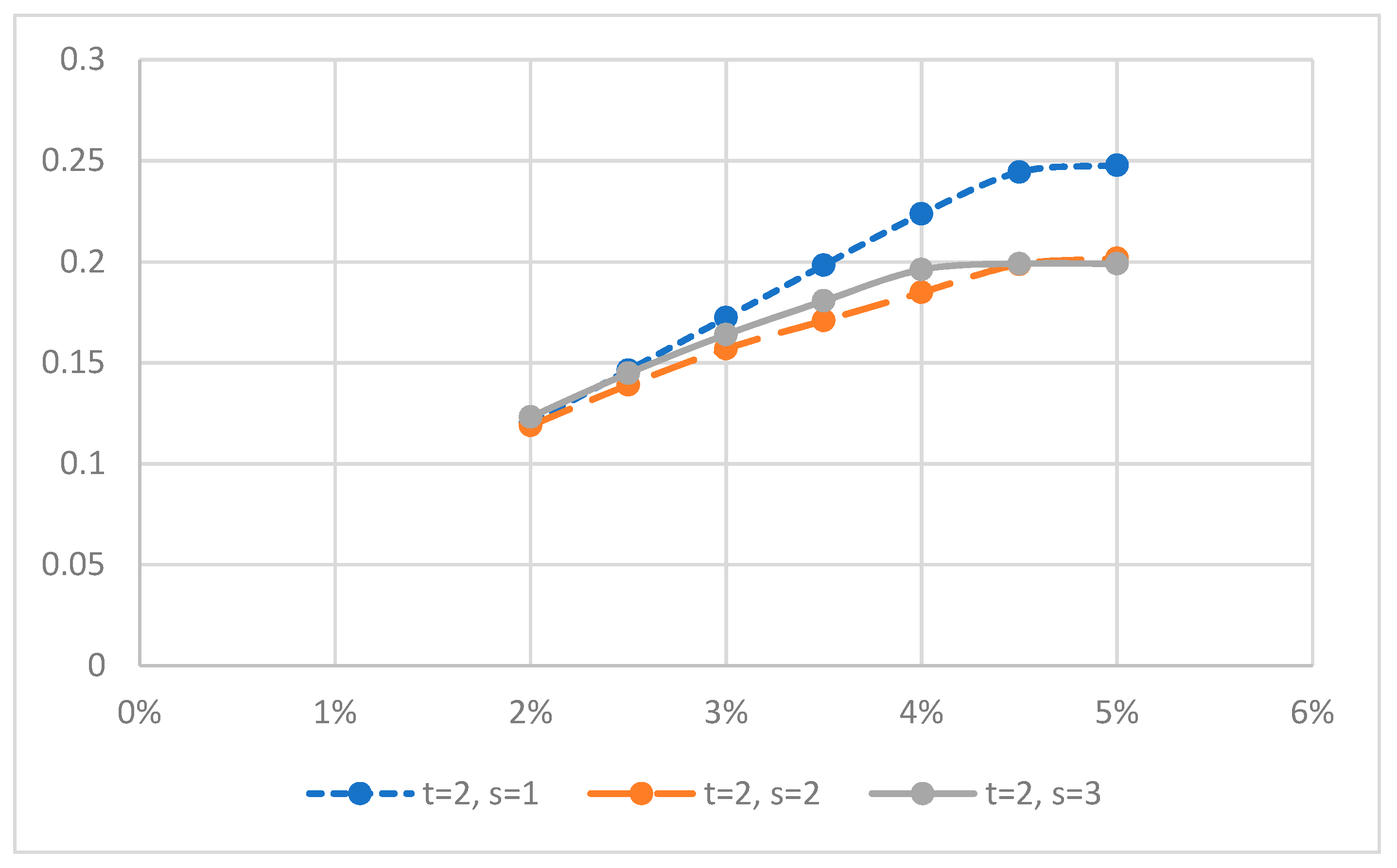
4.2.1. Experiment 1
4.2.2. Experiment 2
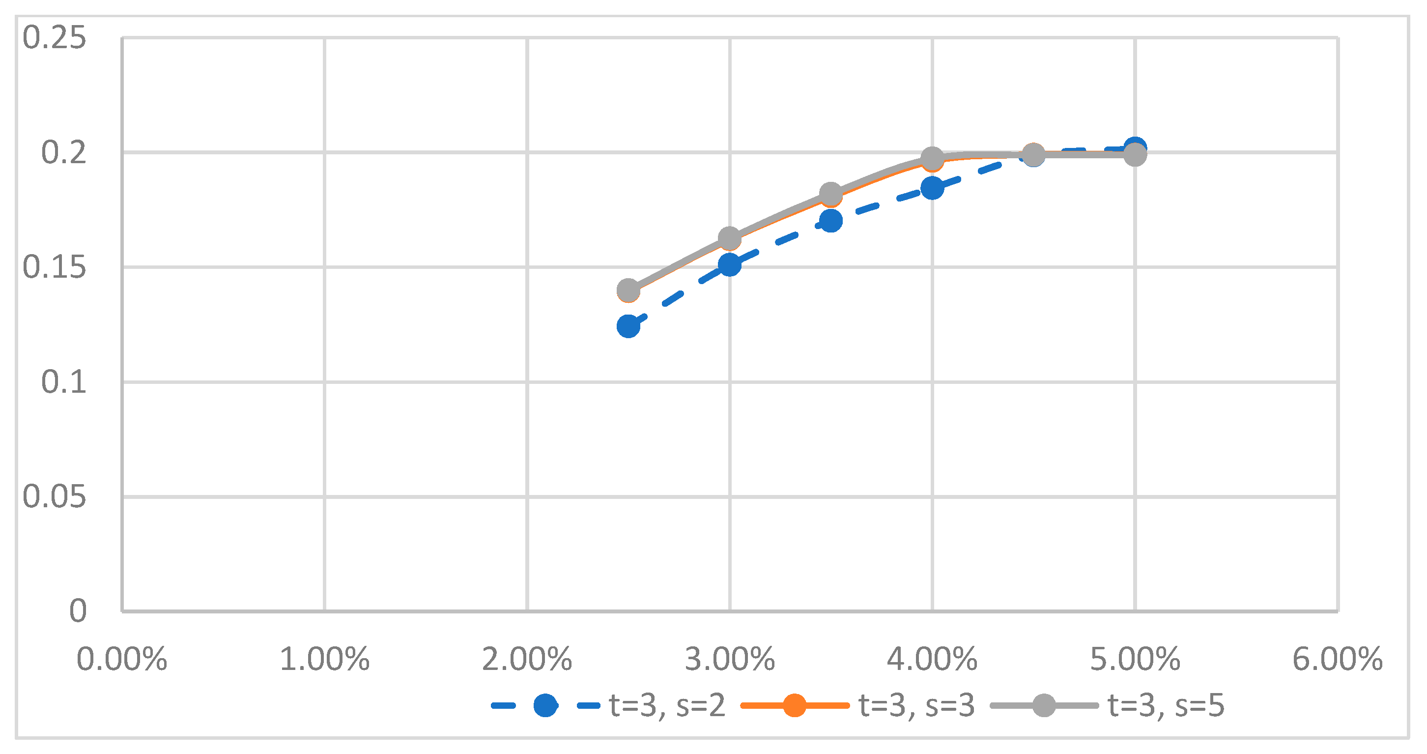
4.2.3. Experiment 3
5. Conclusions
Author Contributions
Funding
Institutional Review Board Statement
Informed Consent Statement
Data Availability Statement
Acknowledgments
Conflicts of Interest
References
- Markowitz, H. Portfolio selection. J. Financ. 1952, 7, 77–91. [Google Scholar]
- Sharpe, W.F. Portfolio Theory and Capital Markets; McGraw-Hill: New York, NY, USA, 1970. [Google Scholar]
- Merton, R.C. An analytic derivation of the efficient frontier. J. Financ. Quant. Anal. 1972, 10, 1851–1872. [Google Scholar] [CrossRef]
- Pang, J.S. A new efficient algorithm for a class of portfolio selection problems. Oper. Res. 1980, 28, 754–767. [Google Scholar] [CrossRef]
- Perold, A.F. Large-scale portfolio optimization. Manag. Sci. 1984, 30, 1143–1160. [Google Scholar] [CrossRef]
- Vörös, J. Portfolio analysis—An analytic derivation of the efficient portfolio frontier. Eur. J. Oper. Res. 1990, 203, 294–300. [Google Scholar] [CrossRef]
- Best, M.J.; Grauer, R.R. The efficient set mathematics when mean–variance problems are subject to general linear constrains. J. Econ. Bus. 1990, 42, 105–120. [Google Scholar] [CrossRef]
- Best, M.J.; Hlouskova, J. The efficient frontier for bounded assets. Math. Method Oper. Res. 2000, 52, 195–212. [Google Scholar] [CrossRef]
- Gupta, P.; Mehlawat, M.K.; Yadav, S.; Kumar, A. A polynomial goal programming approach for intuitionistic fuzzy portfolio optimization using entropy and higher moments. Appl. Soft Comput. 2019, 85, 105781. [Google Scholar] [CrossRef]
- Wu, Y.; Xu, C.; Ke, Y.; Tao, Y.; Li, X. Portfolio optimization of renewable energy projects under type-2 fuzzy environment with sustainability perspective. Comput. Ind. Eng. 2019, 133, 69–82. [Google Scholar] [CrossRef]
- Mansour, N.; Cherif, M.S.; Abdelfattah, W. Multi-objective imprecise programming for financial portfolio selection with fuzzy returns. Expert Syst. Appl. 2019, 138, 112810. [Google Scholar] [CrossRef]
- Yue, W.; Wang, Y.; Xuan, H. Fuzzy multi-objective portfolio model based on semi-variance–semi-absolute deviation risk measures. Soft Comput. 2019, 23, 8159–8179. [Google Scholar] [CrossRef]
- Liagkouras, K.; Metaxiotis, K. Multi-period mean–variance fuzzy portfolio optimization model with transaction costs. Eng. Appl. Artif. Intell. 2018, 67, 260–269. [Google Scholar] [CrossRef]
- Gupta, P.; Mehlawat, M.K.; Khan, A.Z. Multi-period portfolio optimization using coherent fuzzy numbers in a credibilistic environment. Expert Syst. Appl. 2021, 167, 114135. [Google Scholar] [CrossRef]
- Gupta, P.; Mehlawat, M.K.; Yadav, S.; Kumar, A. Intuitionistic fuzzy optimistic and pessimistic multi-period portfolio optimization models. Soft Comput. 2020, 24, 11931–11956. [Google Scholar] [CrossRef]
- Garcia, F.; González-Bueno, J.; Guijarro, F.; Oliver, J.; Tamošiūnienė, R. Multiobjective approach to portfolio optimization in the light of the credibility theory. Technol. Econ. Dev. Econ. 2020, 26, 1165–1186. [Google Scholar] [CrossRef]
- Gupta, P.; Mehlawat, M.K.; Kumar, A.; Yadav, S.; Aggarwal, A. A credibilistic fuzzy DEA approach for portfolio efficiency evaluation and rebalancing toward benchmark portfolios using positive and negative returns. Int. J. Fuzzy Syst. 2020, 22, 824–843. [Google Scholar] [CrossRef]
- Mehlawat, M.K.; Gupta, P.; Kumar, A.; Yadav, S.; Aggarwal, A. Multi-objective fuzzy portfolio performance evaluation using data envelopment analysis under credibilistic framework. IEEE Trans. Fuzzy Syst. 2020, 11, 2726–2737. [Google Scholar] [CrossRef]
- Mehralizade, R.; Amini, M.; Gildeh, B.S.; Ahmadzade, H. Uncertain random portfolio selection based on risk curve. Soft Comput. 2020, 24, 13331–13345. [Google Scholar] [CrossRef]
- Yue, W.; Wang, Y. A new fuzzy multi-objective higher order moment portfolio selection model for diversified portfolios. Phys. A Stat. Mech. Its Appl. 2017, 465, 124–140. [Google Scholar] [CrossRef]
- Guo, S.; Ching, W.-K.; Li, W.-K.; Siu, T.-K.; Zhang, Z. Fuzzy hidden Markov-switching portfolio selection with capital gain tax. Expert Syst. Appl. 2020, 149, 113304. [Google Scholar] [CrossRef]
- Li, X.; Qin, Z.; Kar, S. Mean-variance-skewness model for portfolio selection with fuzzy returns. Eur. J. Oper. Res. 2010, 202, 239–247. [Google Scholar] [CrossRef]
- Zhou, W.; Xu, Z. Portfolio selection and risk investment under the hesitant fuzzy environment. Knowl.-Based Syst. 2018, 144, 21–31. [Google Scholar] [CrossRef]
- Michalski, G. Portfolio Management Approach in Trade Credit Decision Making. Romanian J. Econ. Forecast. 2007, 3, 42–53. [Google Scholar] [CrossRef]
- Tsaur, R.C.; Chiu, C.-L.; Huang, Y.-Y. Guaranteed rate of return for excess investment in a fuzzy portfolio analysis. Int. J. Fuzzy Syst. 2021, 23, 94–106. [Google Scholar] [CrossRef]
- Chen, K.-S.; Tsaur, R.C.; Lin, N.-C. Dimensions analysis to excess investment in fuzzy portfolio model from the threshold of guaranteed return rates. Mathematics 2023, 11, 44. [Google Scholar] [CrossRef]
- Huang, Y.-Y.; Chen, I.-F.; Chiu, C.-L.; Tsaur, R.-C. Adjustable security proportions in the fuzzy portfolio selection under guaranteed return rates. Mathematics 2021, 9, 3026. [Google Scholar] [CrossRef]
- Zimmermann, H.-J. Fuzzy Set Theory—And Its Applications; Springer: Berlin/Heidelberg, Germany, 2011. [Google Scholar]
- Carlsson, C.; Fullér, R. On possibilistic mean value and variance of fuzzy numbers. Fuzzy Sets Syst. 2001, 122, 315–326. [Google Scholar] [CrossRef]
- Rao, P.P.B.; Shankar, N.R. Ranking fuzzy numbers with a distance method using circumcenter of centroids and an index of modality. Adv. Fuzzy Syst. 2011, 2011, 1–7. [Google Scholar] [CrossRef]
- Zhang, W.G. Possibilistic mean–standard deviation models to portfolio selection for bounded assets. Comput. Appl. Math. 2007, 189, 1614–1623. [Google Scholar] [CrossRef]


| Constrained Risk | 4.5% | 5% | 5.5% | 6% | 6.5% | 7% | 7.5% | 8% | 8.5% | 9% | |
|---|---|---|---|---|---|---|---|---|---|---|---|
| Security Proportions | |||||||||||
| x1 | Infeasible Solution | 0.4 | 0.4 | 0.3557 | 0.2979 | 0.2401 | 0.1823 | 0.1245 | 0.1245 | 0 | |
| x2 | 0.1 | 0.1 | 0.1 | 0.1 | 0.1 | 0.1 | 0.1 | 0.1 | 0.1 | ||
| x3 | 0.2096 | 0.1 | 0.1 | 0.1 | 0.1 | 0.1 | 0.1 | 0.1 | 0.1 | ||
| x4 | 0.1904 | 0.1532 | 0.1 | 0.1 | 0.1 | 0.1 | 0.1 | 0.1 | 0.2 | ||
| x5 | 0.1 | 0.2468 | 0.3443 | 0.4021 | 0.4599 | 0.5177 | 0.5755 | 0.5755 | 0.6 | ||
| Expected Return Rates | 0.16198 | 0.18107 | 0.19672 | 0.21138 | 0.22603 | 0.4069 | 0.25534 | 0.25534 | 0.27860 | ||
| Constrained Risk | 1.5% | 2% | 2.5% | 3% | 3.5% | 4% | 4.5% | 5% | |
|---|---|---|---|---|---|---|---|---|---|
| Security Proportions | |||||||||
| x1 | Infeasible Solution | 0.3963 | 0.2718 | 0.1474 | 0.0229 | 0 | 0 | 0 | |
| x2 | 0.4 | 0.4 | 0.4 | 0.4 | 0.2093 | 0 | 0 | ||
| x3 | 0 | 0 | 0 | 0 | 0.0907 | 0.0608 | 0 | ||
| x4 | 0.1 | 0.1 | 0.1 | 0. 1 | 0.1 | 0.3392 | 0.4 | ||
| x5 | 0.1037 | 0.2282 | 0.3526 | 0.4771 | 0.6 | 0.6 | 0.6 | ||
| Expected Return Rates | 0.12020 | 0.14624 | 0.17229 | 0.19833 | 0.22371 | 0.24441 | 0.24780 | ||
| Constrained Risk | 1% | 1.5% | 2% | 2.5% | 3% | 3.5% | 4% | 4.5% | |
|---|---|---|---|---|---|---|---|---|---|
| Security Proportions | |||||||||
| x1 | Infeasible Solution | 0.2925 | 0.008 | 0 | 0 | 0 | 0 | 0 | |
| x2 | 0.4 | 0.4 | 0.1417 | 0 | 0 | 0 | 0 | ||
| x3 | 0.2075 | 0.4 | 0.4 | 0.3264 | 0.1708 | 0.0153 | 0 | ||
| x4 | 0 | 0.092 | 0.3583 | 0.5 | 0.5 | 0.5 | 0.4 | ||
| x5 | 0.1 | 0.1 | 0.1 | 0.1736 | 0.3292 | 0.4847 | 0.6 | ||
| Expected Return Rates | 0.11008 | 0.13483 | 0.15429 | 0.17063 | 0.18363 | 0.19662 | 0.20285 | ||
| Constrained Risk | 2.5% | 3% | 3.5% | 4% | 4.5% | 5% | |
|---|---|---|---|---|---|---|---|
| Security Proportions | |||||||
| x1 | Infeasible Solution | 0 | 0 | 0 | 0 | 0 | |
| x2 | 0.3827 | 0.1192 | 0.1 | 0.1 | 0.1 | ||
| x3 | 0.4 | 0.4 | 0.1776 | 0.1 | 0.1 | ||
| x4 | 0.1173 | 0.3808 | 0.5 | 0.3357 | 0.2 | ||
| x5 | 0.1 | 0.1 | 0.2224 | 0.4643 | 0.6 | ||
| Expected Return Rates | 0.14357 | 0.16199 | 0.17719 | 0.19185 | 0.19854 | ||
| Security Proportions | 2% | 2.5% | 3% | 3.5% | 4% | 4.5% | 5% | |
|---|---|---|---|---|---|---|---|---|
| Security Proportions | ||||||||
| x1 | Infeasible Solution | 0.2465 | 0 | 0 | 0 | 0 | 0 | |
| x2 | 0.4 | 0.2338 | 0 | 0 | 0 | 0 | ||
| x3 | 0.1535 | 0.4 | 0.3485 | 0.1637 | 0 | 0 | ||
| x4 | 0.1 | 0.2662 | 0.5 | 0.5 | 0.4660 | 0.4 | ||
| x5 | 0.1 | 0.1 | 0.1515 | 0.3363 | 0.5340 | 0.6 | ||
| Expected Return Rates | 0.12427 | 0.15101 | 0.17022 | 0.18450 | 0.19867 | 0.20166 | ||
| Constrained Risk | 2% | 2.5% | 3% | 3.5% | 4% | 4.5% | |
|---|---|---|---|---|---|---|---|
| Security Proportions | |||||||
| x1 | Infeasible Solution | 0.044 | 0 | 0 | 0 | 0 | |
| x2 | 0.4 | 0.1089 | 0 | 0 | 0 | ||
| x3 | 0.4 | 0.4 | 0.2351 | 0 | 0 | ||
| x4 | 0.056 | 0.3911 | 0.5 | 0.4934 | 0.4 | ||
| x5 | 0.1 | 0.1 | 0.2649 | 0.5066 | 0.6 | ||
| Expected Return Rates | 0.13509 | 0.15836 | 0.17754 | 0.19504 | 0.19892 | ||
| Constrained Risk | 2% | 2.5% | 3% | 3.5% | 4% | 4.5% | 5% | |
|---|---|---|---|---|---|---|---|---|
| Security Proportions | ||||||||
| x1 | Infeasible Solution | 0.3978 | 0 | 0 | 0 | 0 | 0 | |
| x2 | 0.3022 | 0.3827 | 0.1192 | 0.1 | 0.1 | 0.1 | ||
| x3 | 0.1 | 0.4 | 0.4 | 0.1776 | 0.1 | 0.1 | ||
| x4 | 0.1 | 0.1173 | 0.3808 | 0.5 | 0.3357 | 0.2 | ||
| x5 | 0.1 | 0.1 | 0.1 | 0.2224 | 0.4643 | 0.6 | ||
| Expected Return Rates | 0.11918 | 0.14357 | 0.16199 | 0.17719 | 0.19185 | 0.19854 | ||
| Constrained Risk | 1.5% | 2% | 2.5% | 3% | 3.5% | 4% | 4.5% | 5% | |
|---|---|---|---|---|---|---|---|---|---|
| Security Proportions | |||||||||
| x1 | Infeasible Solution | 0.3228 | 0.1273 | 0 | 0 | 0 | 0 | 0 | |
| x2 | 0.4 | 0.4 | 0.3569 | 0.2332 | 0.1095 | 0 | 0 | ||
| x3 | 0 | 0 | 0.1 | 0 | 0 | 0 | 0 | ||
| x4 | 0.1772 | 0.3727 | 0.5 | 0.5 | 0.5 | 0.466 | 0.4 | ||
| x5 | 0.1 | 0.1 | 0.1431 | 0.2668 | 0.3905 | 0.5340 | 0.6 | ||
| Expected Return Rates | 0.11889 | 0.13898 | 0.15693 | 0.17086 | 0.18480 | 0.19867 | 0.20166 | ||
| Constrained Risk | 2% | 2.5% | 3% | 3.5% | 4% | 4.5% | 5% | |
|---|---|---|---|---|---|---|---|---|
| Security Proportions | ||||||||
| x1 | Infeasible Solution | 0.4 | 0.3924 | 0.2931 | 0.1938 | 0.0944 | 0 | |
| x2 | 0.315 | 0 | 0 | 0 | 0 | 0 | ||
| x3 | 0 | 0 | 0 | 0 | 0 | 0 | ||
| x4 | 0 | 0.0076 | 0.1069 | 0.2062 | 0.3056 | 0.4 | ||
| x5 | 0.285 | 0.6 | 0.6 | 0.6 | 0.6 | 0.6 | ||
| Expected Return Rates | 0.11854 | 0.15540 | 0.16633 | 0.17726 | 0.18819 | 0.19858 | ||
| Constrained Risk | 2% | 2.5% | 3% | 3.5% | 4% | |
|---|---|---|---|---|---|---|
| Security Proportions | ||||||
| x1 | Infeasible Solution | 0.1996 | 0 | 0 | 0 | |
| x2 | 0.4 | 0.1725 | 0.1 | 0.1 | ||
| x3 | 0.2004 | 0.4 | 0.1496 | 0.1 | ||
| x4 | 0.1 | 0.3275 | 0.5 | 0.2 | ||
| x5 | 0.1 | 0.1 | 0.2504 | 0.6 | ||
| Expected Return Rates | 0.127134 | 0.154601 | 0.173614 | 0.190217 | ||
| Constrained Risk | 2% | 2.5% | 3% | 3.5% | 4% | 4.5% | |
|---|---|---|---|---|---|---|---|
| Security Proportions | |||||||
| x1 | Infeasible Solution | 0.0045 | 0 | 0 | 0 | 0 | |
| x2 | 0.3955 | 0.0525 | 0 | 0 | 0 | ||
| x3 | 0.4 | 0.4 | 0.4 | 0.0867 | 0 | ||
| x4 | 0.1 | 0.4475 | 0.1337 | 0.3133 | 0.4 | ||
| x5 | 0.1 | 0.1 | 0.4663 | 0.6 | 0.6 | ||
| Expected Return Rates | 0.139588 | 0.162187 | 0.180877 | 0.196336 | 0.199067 | ||
| Constrained Risk | 2% | 2.5% | 3% | 3.5% | 4% | |
|---|---|---|---|---|---|---|
| Security Proportions | ||||||
| x1 | Infeasible Solution | 0.2001 | 0 | 0 | 0 | |
| x2 | 0 | 0 | 0 | 0 | ||
| x3 | 0.4 | 0.3029 | 0.0783 | 0 | ||
| x4 | 0.2990 | 0.5 | 0.5 | 0.4 | ||
| x5 | 0.1 | 0.1971 | 0.4217 | 0.6 | ||
| Expected Return Rates | 0.145973 | 0.172565 | 0.189003 | 0.19889 | ||
| Constrained Risk | 2% | 2.5% | 3% | 3.5% | 4% | |
|---|---|---|---|---|---|---|
| Security Proportions | ||||||
| x1 | Infeasible Solution | 0.3155 | 0 | 0 | 0 | |
| x2 | 0.1 | 0.1741 | 0.1 | 0.1 | ||
| x3 | 0.3845 | 0.4 | 0.1523 | 0.1 | ||
| x4 | 0.1 | 0.3259 | 0.5 | 0.2 | ||
| x5 | 0.1 | 0.1 | 0.2477 | 0.6 | ||
| Expected Return Rates | 0.12935 | 0.15463 | 0.17362 | 0.19030 | ||
| Constrained Risk | 1.5% | 2% | 2.5% | 3% | 3.5% | 4% | 4.5% | |
|---|---|---|---|---|---|---|---|---|
| Security Proportions | ||||||||
| x1 | Infeasible Solution | 0.2768 | 0.0647 | 0 | 0 | 0 | 0 | |
| x2 | 0.4 | 0.4 | 0.4 | 0.2759 | 0.0442 | 0 | ||
| x3 | 0 | 0 | 0 | 0 | 0 | 0 | ||
| x4 | 0.2232 | 0.4353 | 0.2003 | 0.1241 | 0.3558 | 0.4 | ||
| x5 | 0.1 | 0.1 | 0.3997 | 0.6 | 0.6 | 0.6 | ||
| Expected Return Rates | 0.12309 | 0.14480 | 0.16393 | 0.18060 | 0.19611 | 0.19907 | ||
| Constrained Risk | 2% | 2.5% | 3% | 3.5% | 4% | 4.5% | 5% | |
|---|---|---|---|---|---|---|---|---|
| Security Proportions | ||||||||
| x1 | Infeasible Solution | 0.4 | 0.3784 | 0.2791 | 0.1798 | 0.0804 | 0 | |
| x2 | 0.2902 | 0 | 0 | 0 | 0 | 0 | ||
| x3 | 0 | 0 | 0 | 0 | 0 | 0 | ||
| x4 | 0 | 0.0216 | 0.12 | 0.2202 | 0.3196 | 0.4 | ||
| x5 | 0.3098 | 0.6 | 0.6 | 0.6 | 0.6 | 0.6 | ||
| Expected Return Rates | 0.12137 | 0.15691 | 0.16784 | 0.17877 | 0.18970 | 0.19855 | ||
| Constrained Risk | 2% | 2.5% | 3% | 3.5% | 4% | |
|---|---|---|---|---|---|---|
| Security Proportions | ||||||
| x1 | Infeasible Solution | 0.1682 | 0 | 0 | 0 | |
| x2 | 0.4 | 0.1369 | 0.1 | 0.1 | ||
| x3 | 0.2318 | 0.4 | 0.1064 | 0.1 | ||
| x4 | 0.1 | 0.3631 | 0.5 | 0.2 | ||
| x5 | 0.1 | 0.1 | 0.2936 | 0.6 | ||
| Expected Return Rates | 0.128984 | 0.156726 | 0.176392 | 0.189312 | ||
| Constrained Risk | 2% | 2.5% | 3% | 3.5% | 4% | 4.5% | |
|---|---|---|---|---|---|---|---|
| Security Proportions | |||||||
| x1 | Infeasible Solution | 0 | 0 | 0 | 0 | 0 | |
| x2 | 0.3960 | 0.0460 | 0 | 0 | 0 | ||
| x3 | 0.4 | 0.4 | 0.4 | 0.0474 | 0 | ||
| x4 | 0.104 | 0.4540 | 0.1038 | 0.3526 | 0.4 | ||
| x5 | 0.1 | 0.1 | 0.4962 | 0.6 | 0.6 | ||
| Expected Return Rates | 0.139961 | 0.162579 | 0.18199 | 0.197406 | 0.198901 | ||
| Constrained Risk | 2% | 2.5% | 3% | 3.5% | 4% | |
|---|---|---|---|---|---|---|
| Security Proportions | ||||||
| x1 | Infeasible Solution | 0.2 | 0 | 0 | 0 | |
| x2 | 0 | 0 | 0 | 0 | ||
| x3 | 0.4 | 0.3028 | 0.0781 | 0 | ||
| x4 | 0.3 | 0.5 | 0.5 | 0.4 | ||
| x5 | 0.1 | 0.1972 | 0.4219 | 0.6 | ||
| Expected Return Rates | 0.145982 | 0.172575 | 0.189023 | 0.19889 | ||
Disclaimer/Publisher’s Note: The statements, opinions and data contained in all publications are solely those of the individual author(s) and contributor(s) and not of MDPI and/or the editor(s). MDPI and/or the editor(s) disclaim responsibility for any injury to people or property resulting from any ideas, methods, instructions or products referred to in the content. |
© 2023 by the authors. Licensee MDPI, Basel, Switzerland. This article is an open access article distributed under the terms and conditions of the Creative Commons Attribution (CC BY) license (https://creativecommons.org/licenses/by/4.0/).
Share and Cite
Chen, K.-S.; Huang, Y.-Y.; Tsaur, R.-C.; Lin, N.-Y. Fuzzy Portfolio Selection in the Risk Attitudes of Dimension Analysis under the Adjustable Security Proportions. Mathematics 2023, 11, 1143. https://doi.org/10.3390/math11051143
Chen K-S, Huang Y-Y, Tsaur R-C, Lin N-Y. Fuzzy Portfolio Selection in the Risk Attitudes of Dimension Analysis under the Adjustable Security Proportions. Mathematics. 2023; 11(5):1143. https://doi.org/10.3390/math11051143
Chicago/Turabian StyleChen, Kuen-Suan, Yin-Yin Huang, Ruey-Chyn Tsaur, and Nei-Yu Lin. 2023. "Fuzzy Portfolio Selection in the Risk Attitudes of Dimension Analysis under the Adjustable Security Proportions" Mathematics 11, no. 5: 1143. https://doi.org/10.3390/math11051143
APA StyleChen, K.-S., Huang, Y.-Y., Tsaur, R.-C., & Lin, N.-Y. (2023). Fuzzy Portfolio Selection in the Risk Attitudes of Dimension Analysis under the Adjustable Security Proportions. Mathematics, 11(5), 1143. https://doi.org/10.3390/math11051143