Deviance and Pearson Residuals-Based Control Charts with Different Link Functions for Monitoring Logistic Regression Profiles: An Application to COVID-19 Data

Abstract

In statistical process control, the control charts are an effective tool to monitor the process. When the process is examined based on an exponential family distributed response variable along with a single explanatory variable, the generalized linear model (GLM) provides better estimates and GLM-based charts are preferred. This study is designed to propose GLM-based control charts using different link functions (i.e., logit, probit, c-log-log, and cauchit) with the binary response variable. The Pearson residuals (PR)- and deviance residuals (DR)-based control charts for logistic regression are proposed under different link functions. For evaluation purposes, a simulation study is designed to evaluate the performance of the proposed control charts. The results are compared based on the average run length (ARL). Moreover, the proposed charts are implemented on a real application for COVID-19 death monitoring. The Monte Carlo simulation study and real applications show that the performance of the model-based control charts with the c-log-log link function gives a better performance as compared to model-based control charts with other link functions.

1. Introduction

Quality is one of the main requirements of any organization’s product and service goodwill. The control charts are the main tools of statistical process control (SPC) for monitoring the quality of products to improve the process capability [1]. In the last few decades, different control charts have been introduced and implemented in various industries to monitor the online process. These control charts include the Shewhart control chart [2], the cumulative sum (CUSUM) control chart [3] and the exponential weighted moving average (EWMA) control chart [4]. The Shewhart-type control chart is the memoryless control chart and is applied to detect the large shift in the mean and standard deviation of the process. However, EWMA and CUSUM are memory-type structures used to monitor small changes in the process parameters.

A single quality characteristic of a process is monitored by control charts, which may be quantitative or qualitative. Sometimes, the quality characteristic depends upon the explanatory variable(s). When the quality characteristic follows a normal distribution and is linearly associated with the explanatory variable, it is termed a simple linear profile. In linear profiling, one may want to monitor the intercept, slope, and error variance [5].

In profiling, if the normality assumption is violated, we move towards the generalized linear model (GLM)based profiling. The term GLM refers to a large class of models popularized by Nelder and Wedderburn [6]. In the literature, several monitoring studies were designed based on the GLM approach, and such charts are termed model-based control charts. Skinner et al. [7] proposed a model-based control chart using deviance residuals while the response variable follows a Poisson distribution, and they used the square root link function. Jearkpaporn et al. [8] proposed a model-based scheme based on the deviance residual for the system in which the response variable follows a Gamma distribution, and they used the log link function. In addition, Skinner et al. [9] studied the effectiveness of GLM-based control charts on the semiconductor process data based on the deviance residuals. Koosha and Amiri [10] considered the effect of autocorrelation presence between the observations in different levels of the independent variable in a logistic regression profile on the monitoring procedure ($T^2$ control chart) and proposed two remedies to account for the autocorrelation within logistic profiles. Shu et al. [11] reviewed the literature on regression control charts based on their importance and practical applications. Asgari et al. [12] proposed the GLM-based control chart to monitor a two-stage procedure under Poisson distribution. Amiri et al. [13] investigated the profiles with binomial and Poisson responses in phase I and monitored them using three methods, namely Hoteling $T^2$ statistic, the F method, and the likelihood ratio test (LRT). Amiri et al. [14] concentrated on Phase II monitoring and proposed procedures for monitoring multivariate linear and GLM regression profiles. Qi et al. [15] developed a control chart to monitor GLM profiles using the weighted likelihood ratio tests. Moheghi et al. [16] studied the robust estimation and monitoring of parameters in GLM profiles in the presence of outliers. Recently, Kinat et al. [17] proposed the Pearson and deviance residuals-based control charts for the inverse gaussian response. Moreover, recent studies on GLM-based control charts and their applications can be found in the literature [18,19,20,21,22,23].

One of the most important members of the GLM family is the logistic regression profile. When the quality characteristics follow the Bernoulli distribution, we use the logistic regression profile. Different link functions can be used for logistic regression profiling. These link functions include the logit, probit, log-log, complementary log-log (c-log-log), and cauchit link function. Koosha et al. [10] studied the effect of applying different link functions on the performance of the $T^2$ control chart in monitoring the parameters of logistic regression profiles, and they found that the logit link function is best for logistic regression. Yu et al. [24] analyzed the performance of the LRProb chart under the assumption that only a small number of predictable abnormal patterns are available. Hakimi et al. [19] proposed some robust approaches to estimate the logistic regression profile parameters to decrease the effects of outliers on the performance of the $T^2$ control chart. Khosravi et al. [25] proposed three self-starting control charts to monitor a logistic regression profile that models the relationship between a binomial response variable and explanatory variables. Alevizakos [26] proposed two indices, cp and Spmk, for logistic regression profiles using different link functions: the logit, probit, and the c-log-log. The value of each index is approximately the same regardless of the used link functions. Jahani et al. [27] developed two control charts based on Wald and Rao score test (RST) to monitor nominal logistic regression profiles in Phase II.

The available literature showed that most researchers focused on deviance residuals-based control charts with probit and logit link functions. In this study, we evaluate the performance of various link functions in logistic regression profiling based on Pearson and deviance residuals, and find out which one of the link functions shows better performance. The outline of the research work is described as: Section 2 involves the methodology. Section 3 presents the structure of the proposed control charts based on Pearson and deviance residuals. Section 4 consists of numerical evaluations, which include the simulation study of the proposed control charts. Section 5 describes a real-life application, and finally, Section 6 consists of the conclusion and future recommendations.

2. The GLM-Based Control Charts

The GLM-based control chart is used to enhance the ability of linear profile when the variable of interest follows an exponential family distribution. In this study, GLM-based control charts are designed based on deviance residuals (DR) and Pearson residuals (PR) of the logistic regression. Figure 1 shows all the steps of our proposed approach.

Suppose that our variable of interest (y) follows the Bernoulli distribution with probability mass function given by:

$$p\left(y_i|{\pi }_i\right)={\pi }_i{}^{y_i}{\left(1-{\pi }_i\right)}^{1-y_i};\mathrm{y}=0,1$$

(1)

where ${\pi }_i$ is the probability of success. The logistic regression model is a subset of the binomial regression model. When the response variable ($y$) of a regression model belongs to the Bernoulli distribution, the logistic regression model is the most commonly used statistical model; i.e., $y_i~Be\left({\pi }_i\right),$ where the probability ${\pi }_i$ is a function of $X_i$ and is defined by:

$${\pi }_i=\frac{\exp \left(x_i^{\text{'}}\beta \right)}{1+\exp \left(x_i^{\text{'}}\beta \right)},$$

(2)

where $x_i$ is the ith row of $X$, which is an $n\times \left(p+1\right)$ data matrix with $p$ explanatory variables, and $\beta$ is a $\left(p+1\right)\times 1$ vector of regression coefficients. The mean and variance of Bernoulli distribution are, respectively. given by $E\left(y_i\right)={\pi }_i\mathrm{and}var\left(y_i\right)={\pi }_i\left(1-{\pi }_i\right)$.

To convert Equation (1) into an exponential format, we rewrite it as:

$$f(y|{\pi }_i)=exp\left[log\left({\pi }_i{}^{y_i}{\left(1-{\pi }_i\right)}^{1-y_i}\right)\right]$$

(3)

$$=exp(y_i\mathit{log}{\pi }_i+\left(1-y_i\right)\log \left(1-{\pi }_i\right))$$

(4)

$$=exp(y_i\mathit{log}{\pi }_i+\log \left(1-{\pi }_i\right)-y_i\log \left(1-{\pi }_i\right))$$

(5)

$$=exp(y_i\mathit{log}\left(\frac{{\pi }_i}{1-{\pi }_i}\right)-y_i\log \left(1-{\pi }_i\right))$$

(6)

The logit link function is suitable for linking ${\pi }_i\mathrm{and}{X}_i$ in the logistic regression profiles denoted by $g({\pi }_i)$, which is defined by:

$$g({\pi }_i)=log\left(\frac{{\pi }_i}{1-{\pi }_i}\right)={\beta }_0+{\beta }_1{x}_{i1}+{\beta }_2{x}_{i2}+\dots +{\beta }_p{x}_{ip},$$

(7)

We also assume some other link functions such as the probit, c-log-log, and the cauchit to fit the logistic regression model. These link functions are given below:

$$\mathrm{probit}g\left({\pi }_i\right)={\varphi }^{-1}\left({\pi }_i\right)$$

$$\mathrm{c-log-log}g\left({\pi }_i\right)=\ln \left(-ln\left(1-{\pi }_i\right)\right)$$

$$\mathrm{cauchit}g\left({\pi }_i\right)=\tan \left(\pi \left({\pi }_i-0.5\right)\right)$$

The maximum likelihood estimator (MLE), based on the iterative reweighted least square technique (IRLS), is the most often used approach for estimating the parameter $\beta$, where the following log-likelihood of Equation (5) should be maximized.

$$l={\displaystyle \sum }_{i=1}^n\left[y_i\log \left({\pi }_i\right)+\left(1-y_i\right)\log \left(1-{\pi }_i\right)\right]$$

$$l={\displaystyle \sum }_{i=1}^n\left[y_i\log \left({\pi }_i\right)+\log \left(1-{\pi }_i\right)-y_i\log \left(1-{\pi }_i\right)\right]$$

$$l={\displaystyle \sum }_{i=1}^n\left[\log \left(1-{\pi }_i\right)\right]+{\displaystyle \sum }_{i=1}^n{y}_i\left[\log {\pi }_i-log\left(1-{\pi }_i\right)\right]$$

$$l={\displaystyle \sum }_{i=1}^n\left[\log \left(1-{\pi }_i\right)\right]+{\displaystyle \sum }_{i=1}^n{y}_i\left[\log \left(\frac{{\pi }_i}{1-{\pi }_i}\right)\right]$$

Substituting Equations (1) and (7) in the above expression, we have:

$$l={\displaystyle \sum }_{i=1}^n\left[\log \left(1-\frac{\exp \left(x_i^{\prime }\beta \right)}{1+\exp \left(x_i^{\prime }\beta \right)}\right)\right]+{\displaystyle \sum }_{i=1}^n{y}_i{x}_i^{\prime }\beta$$

After some simplifications, the result is as follows:

$$l=-{\displaystyle \sum }_{i=1}^n\left[\log \left(1+\exp \left(x_i\beta \right)\right)\right]+{\displaystyle \sum }_{i=1}^n{y}_i{x}_i^{\prime }\beta$$

(8)

Differentiating Equation (3) with respect to $\beta$ and equating to zero yield:

$$\frac{\partial l}{\partial \beta }={{\displaystyle \sum }}_{i=1}^n\left(y_i-{\pi }_i\right)x_i^{\prime }=0$$

(9)

Equation (4) is solved using the IRLS algorithm and obtained:

$${\widehat{\beta }}_{MLE}={\left(X^{\prime }\widehat{W}X\right)}^{-1}{X}^{\prime }\widehat{W}\widehat{z,}$$

(10)

where

$$\widehat{W}=diag\left({\widehat{\pi }}_i\left(1-{\widehat{\pi }}_i\right)\right),\mathrm{and}{\widehat{z}}_i=\log \left({\widehat{\pi }}_i\right)+\frac{y_i-{\widehat{\pi }}_i}{{\widehat{\pi }}_i\left(1-{\widehat{\pi }}_i\right)},$$

(11)

where ${\widehat{\pi }}_i=\frac{\exp \left(x_i^{\prime }{\widehat{\beta }}_{MLE}\right)}{1+\exp \left(x_i^{\prime }{\widehat{\beta }}_{MLE}\right)}$. The general form of the DR for the logistic regression model has the following form:

$$r_i^D=sign\left(y_i-{\widehat{\pi }}_i\right)\sqrt{\left|2\left\{y_{i}log{\widehat{\pi }}_i+\left(1-y_i\right)\log \left(1-{\widehat{\pi }}_i\right)\right\}\right|,}$$

However, the PR for the logistic regression is defined as:

$$r_i^P=\frac{y_i-{\widehat{\pi }}_i}{\sqrt{{\widehat{\pi }}_i\left(1-{\widehat{\pi }}_i\right)}}$$

3. Structure of the Control Charts

The Shewhart control chart includes a baseline as well as an upper control limit (UCL) and lower control limit (LCL), which are represented as dashed lines that are symmetric around the baseline. Measurements are plotted against a timeline on the chart. Measurements that exceed the limits are considered out of control (OOC). The control chart’s central line (CL) is the acceptable value, which is an average of the historical check standard values. If our interest is to plot or monitor the $\widehat{\theta }$ statistic, then the UCL, CL, and LCL for $\widehat{\theta }$ are, respectively, given by:

$$\mathrm{UCL}=\mathrm{E}(\widehat{\theta })+k\mathrm{SD}(\widehat{\theta })$$

$$\mathrm{CL}=\mathrm{E}(\widehat{\theta })$$

$$\mathrm{LCL}=\mathrm{E}(\widehat{\theta })-k\mathrm{SD}(\widehat{\theta }),$$

where E is the expectation of $\widehat{\theta }$, k is the charting constant, and SD is the standard deviation of $\widehat{\theta }$.

3.1. Logistic Regression Model-Based Control Chart Based on PR

In the model-based control chart, control limits of the PR are obtained as:

$$\mathrm{UCL}=\mathrm{E}\left(r_i^P\right)+k_1\sqrt{\mathrm{Var}\left(r_i^P\right)}$$

$$\mathrm{CL}=\mathrm{E}\left(r_i^P\right)$$

$$\mathrm{LCL}=\mathrm{E}\left(r_i^P\right)-k_1\sqrt{\mathrm{Var}\left(r_i^P\right)},$$

where $k_1$ is a constant that defines the size of control limits and is selected based on the fixed in-control (IC) average run length $\left({\mathrm{ARL}}_0\right)$. When any PR crosses the control limits, then the PR-logistic chart indicates the process is OOC otherwise, in IC condition.

3.2. Logistic Regression Model-Based Control Chart Based on DR

In the model-based control chart, control limits of DR are obtained by the following expressions:

$$\mathrm{UCL}=\mathrm{E}\left(r_i^D\right)+k_2\sqrt{\mathrm{Var}\left(r_i^D\right)}$$

$$\mathrm{CL}=\mathrm{E}\left(r_i^D\right)$$

$$\mathrm{LCL}=\mathrm{E}\left(r_i^D\right)-k_2\sqrt{\mathrm{Var}\left(r_i^D\right),}$$

where $k_2$ is a constant that defines the size of control limits and is obtained against the fixed ${\mathrm{ARL}}_0$. When any DR crosses the control limits, the DR-logistic chart indicates that the process is OOC otherwise, in IC condition.

4. Monte Carlo Simulation Study

In this section, we evaluate the performance of the proposed control charts under different link functions with the help of a simulation study.

4.1. Performance Measures

The performance of the proposed control charts is evaluated using average run length (ARL) (cf. [17,28]). The run length (RL) is described as the number of points till a signal is indicated, and ARL is the average of the RL. The ARL is divided into two categories: IC (${\mathrm{ARL}}_0$) and OOC (${\mathrm{ARL}}_1$). When the control chart is in a stable state, we use ${\mathrm{ARL}}_0$ as the chart’s performance measure, but when the process is in an unstable state, we use ${\mathrm{ARL}}_1$. A chart is considered to be the best among those under discussion if, on the fixed ${\mathrm{ARL}}_0$, it has the smallest ${\mathrm{ARL}}_1$. Hence, in this study, we focused on the ARL to evaluate the performance of the control charts under different link functions.

4.2. Data Generation

For the simulation purpose, firstly, we generate the response variable from the Bernoulli distribution with parameter ${\pi }_i$ i.e., $y_i~Be\left({\pi }_i\right),$ where $\pi =\frac{e^{({\beta }_0+{\beta }_{1}x)}}{1+e^{({\beta }_0+{\beta }_{1}x)}}$, $x~uniform\left(0,100\right)$. The true values of ${\beta }_0$ and ${\beta }_1$ are set to be 0.05 and 0.06, respectively. These variables are generated for a fixed sample size $n=1000$.

4.3. Algorithm for Charting Constants

The following algorithm is used to find out charting constants.

• Set the arbitrary value as a charting constant and set regression coefficients as ${\beta }_{0,}=0.05$ and ${\beta }_1=0.06$;
• Generate 1000 observations of the input variable (x) from the uniform distribution;
• The mean of the logistic response variable (${\pi }_i$) is determined for each observation using Equation (2);
• The response variable is generated from the Bernoulli distribution with parameter ${\pi }_i$ defined in step ii;
• Fit the logistic regression model and obtain the residuals DR and PR;
• For the control charts based on PR and DR, calculate the mean and standard error of DR and PR, respectively;
• Determine the UCL and LCL of each proposed control chart using steps (i) and (vi). Plot the PR and DR against their respective limits;
• To obtain specified ${\mathrm{ARL}}_0$, repeat steps i–vii, 10,000 times.

If specified ${\mathrm{ARL}}_0$ does not achieve, then adjust the previous arbitrary value and repeat steps i–viii until specified ${\mathrm{ARL}}_0$ is obtained. By using the above-stated algorithm, the control charting constants are reported in

Table 1. Constants for the logistic regression profiling with ${\mathrm{ARL}}_0=200$ under various link functions.

PR				DR
logit	probit	c-log-log	cauchit	logit	probit	c-log-log	cauchit
1.045	1.0443	1.0462	1.0443	1.045	1.0443	1.0456	1.0457

.

4.4. Results and Discussion

This section discusses the simulated results of the logistic model-based control charts with different link functions. Furthermore, we evaluate the performance of control charts by inserting the additive shifts in parameters of the model, such as ${\beta }_0,{\beta }_1$, and ${\mu }_x$.

Monitoring ${\beta }_{0,}{\beta }_1$ and ${\mu }_x$ in Terms of ARL

In this section, we evaluate the simulation results of the control charts based on PR and DR in terms of ARL. For the out-of-control scenario, we considered the shifts in the ${\mu }_i$ by changing the ${\beta }_0$ into ${\beta }_0+\eta$, ${\beta }_1$ into ${\beta }_1+\theta$, and by changing the ${\mu }_x$ into ${\mu }_x+\delta$. The OOC results in terms of ARL are reported in

Table 2. Performance of $AR{L}_0=200$ with shift in ${\beta }_0$ under considered link functions.

PR					DR
$\mathit{\eta }$	logit	probit	c-log-log	cauchit	logit	probit	c-log-log	cauchit
0	201.56	199.99	200.97	200.92	200.24	199.68	199.13	199.49
0.04	117.87	121.46	129.14	121.95	119.01	124.69	111.15	125.00
0.08	53.93	56.15	62.80	61.25	55.93	55.25	55.08	66.47
0.12	24.00	23.96	26.20	22.28	21.57	22.76	20.85	21.42
0.16	7.67	7.56	9.29	7.96	8.59	7.33	10.29	8.10
0.2	4.07	4.21	3.75	3.75	3.38	3.83	3.67	3.81
0.24	2.53	2.71	2.62	2.50	2.50	2.94	3.09	2.55
0.28	2.58	2.42	2.41	2.49	2.48	2.44	2.41	2.44

,

Table 3. Performance of $AR{L}_0=200$ with shift in ${\beta }_1$ under considered link functions.

PR					DR
$\mathit{\theta }$	logit	probit	c-log-log	cauchit	logit	probit	c-log-log	cauchit
0	201.09	201.69	199.03	199.27	200.86	200.36	200.31	199.38
0.04	188.83	152.21	162.73	153.03	190.78	149.65	177.08	153.47
0.08	121.46	127.65	137.29	117.82	122.48	110.83	123.97	122.37
0.12	84.68	77.35	68.47	89.39	85.48	77.45	89.37	79.77
0.16	55.09	44.39	56.99	45.46	55.61	48.50	47.45	54.95
0.2	31.51	29.45	32.36	36.05	31.61	30.97	37.22	27.83
0.24	15.24	14.28	20.94	16.72	15.37	13.17	13.21	15.89
0.28	10.47	10.13	9.99	10.81	10.67	8.03	11.10	12.70

and

Table 4. Performance of $AR{L}_0=200$ with shift in ${\mu }_x$ under considered link functions.

	PR				DR
$\mathit{\delta }$	logit	probit	c-log-log	cauchit	logit	probit	c-log-log	cauchit
0	199.28	201.73	199.61	201.54	199.68	199.49	200.05	199.36
0.04	52.19	59.56	51.04	58.92	63.32	62.33	60.67	64.53
0.08	8.29	8.20	8.47	6.99	8.58	8.31	8.72	9.16
0.12	2.81	2.60	2.88	2.54	2.40	2.50	2.58	2.75
0.16	2.48	2.47	2.51	2.49	2.53	2.52	2.53	2.50
0.2	2.63	2.61	2.64	2.59	2.61	2.62	2.62	2.65
0.24	2.80	2.79	2.77	2.82	2.76	2.78	2.71	2.70
0.28	2.95	2.89	2.95	2.95	2.84	2.94	2.94	2.93

.

In Table 2, we evaluate the performance of the proposed control charts for monitoring ${\beta }_0$ in terms of $AR{L}_1$ under various link functions. The outcomes revealed that raising shifts minimizes the $AR{L}_1$ values for control charts based on DR and PR by using considered link functions. The estimated $AR{L}_1$ values at maximum shift $\left(\eta =0.28\right)$ for the logit, probit, c-log-log, and the cauchit link functions are 2.58, 2.42, 2.41, and 2.49, respectively. On comparing the performance of link functions in the PR-based control charts, we found that the c-log-log link function outperforms other link functions. The estimated $AR{L}_1$ of the DR-based control chart at the maximum shift $\left(\eta =0.28\right)$ for the logit, probit, c-log-log, and the cauchit link functions are 2.48, 2.44, 2.41, and 2.44, respectively. It is clear from the results that the c-log-log link function performs better than the other link functions. Finally, it is also observed that the DR-based control chart with the c-log-log link function outperformed the PR-based control chart with the c-log-log link function.

In Table 3, we evaluate the performance of the proposed control charts for monitoring ${\beta }_1$ in terms of $AR{L}_1$ under various link functions. The outcomes revealed that an increase in shift minimizes the $AR{L}_1$ values for control charts. The estimated $AR{L}_1$ values at maximum shift $\left(\theta =0.28\right)$ for the logit, probit, c-log-log, and the cauchit link functions are 10.47, 10.13, 9.99, and 10.81, respectively. On comparing the performance of link functions in PR-based control charts, we found that the c-log-log link function outperforms other link functions. The estimated $AR{L}_1$ of the DR-based control chart at the maximum shift $\left(\theta =0.28\right)$ for the logit, probit, c-log-log, and the cauchit link functions are 10.67, 8.03, 11.10, and 12.70, respectively, which reveals that the probit link function performs better than the other link functions. On comparing the performance of the DR- and the PR-based control charts in monitoring ${\beta }_1$ under different link functions, we observed that the DR-based control charts with probit link function perform better than the PR-based control charts with other link functions.

In Table 4, we evaluate the performance of the proposed control charts for the shifts in ${\mu }_x$ in terms of $AR{L}_1^{\prime }s$ under various link functions. The outcomes revealed that raising shifts minimizes the $AR{L}_1^{\prime }s$ values for control charts based on DR and PR by using considered link functions. Table 4 presents the estimated $AR{L}_1^{\prime }$ values of the PR-based control charts under different link functions. The estimated $AR{L}_1^{\prime }$ values report at maximum shift $\left(\delta =0.28\right)$ for the logit, probit, c-log-log, and the cauchit link functions are 2.95, 2.89, 2.95, and 2.95, respectively. On comparing the performance of link functions in PR-based control charts, we found that the probit link function outperforms other link functions. Further, the estimated $AR{L}_1^{\prime }$ of the DR-based control chart at the maximum shift $\left(\delta =0.28\right)$ for the logit, probit, c-log-log, and the cauchit link functions are 2.84, 2.94, 2.94, and 2.93, respectively. It is clear from the results that the logit link function performs better than the other link functions. Finally, on comparing the performance of DR- and PR-based control charts in monitoring ${\mu }_x$ under different link functions, we observe that the DR-based control charts with the logit link function perform better than PR-based control charts as compared to the other link functions.

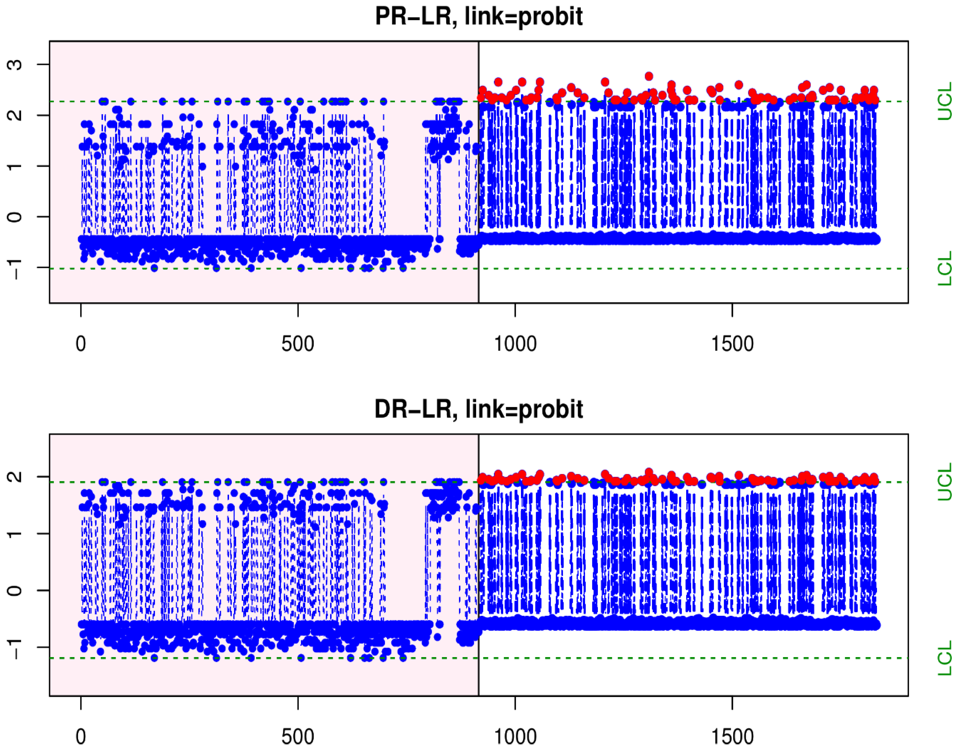
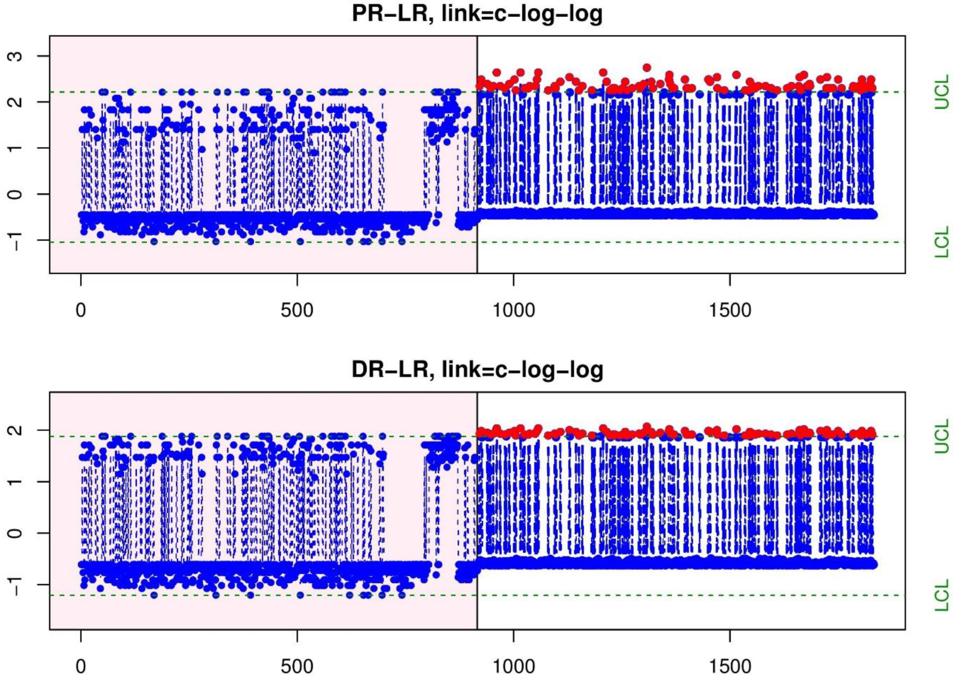
5. Application: COVID-19 Deaths Profile Monitoring

In this modern era, COVID-19 affects different people in different ways. Here, we monitor the mortality status of COVID-19 patients who were admitted to Benazir Bhutto Shaheed Hospital, Rawalpindi, Pakistan. This data had been already collected by Akhtar et al. [29], where they collected this data from three hospitals, and we are considering one of these hospital data sets. In this application, our response variable $\left(Y\right)$ is binary ($y=1$, if the COVID patient is discharged deceased; otherwise, $y=0$). Therefore, we consider this application for the evaluation of our proposed control charts. The data about the demographic and vital signs of all adult COVID-19 patients who were discharged from Benazir Bhutto Shaheed Hospital, Rawalpindi, during the first wave of COVID-19 (February to August 2020) were retrospectively collected. The National Early Warning Score (NEWS) was calculated by following the work of the Royal College of Physicians (RCP) (2012, page 14), and considered an independent variable in this study. The NEWS is based on a simple aggregate scoring system, which is computed based on vital signs (see

Table 5. The strategy to estimate national early warning score (NEWS).

Physiological Parameters	3	2	1	0	1	2	3
Respiration Rate	≤8		9–11	12–20		21–24	≥25
Oxygen Saturations	≤91	92–93	94–95	≥96
Any Supplemental Oxygen		Yes		No
Temperature	≤35.0		35.1–36.0	36.1–38.0	38.1–39.0	≥39.1
Systolic Blood Pressure	≤90	91–100	101–110	111–219			≥220
Heart Rate	≤40		41–50	51–90	91–110	111–130	≥131
Level of Consciousness				Alert			Voice, Pain, or Unconscious

[30]).

We had data of a total of 916 COVID-19 patients, consisting of mortality status $\left(y\right)$ and NEWS $\left(x\right)$. Based on the available data, we run logistic regression by setting logit, probit, c-log-log, and cauchit link functions. The Pearson (PR) and deviance (DR) residuals were obtained for estimated logistic regression models under each link function, and their means and standard deviations (SD) are reported in

Table 6. For the COVID-19 data, the mean and standard deviation of logistic regression residuals, control limits and OOC signals under different link functions.

Link Functions	logit		probit		c-log-log		cauchit
Residuals	PR	DR	PR	DR	PR	DR	PR	DR
Mean	−0.0019	−0.1476	−0.0011	−0.1468	−0.0015	−0.1473	−0.0078	−0.1529
SD	0.9971	1.0337	0.9979	1.034	0.9964	1.0345	0.9916	1.0352
LCL	−1.0234	−1.1939	−1.0152	−1.1873	−1.0375	−1.2051	−1.0591	−1.2222
UCL	2.256	1.899	2.277	1.9071	2.2192	1.8847	2.1154	1.8429
OOC Signals	83	97	83	83	97	97	144	144

. Further, we set $AR{L}_0=200$ and obtained the limits of PR and DR-based control charts, which are also given in Table 6. To make the OOC dataset, we have estimated a new response variable $\left(Y_1\right)$ by using ${\mu }_Y-uniform\left(0,0.2\right)$. Similarly, we estimated logistic regression models and obtained shifted PR’s and DR’s. The PR- and DR-based control charts under different link functions are presented in Figure 2, Figure 3, Figure 4 and Figure 5. The points under the pink and white shaded areas belong to the IC and OOC situation, respectively. The blue color points indicate the IC PR’s and DR’s, while the red color shows the OOC points. The PR- and DR-based control charts under the logit function are presented in Figure 2, while proposed control charts based on the probit function are portrayed in Figure 3. Figure 4 and Figure 5 consist of PR and DR-based control charts under c-log-log and cauchit link functions, respectively. The out-of-control points are counted for each chart and reported in Table 6. It is revealed that the PR- and DR-based control charts under the cauchit link function have captured a large number of OOC signals. The second largest OOC points were detected by the PR- and DR-based control charts for the c-log-log link function. Hence, PR- and DR-based control charts under cauchit link and c-log-log link functions outperform all their counterparts.

6. Conclusions

In this study, the control charts are constructed based on the LR residuals (Pearson residuals (PR) and deviance residuals (DR)) with different link functions (the logit, probit, c-log-log, and cauchit). We evaluate the performance of the control charts with the help of a simulation study, where ARL is considered as the evaluation criterion. The simulation study shows that in monitoring ${\beta }_0$, the c-log-log link function showed good performance for both PR and DR control charts as compared to the other link functions. While monitoring ${\beta }_1$, the DR-based control chart with the probit link function performs better as compared to the PR-based control charts and with other link functions due to its minimum ARL. We also conclude that in monitoring ${\mu }_x$, the logit link function gives a better performance for the DR-based control chart as compared to the PR-based control charts with other link functions. For the COVID-19 death data, the PR- and DR-based control charts were implemented and showed that charts based on the cauchit link function indicated a large number of signals. The 2nd link function which gives the 2nd largest OOC is the c-log-log link function. Therefore, it is concluded from the results that mostly the DR-based control charts with the c-log-log link function give a better performance as compared to the other link functions.

References

1. Mahmood, T.; Xie, M. Models and monitoring of zero-inflated processes: The past and current trends. Qual. Reliab. Eng. Int. 2019, 35, 2540–2557. [Google Scholar] [CrossRef]
2. Shewhart, W.A. Economic Control of Quality of Manufactured Product; Macmillan And Co., Ltd.: London, UK, 1931. [Google Scholar]
3. Page, E.S. Continuous inspection schemes. Biometrika 1954, 41, 100–115. [Google Scholar] [CrossRef]
4. Roberts, S.W. Control chart tests based on geometric moving averages. Technometrics 2000, 42, 97–101. [Google Scholar] [CrossRef]
5. Zhu, J.; Lin, D.K. Monitoring the slopes of linear profiles. Qual. Eng. 2009, 22, 1–12. [Google Scholar] [CrossRef]
6. Nelder, J.A.; Weddernburn, R.W.M. Generalized linear models. J. R. Stat. Soc. Ser. A 1972, 135, 370–384. [Google Scholar] [CrossRef]
7. Skinner, K.R.; Montgomery, D.C.; Runger, G.C. Process monitoring for multiple count data using generalized linear model-based control charts. Int. J. Prod. Res. 2003, 41, 1167–1180. [Google Scholar] [CrossRef]
8. Jearkpaporn, D.; Montgomery, D.C.; Runger, G.C.; Borror, C.M. Process monitoring for correlated gamma-distributed data using generalized-linear-model-based control charts. Qual. Reliab. Eng. Int. 2003, 19, 477–491. [Google Scholar] [CrossRef]
9. Skinner, K.R.; Montgomery, D.C.; Runger, G.C. Generalized linear model-based control charts for discrete semiconductor process data. Qual. Reliab. Eng. Int. 2004, 20, 777–786. [Google Scholar] [CrossRef]
10. Koosha, M.; Amiri, A. The effect of link function on the monitoring of logistic regression profiles. In Proceedings of the World Congress on Engineering 2011, London, UK, 6–8 July 2011. [Google Scholar]
11. Shu, L.; Tsui, K.L.; Tsung, F. Regression Control Charts. Encyclopedia of Statistics in Quality and Reliability. 2008. Available online: https://onlinelibrary.wiley.com/doi/abs/10.1002/9780470061572.eqr260 (accessed on 15 January 2023).
12. Asgari, A.; Amiri, A.; Niaki, S.T.A. A new link function in GLM-based control charts to improve monitoring of two-stage processes with Poisson response. Int. J. Adv. Manuf. Technol. 2014, 72, 1243–1256. [Google Scholar] [CrossRef]
13. Amiri, A.; Koosha, M.; Azhdari, A.; Wang, G. Phase I monitoring of generalized linear model-based regression profiles. J. Stat. Comput. Simul. 2015, 85, 2839–2859. [Google Scholar] [CrossRef]
14. Amiri, A.; Yeh, A.B.; Asgari, A. Monitoring two-stage processes with binomial data using generalized linear model-based control charts. Qual. Technol. Quant. Manag. 2016, 13, 241–262. [Google Scholar] [CrossRef]
15. Qi, D.; Wang, Z.; Zi, X.; Li, Z. Phase II monitoring of generalized linear profiles using weighted likelihood ratio charts. Comput. Ind. Eng. 2016, 94, 178–187. [Google Scholar] [CrossRef]
16. Moheghi, H.R.; Noorossana, R.; Ahmadi, O. GLM profile monitoring using robust estimators. Qual. Reliab. Eng. Int. 2021, 37, 664–680. [Google Scholar] [CrossRef]
17. Kinat, S.; Amin, M.; Mahmood, T. GLM-based control charts for the inverse Gaussian distributed response variable. Qual. Reliab. Eng. Int. 2020, 36, 765–783. [Google Scholar] [CrossRef]
18. García-Bustos, S.; Zambrano, G. Control charts for health surveillance based on residuals of negative binomial regression. Qual. Reliab. Eng. Int. 2022, 38, 2521–2532. [Google Scholar] [CrossRef]
19. Hakimi, A.; Amiri, A.; Kamranrad, R. Robust approaches for monitoring logistic regression profiles under outliers. Int. J. Qual. Reliab. Manag. 2017, 34, 494–507. [Google Scholar] [CrossRef]
20. Kim, J.-M.; Ha, I.D. Deep learning-based residual control chart for count data. Qual. Eng. 2022, 34, 370–381. [Google Scholar] [CrossRef]
21. Mahmood, T.; Iqbal, A.; Abbasi, S.A.; Amin, M. Efficient GLM-based control charts for Poisson processes. Qual. Reliab. Eng. Int. 2022, 38, 389–404. [Google Scholar] [CrossRef]
22. Soleimani, P.; Asadzadeh, S. Effect of non-normality on the monitoring of simple linear profiles in two-stage processes: A remedial measure for gamma-distributed responses. J. Appl. Stat. 2022, 49, 2870–2890. [Google Scholar] [CrossRef]
23. Yeganeh Chukhrova, N.; Johannssen, A.; Fotuhi, H. A network surveillance approach using machine learning based control charts. Expert Syst. Appl. 2023, 219, 119660. [Google Scholar] [CrossRef]
24. Yu, J.; Liu, J. LRProb control chart based on logistic regression for monitoring mean shifts of auto-correlated manufacturing processes. Int. J. Prod. Res. 2011, 49, 2301–2326. [Google Scholar] [CrossRef]
25. Khosravi, P.; Amiri, A. Self-Starting control charts for monitoring logistic regression profiles. Commun. Stat.-Simul. Comput. 2019, 48, 1860–1871. [Google Scholar] [CrossRef]
26. Alevizakos, V.; Koukouvinos, C.; Lappa, A. Comparative study of the Cp and Spmk indices for logistic regression profile using different link functions. Qual. Eng. 2019, 31, 453–462. [Google Scholar] [CrossRef]
27. Jahani, K.; Feili, H.; Ohadi, F. Phase II monitoring of the nominal logistic regression profiles based on Wald and Rao score test statistics (a case study in healthcare: Diabetic patients). Int. J. Product. Qual. Manag. 2019, 27, 161–176. [Google Scholar] [CrossRef]
28. Amin, M.; Mahmood, T.; Kinat, S. Memory type control charts with inverse-Gaussian response: An application to yarn manufacturing industry. Trans. Inst. Meas. Control 2021, 43, 656–678. [Google Scholar] [CrossRef]
29. Akhtar, H.; Akhtar, S.; Rahman, F.U.; Afridi, M.; Khalid, S.; Ali, S.; Akhtar, N.; Khader, Y.S.; Ahmad, H.; Khan, M.M. An overview of the treatment options used for the management of COVID-19 in Pakistan: Retrospective Observational Study. JMIR Public Health Surve. 2021, 7, e28594. [Google Scholar] [CrossRef]
30. Royal College of Physicians. National Early Warning Score (NEWS): Standardising the Assessment of Acute Illness Severity in the NHS; Report of a Working Party; RCP: London, UK, 2012. [Google Scholar]
Figure 1. Follow chart of the process.
Mathematics 11 01113 g001
Figure 2. Control chart based on PR and DR with the logit link function.
Mathematics 11 01113 g002
Figure 3. Control chart based on PR and DR with the probit link function.
Mathematics 11 01113 g003
Figure 4. Control chart based on PR and DR with the c-log-log link function.
Mathematics 11 01113 g004
Figure 5. Control chart based on PR and Dr with the cauchit link function.
Mathematics 11 01113 g005