Constrained Self-Adaptive Physics-Informed Neural Networks with ResNet Block-Enhanced Network Architecture

Abstract

Physics-informed neural networks (PINNs) have been widely adopted to solve partial differential equations (PDEs), which could be used to simulate physical systems. However, the accuracy of PINNs does not meet the needs of the industry, and severely degrades, especially when the PDE solution has sharp transitions. In this paper, we propose a ResNet block-enhanced network architecture to better capture the transition. Meanwhile, a constrained self-adaptive PINN (cSPINN) scheme is developed to move PINN’s objective to the areas of the physical domain, which are difficult to learn. To demonstrate the performance of our method, we present the results of numerical experiments on the Allen–Cahn equation, the Burgers equation, and the Helmholtz equation. We also show the results of solving the Poisson equation using cSPINNs on different geometries to show the strong geometric adaptivity of cSPINNs. Finally, we provide the performance of cSPINNs on a high-dimensional Poisson equation to further demonstrate the ability of our method.

1. Introduction

Deep learning achieves breakthroughs in many scientific fields and impacts the areas of data analysis, decision making, and pattern recognition. Recently, deep learning methods have been applied to solve partial differential equations (PDEs), and physics-informed neural networks (PINNs) [1,2] used to solve the partial differential equations (PDEs). The main idea is to represent the solutions of PDEs using a neural network, and optimize them with the constraints of physics-informed loss using automatic differentiation (AD). In the last few years, PINNs have been employed to solve PDEs from different fields, including problems in mechanical engineering, geophysics [3], vascular fluid dynamics [4,5], and biomedicine [6].

To further enhance the accuracy and efficiency of PINNs, a series of extensions to the original formulation of Raissi et al. [1,7,8,9,10,11] were proposed. For example, from the aspect of data augmentation, re-sampling methods are proposed to adaptively change the distribution of residual points during training [7,8], which could help to improve the accuracy of PINNs in solving stiff PDEs. The standard loss function in PINNs is the mean square error (MSE), which is not always suitable for training when solving PDEs [12,13]. In [9], an adjustment method among different loss terms was proposed to mitigate the gradient pathologies. Causal-PINNs [10] was proposed to solve the time-dependent PDEs, by means of an adaptive adjustment scheme for loss weights in the temporal domain. Meanwhile, regularization on the differential forms of PDEs was also demonstrated to be an effective way to improve accuracy [14], compared to original PINNs. In addition, the architectures [9,11,15,16] of PINNs greatly influence the final prediction results, and some works [15,17] have focused on embedding methods, which are useful for features enhancement of PINNs and are even possibly enforceable on soft/hard boundary enforcement [18].

PINNs with fully connected neural networks are widely used to solve partial differential equations and the derivatives of PDEs could be directly computed by means of automatic differentiation (AD). There also exist various types of architectures to solve PDEs, e.g., CNN architecture [19] and UNet architecture [20]. However, CNN and UNet require a finite difference approach when calculating the derivatives of PDEs. Other architectures, such as Bayesian neural networks (BNNs) [21] and generative adversarial networks(GANs) [22], are also used to address PDE problems. Despite the development of different architectures, fully connected feed forward neural networks are still the most used architecture in PINNs and their hyper-parameters, such as depth, width or the connected way between hidden layers, greatly influence the final results. In [16], adjustments on width and depth of fully connected neural networks (FCNNs) showed the different accuracy of PINNs. In [11], a ResNet-block was used to enhance the connected way between hidden layers and performed better than FCNNs in the parameters identification of the Navier–Stokes equation. As in [9], modified neural network was also proposed to project the input variables to a high-dimensional feature space and fuse them as neural attention mechanisms. All these cases showed that the selected architecture was essential to the final predictive results of PINNs.

The main idea of such an adaptive scheme is to attach a bounded trainable weight for each single residual point in the residual loss function and adaptively update pointwise weights for each training point. As for the architecture, it influences the predicted results and is also essential for improving the accuracy of PINN methods. Our contributions in this paper are summarized below:

• We develop a constrained self-adaptive physics-informed neural network (cSPINN), which had better accuracy in numerical results. Meanwhile, the dynamics of residual weights changed more steadily during the training process.
• To better capture the solution with sharp transitions in the physical domain, we develop a ResNet block-enhanced modified MLP architecture, which also has the ability to tackle the vanishing gradient problem using identity mapping, even for deep architectures.

2. Related Works

In this section, we first introduce the model problem, and then provide a brief overview of physics-informed neural networks (PINNs) for solving forward partial differential equations (PDEs).

2.1. Model Problem

In this subsection, we first introduce the model problem given the spatial domain $\mathsf{\Omega }$, and the temporal $t\in [0,T]$ domain, having the general form of a partial differential equation (PDE):

$$\begin{array}{cc}\hfill & {\mathcal{N}}_t\left[u(x,t)\right]+{\mathcal{N}}_x\left[u(x,t)\right]=0,x\in \mathsf{\Omega },t\in (0,T]\hfill \end{array}$$

(1a)

$$\begin{array}{cc}\hfill & u(x,0)=u_0\left(x\right),x\in \mathsf{\Omega }\hfill \end{array}$$

(1b)

$$\begin{array}{cc}\hfill & \mathcal{B}\left[u\right(x,t\left)\right]=g(x,t),x\in \partial \mathsf{\Omega },t\in (0,T]\hfill \end{array}$$

(1c)

where ${\mathcal{N}}_t[·]$ and ${\mathcal{N}}_x[·]$ are the general differential operator, which includes any combination of linear and non-linear terms of temporal and spatial derivatives. The corresponding initial condition at $t=0$ is given by $u_0\left(x\right)$. In the above, $\mathcal{B}[·]$ is a boundary operator, which could be Neumann, Robin, or periodic boundary conditions, and enforces the condition $g(x,t)$ at the boundary domain $\partial \mathsf{\Omega }$.

2.2. PINNs Formulation

To solve the PDEs via PINNs [1], we needed to construct a neural network $\widehat{u}(x,t;\mathit{w})$, given the spatial $x\in \mathsf{\Omega }$ and temporal $t\in [0,T]$ inputs with the trainable parameters $\mathit{w}$, to approximate the solution $u(x,t)$. Then, we could train a physics-informed model by minimizing the following loss function:

$$\begin{array}{c}\hfill \mathcal{L}\left(\mathit{w}\right)={\lambda }_r{\mathcal{L}}_r\left(\mathit{w}\right)+{\lambda }_{ic}{\mathcal{L}}_{ic}\left(\mathit{w}\right)+{\lambda }_{bc}{\mathcal{L}}_{bc}\left(\mathit{w}\right)\end{array}$$

(2)

where

$$\begin{array}{cc}\hfill & {\mathcal{L}}_r\left(\mathit{w}\right)=\frac{1}{N_r}\sum _{i=1}^{N_r}{\left|{\mathcal{N}}_t\left[u_{\mathit{w}}(x_r^i,t_r^i)\right]+{\mathcal{N}}_x\left[u_{\mathit{w}}(x_r^i,t_r^i)\right]\right|}^2,\hfill \end{array}$$

(3a)

$$\begin{array}{cc}\hfill & {\mathcal{L}}_{ic}\left(\mathit{w}\right)=\frac{1}{N_{ic}}\sum _{i=1}^{N_{ic}}{\left|u_{\mathit{w}}\left(x_{ic}^i,0\right)-u_0\left(x_{ic}^i\right)\right|}^2,\hfill \end{array}$$

(3b)

$$\begin{array}{cc}\hfill & {\mathcal{L}}_{bc}\left(\mathit{w}\right)=\frac{1}{N_{bc}}\sum _{i=1}^{N_{bc}}{\left|\mathcal{B}\left[u_{\mathit{w}}\right]\left(x_{bc}^i,t_{bc}^i\right)-g\left(x_{bc}^i,t_{bc}^i\right)\right|}^2\hfill \end{array}$$

(3c)

here, ${\mathcal{L}}_r$, ${\mathcal{L}}_{ic}$ and ${\mathcal{L}}_{bc}$ are loss functions due to the residual in physics domain, loss in initial condition and boundary condition. We use $u_{\mathit{w}}$ to represent the output of neural network, which is parameterized by $\mathit{w}$. ${\lambda }_r$, ${\lambda }_{ic}$ and ${\lambda }_{bc}$ are the weights that could influence the convergence rate of different loss components and the final accuracy of PINNs [9,12]. Hence, it was important to use an appropriate weighting strategy during training. Here ${\{x_r^i,t_r^i\}}_{i=1}^{N_r}$, ${\left\{x_{ic}^i\right\}}_{i=1}^{N_{ic}}$ and ${\{x_{bc}^i,t_{bc}^i\}}_{i=1}^{N_{bc}}$ are training points inside the domain, points on the initial domain and points on the boundary.

In this paper, we used $L^2$ error to define the relative error between the PINNs’ prediction and the reference solutions, as

$$\epsilon \left(x_k,t_k\right)=\frac{{\left[{\sum }_{k=1}^N{\left|\widehat{u}\left(x_k,t_k\right)-u\left(x_k,t_k\right)\right|}^2\right]}^{\frac{1}{2}}}{{\left[{\sum }_{k=1}^N{\left(u\left(x_k,t_k\right)\right)}^2\right]}^{1/2}}$$

where $u(x_k,t_k)$ is the reference solution and $\widehat{u}(x_k,t_k)$ is the neural network prediction for a set of testing points ${\left\{\left(x_k,t_k\right)\right\}}_{k=1}^N$ ($\left(x_k,t_k\right)\in \mathsf{\Omega }\times (0,T]$).

3. Formulation of Constrained Self-Adaptive PINNs (cSPINNs)

In this section, we first present the method of the constrained self-adaptive weighting scheme for PINNs, which could adaptively adjust the weights for residual points during training. Next, we propose a modified network architecture enhanced by ResNet block to further improve the performance of cSPINNs.

3.1. Constrained Self-Adaptive Weighting Scheme

In PINNs, we defined the residual loss ${\mathcal{L}}_r\left(\mathit{w}\right)$ to enforce the network to satisfy the governing equation for any sample points inside the domain, i.e., ${\{x_r^i,t_r^i\}}_{i=1}^{N_r}$. However, we could find that equal weight was attached for all residual points in the above formulation of ${\mathcal{L}}_r\left(\mathit{w}\right)$, with the result that PINNs could not focus on the area that was difficult to learn during training (as shown in Figure 1). One effective way to overcome this, was to attach individual adjustable weights for each residual point, according to the distribution of residual in the physical domain, and then automatically raise the weights of inner points with relatively higher loss value. Then, we could formulate such self-adaptive adjustment as a min–max optimization problem, i.e.,

$$\underset{\mathit{w}}{min}\underset{\widehat{{\lambda }_{\mathit{r}}}}{max}\mathcal{L}\left(\mathit{w},{\lambda }_r,{\lambda }_{ic},{\lambda }_{bc},\widehat{{\lambda }_{\mathbf{r}}}\right)$$

(4a)

$$\begin{array}{cc}\hfill s.t.& \sum _{i=1}^{N_r}{\widehat{{\lambda }_r}}_i=C\hfill \end{array}$$

(4b)

where $\widehat{{\lambda }_{\mathbf{r}}}:=\{{\widehat{{\lambda }_r}}_1,{\widehat{{\lambda }_r}}_2,\dots ,{\widehat{{\lambda }_r}}_{N_r}\}$ are trainable adaptive weights for all corresponding residual points ${\{x_r^i,t_r^i\}}_{i=1}^{N_r}$, and C is a constant that could be used to constrain the range of weights. Here, we set C as the expectation of weights in PINNs, i.e., $C=E\left({\sum }_{i=1}^{N_r}{\widehat{{\lambda }_r}}_i\right)=N_r$. The formulation of loss function is as below:

$$\mathcal{L}\left(\mathit{w},{\lambda }_r,{\lambda }_{ic},{\lambda }_{bc},\widehat{{\lambda }_{\mathbf{r}}}\right)={\lambda }_r{\mathcal{L}}_r(\mathit{w},\widehat{{\lambda }_{\mathbf{r}}})+{\lambda }_{ic}{\mathcal{L}}_{ic}\left(\mathit{w}\right)+{\lambda }_{bc}{\mathcal{L}}_{bc}\left(\mathit{w}\right)$$

where ${\mathcal{L}}_r(\mathit{w},\widehat{{\lambda }_{\mathbf{r}}})=\frac{1}{N_r}{\sum }_{i=1}^{N_r}{\widehat{{\lambda }_r}}_i{\left|{\mathcal{N}}_t\left[u_{\mathit{w}}(x_r^i,t_r^i)\right]+{\mathcal{N}}_x\left[u_{\mathit{w}}(x_r^i,t_r^i)\right]\right|}^2$ is a weighted residual loss and the other terms in $\mathcal{L}\left(\mathit{w},{\lambda }_r,{\lambda }_{ic},{\lambda }_{bc},\widehat{{\lambda }_{\mathbf{r}}}\right)$ are the same as in the original formulation. It was easy to solve the inner optimization of the min–max optimization problem above by selecting a residual point with the largest residual loss and attaching a weight with value C, while setting the weights of other points to zero.

Figure 1. PINNs results for solving Allen–Cahn Equation (The first row) and 2D Poisson’s Equation (The second row).

However, PINNs could only optimize one single point in every training iteration if we chose such a strategy, which went against the adjustment among different residual points. In [12], Mcclenny et al. proposed a self adaptive method to solve the above min–max problem by a step-forward optimization in the inner optimization using a gradient ascent procedure, which could approximately satisfy the inner maximization requirement. In this way, different residual points could be attached with appropriate weights during training. They updated the $\widehat{{\lambda }_{\mathbf{r}}}$ during the training process as:

$${\widehat{\lambda }}_r^{k+1}={\widehat{\lambda }}_r^k+{\eta }_k{\nabla }_{{\widehat{\lambda }}_r^k}\mathcal{L}\left(\mathit{w},{\lambda }_r,{\lambda }_{ic},{\lambda }_{bc},{\widehat{\lambda }}_r^k\right)$$

where ${\eta }_k$ is the learning rate at iteration k. However, it was easy to see that ${\widehat{\lambda }}_r^k$ was an unbounded weights vector during the training, which mean that the training of PINNs would suffer an unstable state, caused by the rapidly changing weights. We modified the updating rules of the ${\widehat{\lambda }}_r^k$ as:

$$\begin{array}{cc}\hfill {\lambda }_r^{k+1}& ={\widehat{\lambda }}_r^k+{\eta }_k{\nabla }_{{\widehat{\lambda }}_r^k}\mathcal{L}\left(\mathit{w},{\lambda }_r,{\lambda }_{ic},{\lambda }_{bc},{\widehat{\lambda }}_r^k\right)\hfill \end{array}$$

(5a)

$$\begin{array}{cc}\hfill {\lambda }_{r_i}^{k+1}& =\frac{|{\lambda }_{r_i}^{k+1}|}{{\sum }_{i=1}^{N_r}\left|{\lambda }_{r_i}^{k+1}\right|}\times C\hfill \end{array}$$

(5b)

$$\begin{array}{cc}\hfill {\widehat{\lambda }}_{r_i}^{k+1}& =(1-ϵ)\times {\widehat{\lambda }}_{r_i}^k+ϵ\times {\lambda }_{r_i}^{k+1},\hfill \end{array}$$

(5c)

where we denote $r_i$ as ith residual points in ${\{x_r^i,t_r^i\}}_{i=1}^{N_r}$, k and $k+1$ the training iteration numbers. ${\lambda }_r^{k+1}$ is a middle variable before normalization. In other words, we first normalized the ${\lambda }_{r_i}^{k+1}\in {\lambda }_r^{k+1}$ and derived the final ${\widehat{\lambda }}_{r_i}^{k+1}$ by a weighted sum of the previous weight ${\widehat{\lambda }}_{r_i}^k$ of iteration k and the normalized ${\lambda }_{r_i}^{k+1}$ in the current $k+1$ iteration. The framework of cSPINN is shown in Figure 2.

Figure 2. A framework of constrained self-adaptive physics-informed neural networks. A neural network output the solution u for PDE, then we computed the derivatives by auto differentiation and obtained the loss of initial conditions, boundary conditions and governing equation. The parameters of neural network and constrained self-adaptive weights for residual points were updated at the same time by means of the gradient method.

3.2. ResNet Block-Enhanced Modified Network

Continuous improvement of network structure design is one of the drivers for the development of deep learning methods and its applications. For example, convolutional neural networks [23,24,25] were designed for, and have been widely used in, computer vision, such as image classification, image segmentation, and object recognition tasks. Similarly, recurrent neural networks and their variants [26,27,28] show great performance in natural language processing and sequential modeling because of their ability to capture long-term dependencies in the sequences. In [9], a modified MLP framework was proposed to correctly capture the solution of complex PDEs, which has been widely used in many cases. PINNs with ResNet blocks are also used to improve the representational capacity of the neural network when solving PDEs. Inspired by these ideas, we proposed a ResNet block-enhanced modified MLP framework to better represent the solution of PDEs. The ResNet block-enhanced modified network is as follows:

$$\begin{array}{cc}\hfill & U=\varphi \left(X{W}^1+b^1\right),V=\varphi \left(X{W}^2+b^2\right)\hfill \end{array}$$

(6a)

$$\begin{array}{cc}\hfill & H^{\left(1\right)}=\varphi \left(X{W}^{z,1}+b^{z,1}\right)\hfill \end{array}$$

(6b)

$$\begin{array}{cc}\hfill & Z^{\left(k\right)}=\frac{1}{2}(H^{\left(k\right)}+F\left(H^{\left(k\right)}\right)),k=1,\dots ,L\hfill \end{array}$$

(6c)

$$\begin{array}{cc}& H^{(k+1)}=\left(1-Z^{\left(k\right)}\right)\odot U+Z^{\left(k\right)}\odot V,k=1,\dots ,L\hfill \end{array}$$

(6d)

$$\begin{array}{cc}\hfill & f=H^{(L+1)}W+b\hfill \end{array}$$

(6e)

here $\varphi$ is an activation function, ⊙ is an element-wise multiplication operation, f is the final output of network and the updating rule of $Z^{\left(k\right)}$ is similar to the residual learning, which was first proposed in [23] and achieved great success. We have denoted it above, i.e.,

$$\begin{array}{c}\hfill Z^{\left(k\right)}=\frac{1}{2}(H^{\left(k\right)}+F\left(H^{\left(k\right)}\right)),k=1,\dots ,L\end{array}$$

(7)

More specifically, $H^{\left(k\right)}$ and $Z^{\left(k\right)}$ are the input and output of the ResNet block, respectively. F is an operation consisting of a fully connected layer and activation function, which could be defined as $F\left(X\right):=\varphi (\varphi (X{W}^{1,k}+b^{1,k})W^{2,k}+b^{2,k})$ here, with input X, hidden layers’ parameters $\{W^{1,k},b^{1,k},W^{2,k},b^{2,k}\}$ and an activation function $\varphi$. As for the element-wise addition $H^{\left(k\right)}+F\left(H^{\left(k\right)}\right)$, it could be conducted by a shortcut connection. The effectiveness of such a block in PINNs was demonstrated in [11] and here we used it as a feature enhanced sub-structure of our network. The features could be fused by a shortcut connection and fed into updating the hidden layers by an element-wise multiplication operation with U and V, as shown in Figure 3. Compared to simple fully connected neural networks, our architecture enhanced the representative ability of hidden layers by ResNet blocks, which could make it easier for the network to learn the desired solution. Meanwhile, embedding of inputs from low-level space to higher dimensional feature space could also be considered here, and could be fused, using the attention mechanism during the forward process.

Figure 3. The ResNet block-enhanced modified architecture for physics-informed neural networks.

4. Numerical Experiments

We demonstrated the performance of our proposed cSPINN in solving several PDE problems. In all of the examples, we used the ResNet block-enhanced modified network with tanh function as our activation function $\varphi$. The proposed architecture had 2 input neurons and consisted of 4 ResNet blocks, each having a width of 64. The output layer contained only one neuron for the output/solution of the PDE.

4.1. 1D Allen–Cahn Equation

The Allen–Cahn equation is a stiff PDE, which has a sharp interface and time transitions in its solution. We denote the 1D Allen–Cahn equation as below:

$$\begin{array}{cc}\hfill & u_t-0.0001u_{xx}+5u^3-5u=0,t\in [0,1],x\in [-1,1]\hfill \end{array}$$

(8a)

$$\begin{array}{cc}\hfill & u(x,0)=x^{2}cos\left(\pi x\right),\hfill \end{array}$$

(8b)

$$\begin{array}{cc}\hfill & u(-1,t)=u(1,t),\hfill \end{array}$$

(8c)

$$\begin{array}{cc}\hfill & u_x(-1,t)=u_x(1,t)\hfill \end{array}$$

(8d)

We used the same physics parameters of the Allen–Cahn equation as in [7] to better compare the results. For the given problem, we used the ResNet block-enhanced modified network architecture mentioned above to better fit the sharp transition. In order to implement the cSPINNs for the Allen–Cahn equation, the following loss function was used:

• The constrained self adaptive loss for the residual of the governing equation

  $$\begin{array}{cc}\hfill & R:={\widehat{u}}_t-0.0001{\widehat{u}}_{xx}+5{\widehat{u}}^3-5\widehat{u},\left(x_r^i,t_r^i\right)\in \mathsf{\Omega }\hfill \end{array}$$

  (9a)

  $$\begin{array}{cc}\hfill & MS{E}_R=\frac{1}{N_r}\sum _{i=1}^{N_r}{\widehat{\lambda }}_{r_i}{\left(R\left(x_r^i,t_r^i\right)\right)}^2\hfill \end{array}$$

  (9b)
• Mean squared loss on the initial condition

  $$\begin{array}{cc}\hfill & I:=\widehat{u}\left(x_{ic}^i,0\right)-{\left(x_{ic}^i\right)}^{2}cos\left(\pi x_{ic}^i\right),x_{ic}^i\in \Gamma \hfill \end{array}$$

  (10a)

  $$\begin{array}{cc}\hfill & MS{E}_I=\frac{1}{N_{ic}}\sum _{i=1}^{N_{ic}}{\left(I\left(x_{ic}^i,t_{ic}^i\right)\right)}^2\hfill \end{array}$$

  (10b)
• Mean squared loss on the boundary condition

  $$\begin{array}{cc}\hfill & B_1:=\widehat{u}(-1,t_b^i)-\widehat{u}(1,t_b^i),\hfill \end{array}$$

  (11a)

  $$\begin{array}{cc}\hfill & B_2:={\widehat{u}}_x(-1,t_b^i)-{\widehat{u}}_x(1,t_b^i),t_b^i\in \partial \mathsf{\Omega }\hfill \end{array}$$

  (11b)

  $$\begin{array}{cc}\hfill & MS{E}_B=\frac{1}{N_b}\sum _{i=1}^{N_b}{\left(B_1\left(x_b^i,t_b^i\right)\right)}^2+{\left(B_2\left(x_b^i,t_b^i\right)\right)}^2\hfill \end{array}$$

  (11c)

  where $\widehat{u}$ is the prediction of neural network and we sampled $N_r$ = 25,600 residual points, $N_b=400$ boundary points and $N_{ic}=512$ points on the initial condition. Here, we used the Adam optimizer with 10,000 epochs and L-BFGS optimizer with 1000 epochs to optimize the network architecture. During the training process, we set the boundary weight and the initial weight $w_b=w_i=100$, which could help expedite the convergence. Figure 4 shows the numerical results of constrained self-adaptive PINNs(cSPINNs) compared with the reference solution obtained through the Chebfun method [29] and the training loss history. The relative $L^2$ error was 1.472 × 10${}^{-2}$, which was better than the time-adaptive approach in [7] and the original PINNs [1].
  

  Figure 4. cSPINNs results (with ResNet block-enhanced) for solving 1D Allen–Cahn equation.

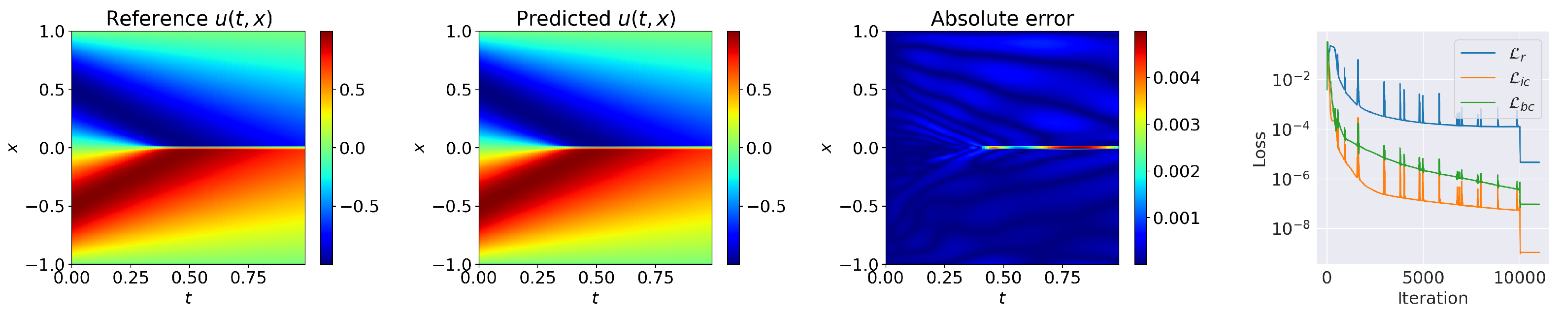
4.2. 1D Viscous Burgers’ Equation

The Viscous Burgers’ equation is widely used in various areas of applied mathematics, such as fluid mechanics, traffic flow, and gas dynamics. The 1D viscous Burgers equation could be denoted as below:

$$\begin{array}{cc}\hfill & u_t+u{u}_x-(0.01/\pi )u_{xx}=0,t\in [0,1],x\in [-1,1]\hfill \end{array}$$

(12a)

$$\begin{array}{cc}\hfill & u(0,x)=-sin\left(\pi x\right),\hfill \end{array}$$

(12b)

$$\begin{array}{cc}\hfill & u(t,-1)=u(t,1)=0\hfill \end{array}$$

(12c)

To better compare the results, we used the same physics parameters of the Burgers equation as in [1]. In order to implement the cSPINN scheme for the Burgers equation, the following modified residual loss function was used as mentioned in the formulation of cSPINNs:

• The constrained self adaptive loss for the residual of the governing equation

  $$\begin{array}{cc}\hfill & R:={\widehat{u}}_t+\widehat{u}{\widehat{u}}_x-(0.01/\pi ){\widehat{u}}_{xx},\left(x_r^i,t_r^i\right)\in \mathsf{\Omega }\hfill \end{array}$$

  (13a)

  $$\begin{array}{cc}\hfill & MS{E}_R=\frac{1}{N_r}\sum _{i=1}^{N_r}{\widehat{\lambda }}_{r_i}{\left(R\left(x_r^i,t_r^i\right)\right)}^2\hfill \end{array}$$

  (13b)
• Mean squared loss on the initial condition

  $$\begin{array}{cc}\hfill & I:=\widehat{u}\left(x_{ic}^i,0\right)+sin\left(\pi x_{ic}^i\right),x_{ic}^i\in \Gamma \hfill \end{array}$$

  (14a)

  $$\begin{array}{cc}\hfill & MS{E}_I=\frac{1}{N_{ic}}\sum _{i=1}^{N_{ic}}{\left(I\left(x_{ic}^i,t_{ic}^i\right)\right)}^2\hfill \end{array}$$

  (14b)
• Mean squared loss on the boundary conditions

  $$\begin{array}{cc}\hfill & B_1:=\widehat{u}(-1,t_b^i)-0,\hfill \end{array}$$

  (15a)

  $$\begin{array}{cc}\hfill & B_2:=\widehat{u}(1,t_b^i)-0,t_b^i\in \partial \mathsf{\Omega }\hfill \end{array}$$

  (15b)

  $$\begin{array}{cc}\hfill & MS{E}_B=\frac{1}{N_b}\sum _{i=1}^{N_b}{\left(B_1\left(-1,t_b^i\right)\right)}^2+{\left(B_2\left(1,t_b^i\right)\right)}^2\hfill \end{array}$$

  (15c)
  Here, we trained the network with a constrained self-adaptive scheme and $\widehat{u}$ was the prediction of neural network. In this case, we sampled $N_r$ = 25,600 residual points, $N_b=256$ boundary points and $N_{ic}=512$ points on the initial condition. We set the weights of initial condition and boundary condition as $N_{ic}=N_{bc}=100$. Training was performed using 10,000 Adam iterations and 1000 L-BFGS epochs. The predicted solution of cSPINNs, and loss history are shown in Figure 5. Despite a sharp transition in the center of the domain, the solution of cSPINNs was still accurate in the whole domain, yielding a relative $L^2$ error of 4.796 × 10${}^{-4}$.
  

  Figure 5. cSPINNs results (with ResNet block-enhanced modified neural network) for solving 1D viscous Burgers equation.

4.3. 2D Helmholtz Equation

The Helmholtz equation is widely used to describe the behavior of wave propagation, which could be mathematically formulated as follows:

$$\begin{array}{cc}\hfill & \mathsf{\Delta }u(x,y)+k^{2}u(x,y)-q(x,y)=0\hfill \end{array}$$

(16a)

$$\begin{array}{cc}\hfill & u(-1,y)=u(1,y)=u(x,-1)=u(x,1)=0\hfill \end{array}$$

(16b)

where $x\in [-1,1],y\in [-1,1]$ and

$$\begin{array}{cc}\hfill q(x,y)=& -{\left(a_1\pi \right)}^{2}sin\left(a_1\pi x\right)sin\left(a_2\pi y\right)-{\left(a_2\pi \right)}^{2}sin\left(a_1\pi x\right)sin\left(a_2\pi y\right)\hfill \\ \hfill & +k^{2}sin\left(a_1\pi x\right)sin\left(a_2\pi y\right)\hfill \end{array}$$

(17)

is a forcing term that results in a closed-form analytical solution

$$\begin{array}{cc}\hfill & u(x,y)=sin\left(a_1\pi x\right)sin\left(a_2\pi y\right)\hfill \end{array}$$

(18)

The exact solution above was as the same as in [9], which helped us better compare the results.

• The constrained self adaptive loss for the residual of the governing equation

  $$\begin{array}{cc}\hfill & R:=\mathsf{\Delta }\widehat{u}(x_r^i,y_r^i)+k^2\widehat{u}(x_r^i,y_r^i)-q(x_r^i,y_r^i),\left(x_r^i,y_r^i\right)\in \mathsf{\Omega }\hfill \end{array}$$

  (19a)

  $$\begin{array}{cc}\hfill & MS{E}_R=\frac{1}{N_r}\sum _{i=1}^{N_r}{\widehat{\lambda }}_{r_i}{\left(R\left(x_r^i,t_r^i\right)\right)}^2\hfill \end{array}$$

  (19b)
• Mean squared loss on the boundary conditions

  $$\begin{array}{cc}\hfill & B_1:=\widehat{u}(-1,y_b^i)-0,\hfill \end{array}$$

  (20a)

  $$\begin{array}{cc}\hfill & B_2:=\widehat{u}(1,y_b^i)-0,\hfill \end{array}$$

  (20b)

  $$\begin{array}{cc}\hfill & B_3:=\widehat{u}(x_b^i,-1)-0,\hfill \end{array}$$

  (20c)

  $$\begin{array}{cc}\hfill & B_4:=\widehat{u}(x_b^i,1)-0,\hfill \end{array}$$

  (20d)

  $$\begin{array}{cc}\hfill & MS{E}_B=\frac{1}{N_b}\sum _{i=1}^{N_b}{\left(B_1\left(-1,y_b^i\right)\right)}^2+{\left(B_2\left(1,y_b^i\right)\right)}^2+{\left(B_3\left(x_b^i,-1\right)\right)}^2+{\left(B_4\left(x_b^i,1\right)\right)}^2\hfill \end{array}$$

  (20e)

Here, we solved the problem with $a_1=1$ and $a_2=4$ to allow a direct comparison with the results reported in [9]. In this case, the ResNet block-enhanced modified network was trained with 10,000 Adam and 1000 L-BFGS epochs. As for the training points, we sampled $N_r$ = 10,000 residual points and $N_b=400$ (100 points per boundary). We show the prediction results of the cSPINNs in Figure 6. Finally, we achieved a relative $L^2$ error of 1.626 × 10${}^{-3}$, which exhibited performance than the learning-rate annealing weighted scheme, proposed in [9], and self-adaptive PINNs, proposed in [12]. Meanwhile, our method required less computational cost, due to the stability of the design in the self-adaptive weights.

Figure 6. cSPINNs results (with ResNet block-enhanced modified neural network) for solving the 2D Helmholtz equation with an exact solution.

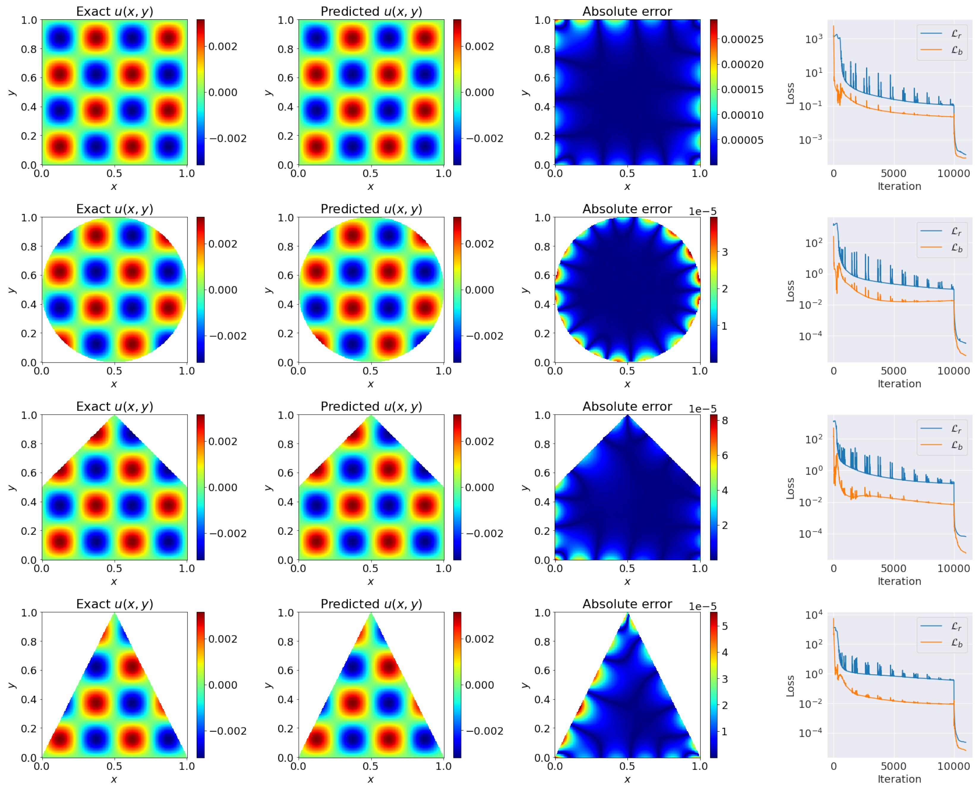
4.4. 2D Poisson Equation on Different Geometries

Poisson’s equation is an elliptic partial differential equation widely used in the description of potential fields. The 2D Poisson’s problem could be denoted as follows:

$$\begin{array}{cc}\hfill -\mathsf{\Delta }u& =f(x,y),(x,y)\in \mathsf{\Omega }\hfill \end{array}$$

(21)

$$\begin{array}{cc}\hfill u& =g(x,y),(x,y)\in \partial \mathsf{\Omega }\hfill \end{array}$$

(22)

To further demonstrate the performance of cSPINNs, we used the exact solution with periodicity $u(x,y)=\frac{1}{2{\left(4\pi \right)}^2}sin\left(4\pi x\right)sin\left(4\pi y\right)$ and obtained $f(x,y)$ and $g(x,y)$, according to the exact solution, directly as:

$$\begin{array}{cc}\hfill \mathsf{\Delta }u& =-sin\left(4\pi x\right)sin\left(4\pi y\right),(x,y)\in \mathsf{\Omega }\hfill \end{array}$$

(23)

$$\begin{array}{cc}\hfill u& =\frac{1}{2{\left(4\pi \right)}^2}sin\left(4\pi x\right)sin\left(4\pi y\right),(x,y)\in \partial \mathsf{\Omega }\hfill \end{array}$$

(24)

Then, we had the following loss terms

• The constrained self adaptive loss for the residual of the governing equation:

  $$\begin{array}{cc}\hfill & R:=-\mathsf{\Delta }\widehat{u}(x_r^i,y_r^i)+sin\left(4\pi x_r^i)sin(4\pi y_r^i\right),\left(x_r^i,y_r^i\right)\in \mathsf{\Omega }\hfill \end{array}$$

  (25a)

  $$\begin{array}{cc}\hfill & MS{E}_R=\frac{1}{N_r}\sum _{i=1}^{N_r}{\widehat{\lambda }}_{r_i}{\left(R\left(x_r^i,y_r^i\right)\right)}^2\hfill \end{array}$$

  (25b)
• Mean squared loss on the boundary conditions (Taking the rectangular area as example):

  $$\begin{array}{cc}\hfill & B_1:=\widehat{u}(-\frac{1}{4},y_b^i)-\frac{1}{2{(4\pi )}^2}sin(4\pi \times (-\frac{1}{4}))sin(4\pi y_b^i),y_b^i\in \partial {\mathsf{\Omega }}_l\hfill \end{array}$$

  (26a)

  $$\begin{array}{cc}\hfill & B_2:=\widehat{u}(\frac{1}{4},y_b^i)-\frac{1}{2{(4\pi )}^2}sin(4\pi \times \frac{1}{4})sin(4\pi y_b^i),y_b^i\in \partial {\mathsf{\Omega }}_r,\hfill \end{array}$$

  (26b)

  $$\begin{array}{cc}\hfill & B_3:=\widehat{u}(x_b^i,-\frac{1}{4})-\frac{1}{2{(4\pi )}^2}sin(4\pi x_b^i)sin(4\pi \times (-\frac{1}{4})),x_b^i\in \partial {\mathsf{\Omega }}_w,\hfill \end{array}$$

  (26c)

  $$\begin{array}{cc}\hfill & B_4:=\widehat{u}(x_b^i,\frac{1}{4})-\frac{1}{2{(4\pi )}^2}sin(4\pi x_b^i)sin(4\pi \times \frac{1}{4}),x_b^i\in \partial {\mathsf{\Omega }}_u,\hfill \end{array}$$

  (26d)

  $$\begin{array}{cc}\hfill & MS{E}_B=\frac{1}{N_b}\sum _{i=1}^{N_b}{\left(B_1\left(-\frac{1}{4},y_b^i\right)\right)}^2+{\left(B_2\left(\frac{1}{4},y_b^i\right)\right)}^2+{\left(B_3\left(x_b^i,-\frac{1}{4}\right)\right)}^2+{\left(B_4\left(x_b^i,\frac{1}{4}\right)\right)}^2\hfill \end{array}$$

  (26e)

In this case, we first tested the performance of cSPINNs on a rectangular domain ${\mathsf{\Omega }}_1=[0,0.25]\times [0,0.25]$. We sampled $N_r$ = 10,000 residual points in the inner domain and $N_b$ = 1000 boundary points distributed on the boundary area. The ResNet block-enhanced modified network was trained with 10,000 epochs Adam and 1000 epochs L-BFGS. Meanwhile, different geometries, including circular, triangular, and pentagonal domains, were also tested to demonstrate the advantages of cSPINNs. The $L^2$ error between the predicted solution and the reference solution on different geometries is shown in Table 1. It is worth noting that we magnified the loss value by a constant number of c = 10,000, due to the relatively small true value (the maximum value of exact solution was about 0.003) in the solution, to ensure normal gradient backward during training. As for an irregular domain, we sampled the same number of points as for the rectangular domain. We found that the cSPINNs achieved good performance in this problem, as shown in Figure 7. The original PINNs failed, as shown in Figure 1.

Table 1. The 2D Poisson equation: Relative $L^2$ errors obtained by cSPINN on different geometries. (${\mathsf{\Omega }}_1=[0,0.25]\times [0,0.25]$).

The 2D Poisson Equation	Relative ${\mathit{L}}^2$ Error (Inner)	Relative ${\mathit{L}}^2$ Error (Boundary)
Rectangular area	4.844 × 10${}^{-4}$	NaN
Circular area	4.349 × 10${}^{-4}$	2.258 × 10${}^{-3}$
Triangle area	3.375 × 10${}^{-4}$	8.735 × 10${}^{-4}$
Pentagon area	4.304 × 10${}^{-4}$	1.527 × 10${}^{-3}$

Figure 7. cSPINNs results (with ResNet block-enhanced modified neural network) for solving the 2D Poisson equation with an exact solution $u(x,y)=\frac{1}{2{\left(4\pi \right)}^2}sin\left(4\pi x\right)sin\left(4\pi y\right)$ in ${\mathsf{\Omega }}_1=[0,0.25]\times [0,0.25]$.

Moreover, we provided the comparison results between cSPINNs and reference solutions in the domain ${\mathsf{\Omega }}_2=[0,1]\times [0,1]$, which was hard for PINNs to solve, due to the high frequency of the solution, as shown in Figure 8. We show the relative $L^2$ errors between the predicted and the exact solution $u(x,y)$ using cSPINNs on the different geometries in Table 2. To further test the performance of cSPINNs, we provided the numerical results of cSPINNs on the L-shaped domain, a classic concave geometry. In this case, we set $f(x,y)=1$ and $g(x,y)=0$ to have a direct comparison with PINN, as in [30]. We had the loss terms as follow:

Figure 8. cSPINNs results (with ResNet block-enhanced modified neural network) for solving the 2D Poisson equation with an exact solution $u(x,y)=\frac{1}{2{\left(4\pi \right)}^2}sin\left(4\pi x\right)sin\left(4\pi y\right)$ in ${\mathsf{\Omega }}_2=[0,1]\times [0,1]$.

Table 2. The 2D Poisson equation: Relative $L^2$ errors obtained by cSPINN on different geometries. (${\mathsf{\Omega }}_2=[0,1]\times [0,1]$).

The 2D Poisson Equation	Relative ${\mathit{L}}^2$ Error (Inner)	Relative ${\mathit{L}}^2$ Error (Boundary)
Rectangular	2.522 × 10${}^{-3}$	NaN
Circular	1.748 × 10${}^{-3}$	1.077 × 10${}^{-2}$
Triangular	4.154 × 10${}^{-3}$	1.418 × 10${}^{-2}$
Pentagonal	2.329 × 10${}^{-3}$	6.309 × 10${}^{-3}$

• The constrained self adaptive loss for the residual of the governing equation

  $$\begin{array}{cc}\hfill & R:=-\mathsf{\Delta }\widehat{u}(x_r^i,y_r^i)-1,\left(x_r^i,y_r^i\right)\in \mathsf{\Omega }\hfill \end{array}$$

  (27a)

  $$\begin{array}{cc}\hfill & MS{E}_R=\frac{1}{N_r}\sum _{i=1}^{N_r}{\widehat{\lambda }}_{r_i}{\left(R\left(x_r^i,y_r^i\right)\right)}^2\hfill \end{array}$$

  (27b)
• Mean squared loss on the boundary condition

  $$\begin{array}{cc}\hfill & B:=\widehat{u}(x_b^i,y_b^i)-0,(x_b^i,y_b^i)\in \partial \mathsf{\Omega }\hfill \end{array}$$

  (28a)

  $$\begin{array}{cc}\hfill & MS{E}_B=\frac{1}{N_b}\sum _{i=1}^{N_b}{\left(B\left(x_b^i,y_b^i\right)\right)}^2\hfill \end{array}$$

  (28b)

We tested the performance of cSPINN on the L-shaped domain and show the results in Figure 9. The maximum point-wise error was yielded at about 6 × 10${}^{-3}$ and the relative $L^2$ error 4.257 × 10${}^{-3}$. In [30], PINNs achieved accurate results with about 0.02 maximum point-wise error in the same case on the L-shaped domain. In [31], hp-VPINNs also tested the performance and, in this case, achieved about 0.02 maximum point-wise error on the domain. Therefore, cSPINNs also performed well, even on such concave geometry.

Figure 9. cSPINNs results (with ResNet block-enhanced modified neural network) for solving the L-shaped Poisson equation with the reference solution.

4.5. High Dimensional Poisson Equation

Consider Poisson’s equation in high dimension (d = 10):

$$\begin{array}{cc}\hfill -\mathsf{\Delta }u=0,& x\in {(0,1)}^{10}\hfill \end{array}$$

(29)

$$\begin{array}{cc}\hfill u\left(x\right)=\sum _{k=1}^5{x}_{2k-1}{x}_{2k},& x\in \partial {(0,1)}^{10}\hfill \end{array}$$

(30)

The solution of this problem was $u\left(x\right)={\sum }_{k=1}^5{x}_{2k-1}{x}_{2k}$ and we computed the error of cSPINN using this exact solution.

• The constrained self adaptive loss for the residual of the governing equation:

  $$\begin{array}{cc}\hfill & R:=-\mathsf{\Delta }\widehat{u}({x_1}_r^i,{x_2}_r^i,\dots ,{x_{10}}_r^i),\left({x_1}_r^i,{x_2}_r^i,\dots ,{x_{10}}_r^i\right)\in \mathsf{\Omega }\hfill \end{array}$$

  (31a)

  $$\begin{array}{cc}\hfill & MS{E}_R=\frac{1}{N_r}\sum _{i=1}^{N_r}{\widehat{\lambda }}_{r_i}{\left(R\left(x_r^i,y_r^i\right)\right)}^2\hfill \end{array}$$

  (31b)
• Mean squared loss on the boundary condition:

  $$\begin{array}{cc}\hfill & B:=\widehat{u}({x_1}_b^i,{x_2}_b^i,\dots ,{x_{10}}_b^i)-\sum _{k=1}^5{x}_{2k-1}{x}_{2k},({x_1}_b^i,{x_2}_b^i,\dots ,{x_{10}}_b^i)\in \partial \mathsf{\Omega }\hfill \end{array}$$

  (32a)

  $$\begin{array}{cc}\hfill & MS{E}_B=\frac{1}{N_b}\sum _{i=1}^{N_b}{\left(B({x_1}_b^i,{x_2}_b^i,\dots ,{x_{10}}_b^i)\right)}^2\hfill \end{array}$$

  (32b)

We computed the relative $L^2$ error between the solution of cSPINN and the exact solution. The relative $L^2$ error of cSPINN was 1.028 × 10${}^{-3}$, which was smaller than the Deep Ritz method [32] (about 0.4%). In this case, we sampled $N_r$ = 1000 residual points in the inner domain and $N_b$ = 100 boundary points distributed on the boundary area. The ResNet block-enhanced modified network was trained with 20,000 epochs Adam and 1000 epochs L-BFGS. The training loss history of cSPINN is shown in Figure 10. Finally, we also provide the relative computational cost between cSPINNs and PINNs in different cases in Table 3. When computing the cost, we set the cSPINNs and PINNs with the same network depth, width, and number of training epochs for fair comparison.

Figure 10. cSPINNs’ training loss for High Dimensional Poisson equation. (with ResNet block-enhanced modified neural network).

Table 3. The relative computational cost of solving different PDEs with cSPINNs and PINNs.

Equation	PINNs	cSPINNs
1D Allen-Cahn	1.000	2.123
1D Burgers	1.000	2.346
2D Helmholtz	1.000	2.121
2D Poisson	1.000	2.101
HD Poisson	1.000	2.709

At the end of this section, we also tested the impact of the following three architectures: the Multilayer Perceptron(MLP), the modified Multilayer Perceptron (MMLP), and the ResNet block-enhanced modified network(ResMNet). During the test, the depth and width of all networks were fixed at 6 and 128, respectively. Here, we also provided the results to demonstrate the effectiveness of our proposed constrained self-adaptive weighting scheme(cSA) compared to the $L^2$ loss function. Meanwhile, as can be seen in Table 4, we observed that, compared to the MLP and the MMLP, the ResMNet yielded the highest accuracy. Therefore, the constrained self-adaptive weighting scheme (cSA) and the ResNet block-enhanced modified network (ResMNet) were desired in the cSPINNs.

Table 4. Relative $L^2$ errors of different loss functions and different architectures.

Equation	L2 loss+MLP	L2 loss+ResMNet	cSA+MMLP	cSA+ResMNet
1D Allen-Cahn	9.63 × 10${}^{-1}$	2.38 × 10${}^{-2}$	1.61 × 10${}^{-2}$	1.16 × 10${}^{-2}$
1D Burgers	6.70 × 10${}^{-4}$	4.68 × 10${}^{-4}$	3.80 × 10${}^{-4}$	2.70 × 10${}^{-4}$
2D Helmholtz	4.69 × 10${}^{-3}$	3.61 × 10${}^{-3}$	1.01 × 10${}^{-3}$	9.50 × 10${}^{-4}$
2D Poisson (Rectangular)	3.58 × 10${}^{-2}$	1.64 × 10${}^{-2}$	1.12 × 10${}^{-2}$	1.94 × 10${}^{-3}$
2D Poisson (L-shaped)	5.65 × 10${}^{-3}$	4.82 × 10${}^{-3}$	4.26 × 10${}^{-3}$	3.78 × 10${}^{-3}$
HD Poisson (d = 10)	1.33 × 10${}^{-3}$	1.01 × 10${}^{-3}$	1.25 × 10${}^{-3}$	8.62 × 10${}^{-4}$

5. Conclusions and Future

In this paper, we proposed constrained self-adaptive PINNs (cSPINNs) to adaptively adjust the weights of individual residual points, which became more robust during training, due to the bounded weights. Meanwhile, a ResNet block-enhanced modified neural network was also proposed to enhance the predictive ability of PINNs.

We demonstrated the effectiveness of our method in solving various PDEs, including the Allen–Cahn equation, the Burgers equation, the Poisson equation and the Helmholtz equation. Our method showed good performance in all the cases mentioned and outperformed PINNs, especially in the Poisson equation with periodic solution, regardless of the geometries of the computational domain. Even with sharp transition in the physical domain, cSPINNs were also robust when solving the Allen–Cahn equation, which was difficult for the original PINNs to solve. Compared with the PINNs, cSPINNs could improve the accuracy and could be implemented with just a few lines of code, which made it possible to combine our method with other extensions of PINNs to further improve the performance.

The usage of a constrained self-adaptive weighting scheme could attach higher weight values to difficult to learn regions during training, which made it possible to solve complicated problems. In this paper, we provided the numerical results of cSPINNs in solving the 10D Poisson equation and achieved better performance than the Deep-Ritz method. In the future, we will further generalize cSPINNs to solve higher dimensional PDEs and multi-physics problems.

References

- Raissi, M.; Perdikaris, P.; Karniadakis, G. Physics-informed neural networks: A deep learning framework for solving forward and inverse problems involving nonlinear partial differential equations. J. Comput. Phys. 2019, 378, 686–707. [Google Scholar] [CrossRef]
- Raissi, M.; Perdikaris, P.; Karniadakis, G.E. Physics Informed Deep Learning (Part II): Data-driven Discovery of Nonlinear Partial Differential Equations. arXiv 2017, arXiv:1711.10566. [Google Scholar]
- Song, C.; Alkhalifah, T.; Waheed, U.B. Solving the frequency-domain acoustic VTI wave equation using physics-informed neural networks. Geophys. J. Int. 2021, 225, 846–859. [Google Scholar] [CrossRef]
- Zheng, X.; Yazdani, A.; Li, H.; Humphrey, J.D.; Karniadakis, G.E. A three-dimensional phase-field model for multiscale modeling of thrombus biomechanics in blood vessels. PLoS Comput. Biol. 2020, 16, e1007709. [Google Scholar] [CrossRef] [PubMed]
- Yin, M.; Zheng, X.; Humphrey, J.D.; Karniadakis, G.E. Non-invasive inference of thrombus material properties with physics-informed neural networks. Comput. Methods Appl. Mech. Eng. 2021, 375, 113603. [Google Scholar] [CrossRef]
- Sahli Costabal, F.; Yang, Y.; Perdikaris, P.; Hurtado, D.E.; Kuhl, E. Physics-informed neural networks for cardiac activation mapping. Front. Phys. 2020, 8, 42. [Google Scholar] [CrossRef]
- Colby, L.; Wight, J.Z. Solving Allen-Cahn and Cahn-Hilliard Equations using the Adaptive Physics Informed Neural Networks. arXiv 2020, arXiv:2007.04542. [Google Scholar]
- Nabian, M.A.; Gladstone, R.; Meidani, H. Efficient training of physics-informed neural networks via importance sampling. arXiv 2021, arXiv:2104.12325. [Google Scholar] [CrossRef]
- Wang, S.; Teng, Y.; Perdikaris, P. Understanding and Mitigating Gradient Flow Pathologies in Physics-Informed Neural Networks. SIAM J. Sci. Comput. 2021, 43, A3055–A3081. [Google Scholar] [CrossRef]
- Wang, S.; Sankaran, S.; Perdikaris, P. Respecting causality is all you need for training physics-informed neural networks. arXiv 2022, arXiv:2203.07404. [Google Scholar]
- Cheng, C.; Zhang, G.T. Deep Learning Method Based on Physics Informed Neural Network with Resnet Block for Solving Fluid Flow Problems. Water 2021, 13, 423. [Google Scholar] [CrossRef]
- McClenny, L.; Braga-Neto, U. Self-adaptive physics-informed neural networks using a soft attention mechanism. arXiv 2020, arXiv:2009.04544. [Google Scholar]
- Wang, C.; Li, S.; He, D.; Wang, L. Is L2 Physics-Informed Loss Always Suitable for Training Physics-Informed Neural Network? arXiv 2022, arXiv:2206.02016. [Google Scholar]
- Yu, J.; Lu, L.; Meng, X.; Karniadakis, G.E. Gradient-enhanced physics-informed neural networks for forward and inverse PDE problems. Comput. Methods Appl. Mech. Eng. 2022, 393, 114823. [Google Scholar] [CrossRef]
- Cai, W.; Li, X.; Liu, L. A Phase Shift Deep Neural Network for High Frequency Approximation and Wave Problems. SIAM J. Sci. Comput. 2020, 42, A3285–A3312. [Google Scholar] [CrossRef]
- Wang, Y.; Han, X.; Chang, C.Y.; Zha, D.; Braga-Neto, U.; Hu, X. Auto-PINN: Understanding and Optimizing Physics-Informed Neural Architecture. arXiv 2022, arXiv:2205.13748. [Google Scholar]
- Wang, S.; Wang, H.; Perdikaris, P. On the eigenvector bias of Fourier feature networks: From regression to solving multi-scale PDEs with physics-informed neural networks. Comput. Methods Appl. Mech. Eng. 2021, 384, 113938. [Google Scholar] [CrossRef]
- Dong, S.; Ni, N. A method for representing periodic functions and enforcing exactly periodic boundary conditions with deep neural networks. J. Comput. Phys. 2021, 435, 110242. [Google Scholar] [CrossRef]
- Gao, H.; Sun, L.; Wang, J.X. PhyGeoNet: Physics-informed geometry-adaptive convolutional neural networks for solving parameterized steady-state PDEs on irregular domain. J. Comput. Phys. 2021, 428, 110079. [Google Scholar] [CrossRef]
- Wandel, N.; Weinmann, M.; Klein, R. Learning Incompressible Fluid Dynamics from Scratch - Towards Fast, Differentiable Fluid Models that Generalize. arXiv 2021, arXiv:2006.08762. [Google Scholar]
- Yang, L.; Meng, X.; Karniadakis, G.E. B-PINNs: Bayesian physics-informed neural networks for forward and inverse PDE problems with noisy data. J. Comput. Phys. 2021, 425, 109913. [Google Scholar] [CrossRef]
- Yang, L.; Zhang, D.; Karniadakis, G.E. Physics-Informed Generative Adversarial Networks for Stochastic Differential Equations. SIAM J. Sci. Comput. 2020, 42, A292–A317. [Google Scholar] [CrossRef]
- He, K.; Zhang, X.; Ren, S.; Sun, J. Deep Residual Learning for Image Recognition. In Proceedings of the IEEE Conference on Computer Vision and Pattern Recognition (CVPR), Las Vegas, NV, USA, 27–30 June 2016. [Google Scholar]
- Tan, M.; Le, Q. EfficientNet: Rethinking Model Scaling for Convolutional Neural Networks. In Proceedings of the 36th International Conference on Machine Learning, Long Beach, CA, USA, 9–15 June 2019. [Google Scholar]
- Chen, J.; Lu, Y.; Yu, Q.; Luo, X.; Adeli, E.; Wang, Y.; Lu, L.; Yuille, A.L.; Zhou, Y. TransUNet: Transformers Make Strong Encoders for Medical Image Segmentation. arXiv 2021, arXiv:2102.04306. [Google Scholar]
- Hochreiter, S.; Schmidhuber, J. Long short-term memory. Neural Comput. 1997, 9, 1735–1780. [Google Scholar] [CrossRef] [PubMed]
- Vaswani, A.; Shazeer, N.; Parmar, N.; Uszkoreit, J.; Jones, L.; Gomez, A.N.; Kaiser, L.; Polosukhin, I. Attention is All you Need. In Proceedings of the Advances in Neural Information Processing Systems, Long Beach, CA, USA, 4–9 December 2017. [Google Scholar]
- Su, Y.; Zhao, Y.; Niu, C.; Liu, R.; Sun, W.; Pei, D. Robust anomaly detection for multivariate time series through stochastic recurrent neural network. In Proceedings of the 25th ACM SIGKDD International Conference on Knowledge Discovery & Data Mining, Anchorage, AK, USA, 4–8 August 2019. [Google Scholar]
- Berland, H.; Skaflestad, B.; Wright, W.M. EXPINT—A MATLAB package for exponential integrators. ACM Trans. Math. Softw. 2007, 33, 4-es. [Google Scholar] [CrossRef]
- Lu, L.; Meng, X.; Mao, Z.; Karniadakis, G.E. DeepXDE: A deep learning library for solving differential equations. SIAM Rev. 2021, 63, 208–228. [Google Scholar] [CrossRef]
- Kharazmi, E.; Zhang, Z.; Karniadakis, G.E. hp-VPINNs: Variational physics-informed neural networks with domain decomposition. Comput. Methods Appl. Mech. Eng. 2021, 374, 113547. [Google Scholar] [CrossRef]
- Weinan, E.; Yu, B. The Deep Ritz Method: A Deep Learning-Based Numerical Algorithm for Solving Variational Problems. Commun. Math. Stat. 2018, 6, 1–12. [Google Scholar] [CrossRef]
Disclaimer/Publisher’s Note: The statements, opinions and data contained in all publications are solely those of the individual author(s) and contributor(s) and not of MDPI and/or the editor(s). MDPI and/or the editor(s) disclaim responsibility for any injury to people or property resulting from any ideas, methods, instructions or products referred to in the content. |
© 2023 by the authors. Licensee MDPI, Basel, Switzerland. This article is an open access article distributed under the terms and conditions of the Creative Commons Attribution (CC BY) license (https://creativecommons.org/licenses/by/4.0/).