Article

Energy Consumption Forecasts by Gradient Boosting Regression Trees

by
Luca Di Persio
1 and
Nicola Fraccarolo
2,*
1
Department of Computer Science, University of Verona, 37134 Verona, Italy
2
Department of Mathematics, University of Trento, 38123 Trento, Italy
*
Author to whom correspondence should be addressed.
Mathematics 2023, 11(5), 1068; https://doi.org/10.3390/math11051068
Submission received: 9 December 2022 / Revised: 25 January 2023 / Accepted: 15 February 2023 / Published: 21 February 2023
(This article belongs to the Special Issue Automatic Control and Soft Computing in Engineering)

Abstract

:
Recent years have seen an increasing interest in developing robust, accurate and possibly fast forecasting methods for both energy production and consumption. Traditional approaches based on linear architectures are not able to fully model the relationships between variables, particularly when dealing with many features. We propose a Gradient-Boosting–Machine-based framework to forecast the demand of mixed customers of an energy dispatching company, aggregated according to their location within the seven Italian electricity market zones. The main challenge is to provide precise one-day-ahead predictions, despite the most recent data being two months old. This requires exogenous regressors, e.g., as historical features of part of the customers and air temperature, to be incorporated in the scheme and tailored to the specific case. Numerical simulations are conducted, resulting in a MAPE of 5–15% according to the market zone. The Gradient Boosting performs significantly better when compared to classical statistical models for time series, such as ARMA, unable to capture holidays.

1. Introduction

As electricity is a fungible commodity, the energy market can be very liquid, and further complexities come from different constraints to be respected, such as transit limit constraints. The increasing interest in developing robust forecasting methods for the prediction of production and consumption of energy sources has grown considerably as renewable energies entered the market to a significant extent.
The importance of such a task is many-sided. Firstly, a more precise estimation of energy usage and production allows for better dispatching and hopefully a more extensive use of green energies in place of fossils. Secondly, as a consequence, a deeper understanding of the mechanisms involving the formation of the clearing price in the energy market can be achieved. In particular, with the production of renewable energies being less expensive, also the clearing price in the auction market will be lower [1]. Finally, due to the constraints of the transmission network, an accurate forecast of the energy demand is fundamental to preventing congestion of the network.
In this context, Italy is quite unique in the continental scenario: while in all the other countries (except Scandinavia) the zones correspond to the entire national territory, Italy was modeled in the form of market zones. This happened mostly to differentiate the purchase prices according to the balance between electricity generation capacity and demand varying from zone to zone. The seven electricity market zones in Italy are displayed in Figure 1.
There are several mathematical methods that can be used for energy load prediction, including statistical models, machine learning models, hybrid and ensemble models [2]. Statistical models treat the time series as one or more random variables evolving over time and having mathematical relationships with themselves and possibly other non-random variables. Pappas et al. [3] fit an ARMA model which shows good performances in the day-ahead forecasting of the Hellenic power system. Models that are too simple are likely to produce forecasts that are not accurate enough: the Holt and Winters Exponential Smoothing method proposed by Bindiu and Chindriu [4] is not adequate unless the time series is very regular and the variance does not change over time. The previous decade has seen a large usage of machine learning and Artificial Neural Network (ANN) methods to the task of energy forecasting [1,5,6,7]. Edwards et al. [8] found that the Least Squares Support Vector Machine is the best model among those compared for predicting hourly residential consumption. In [9] the ANN model for the prediction of 15-min electricity load for commercial buildings shows good behavior. The accuracy is between 90% and 95% and the peak hours are also detected. The work [10] investigates the usage of Convolutional Neural Networks (CNNs) for the electricity consumption of a single residential customer: the model is effective but also comparable with the other deep learning architectures presented. Further techniques, such as reinforcement learning [11] and transfer learning [12] can be found in the literature. Including physical variables, such as the weather conditions, can improve the prediction, especially if interesting relationships between the exogenous regressors and the main time series are discovered [13,14,15]. It is worth mentioning the existence of alternatives, such as Prophet, developed by Facebook: it includes an additional component modeling holidays and exceptional events. Prophet has been used in the work by Rodríguez-Rodríguez et al. [16], where good accuracy has been reached in predicting the energy consumption of a controlled simulation of an office of house. We also report the following works [17,18], where Prophet is coupled with a tree-based ensemble and an LSTM, respectively. Popular alternatives to Prophet are listed and compared here.
Ensemble models gained popularity in recent years, as they proved to obtain better results. In their work [19], Touzani et al. applied gradient boosting [20] to forecast the energy demand with great performance. Similar is carried out in [21,22,23,24,25]. When the weak learner is a decision tree the model is referred to as Gradient boosting decision tree [26,27,28], and because of the hierarchical structure a deep understanding of the inner working and the feature selected is possible. Even though modeling energy consumption is being studied extensively in recent years, it is still a subject worth exploring deeply. Now that machine learning tools are fully developed, the true challenge is how to tailor them to each specific case.
In this paper, we propose a Gradient Boosting Decision Tree model for regression to predict the energy demand of the clients (domestic users, offices, or industries) of an energy distribution company, aggregated according to the market zone where they are located. This leads to the design of seven models, one for each zone. The data consist of seven uni-variate time series of energy load. Each time series represents the total consumption of the company’s customers in that specific zone. The hourly observations range over three years, from January 2019 to December 2021.
The main innovation in this work is that predictions are made without using the most recent data, which requires additional effort to tailor the model to the available ones. Specifically, on the first day of each month, the most recent data is two months old. The problem has a technological nature: newer versions of electric meters send the measurement every 15 min, whereas older versions send it every hour, day, week, etc. Moreover, the number of clients can change over time, as new contracts are activated and existing ones may terminate. To compensate for this, the company delivers daily files containing the most recent available (partial) information: past consumption and state of the contracts of clients, forecast of the air temperature. Further details are provided in Section 3.1.
Most hyperparameters of the model have been tuned via Bayesian optimization and cross-validation. Before the training, the load of each customer is normalized by its maximum power. The Mean Absolute Percentage Error (MAPE) is the metric adopted to evaluate the goodness of the predictions.
The remaining parts of the paper are organized as follows. The next section presents the data analysis and preprocessing we performed. Section 2 introduces the GBM framework in general, describing how the trees are grown and how the hyperparameters are tuned. The external feature included in the model has also been briefly described. Section 3 describes the training and prediction methodologies and the experimental results are reported. The tree-like structure allows for an analysis of the feature’s importance. Finally, Section 4 provides some discussion.

2. Materials and Methods

2.1. Data Exploration and Preprocessing

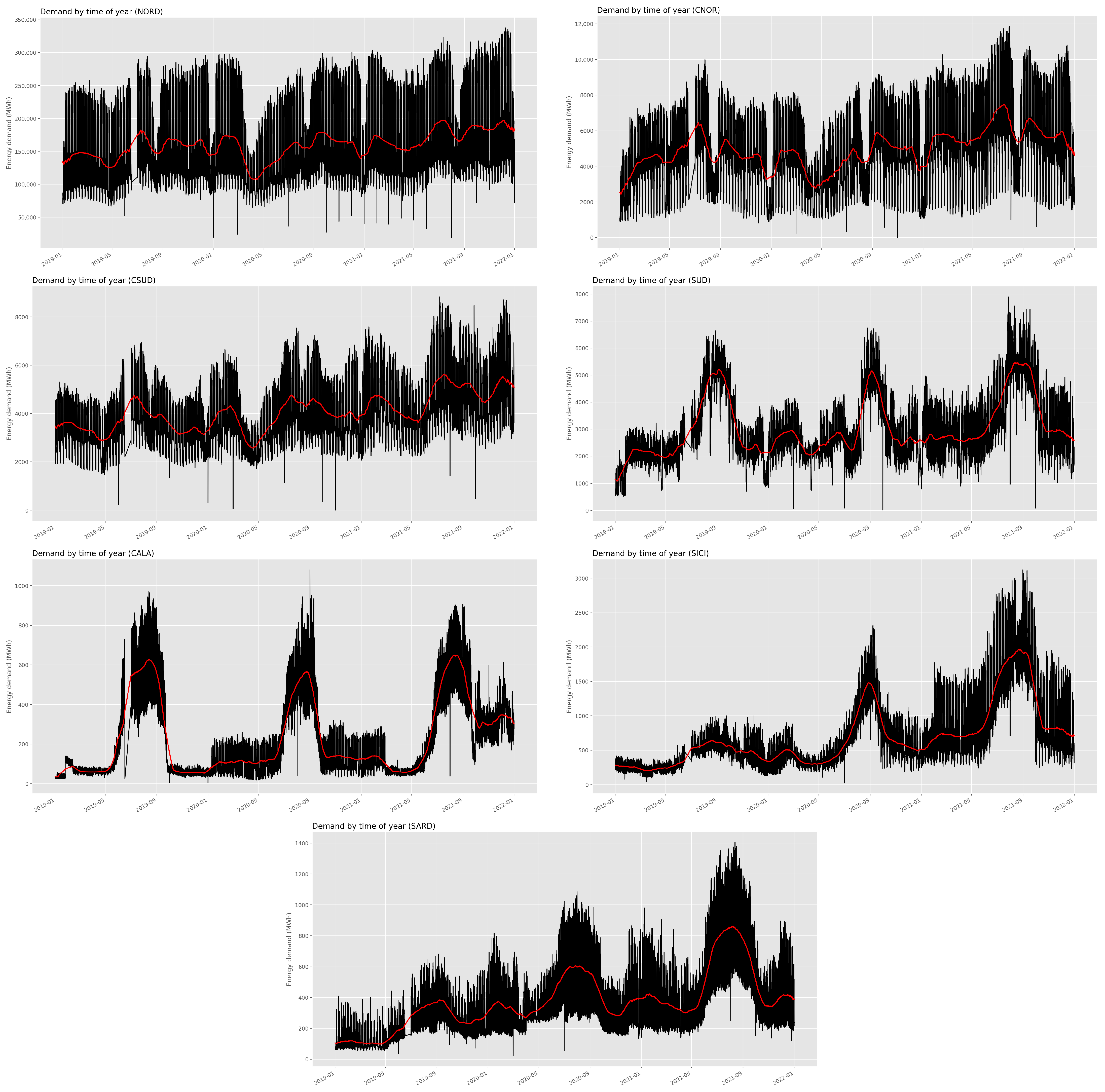
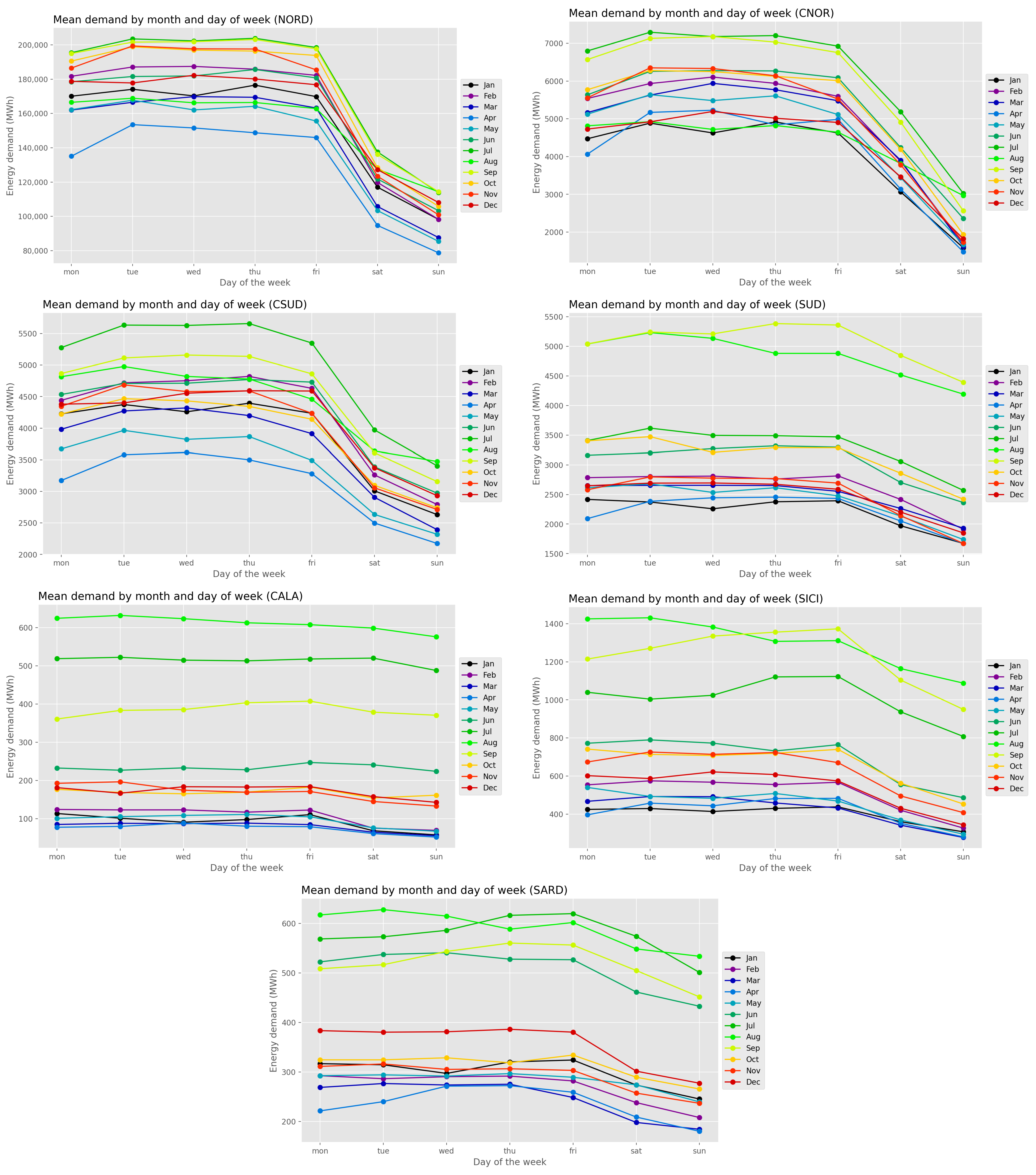
Energy consumption can be affected by several factors, such as, e.g., calendar features. Figure 2 shows a clear time-of-year effect in the data: in NORD, CNOR and CSUD the mean demand is particularly higher in February and July, and lower in April and October; in other words, more energy is needed in winter and summer, whereas fall and spring have a lower demand; we notice a drop in demand in August due to the summer break of many activities. On the other hand, August is the month with the highest demand of the entire year in SUD, CALA, SICI and SARD.
Figure 3 show this trend, with the summer months having the largest average demand in SUD, CALA, SICI and SARD. In the remaining zones, we can see how during the weekend the consumption drops significantly.
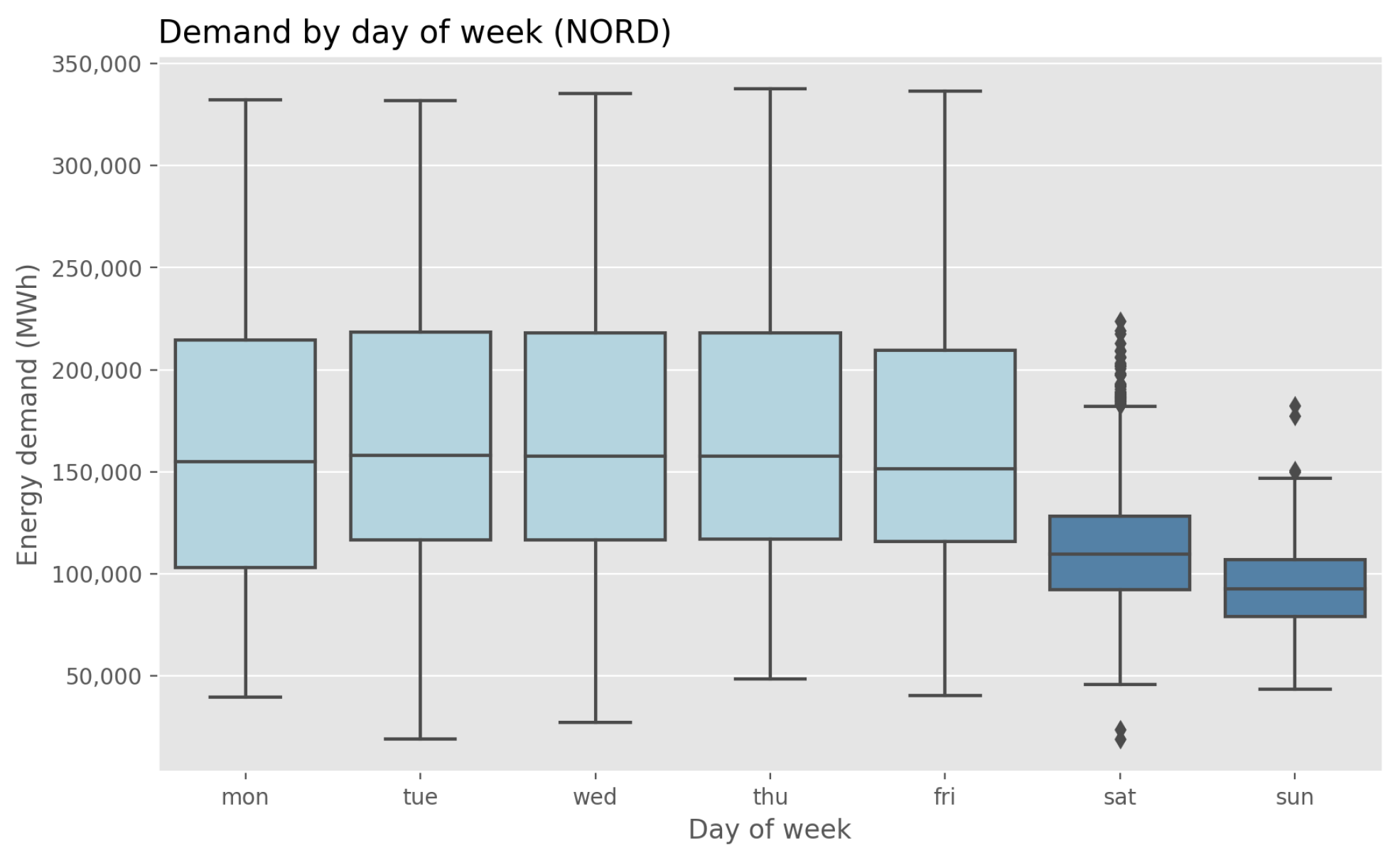
The boxplot in Figure 4 shows how much the energy load is influenced by the day of the week, especially during the weekend when the demand is significantly less.
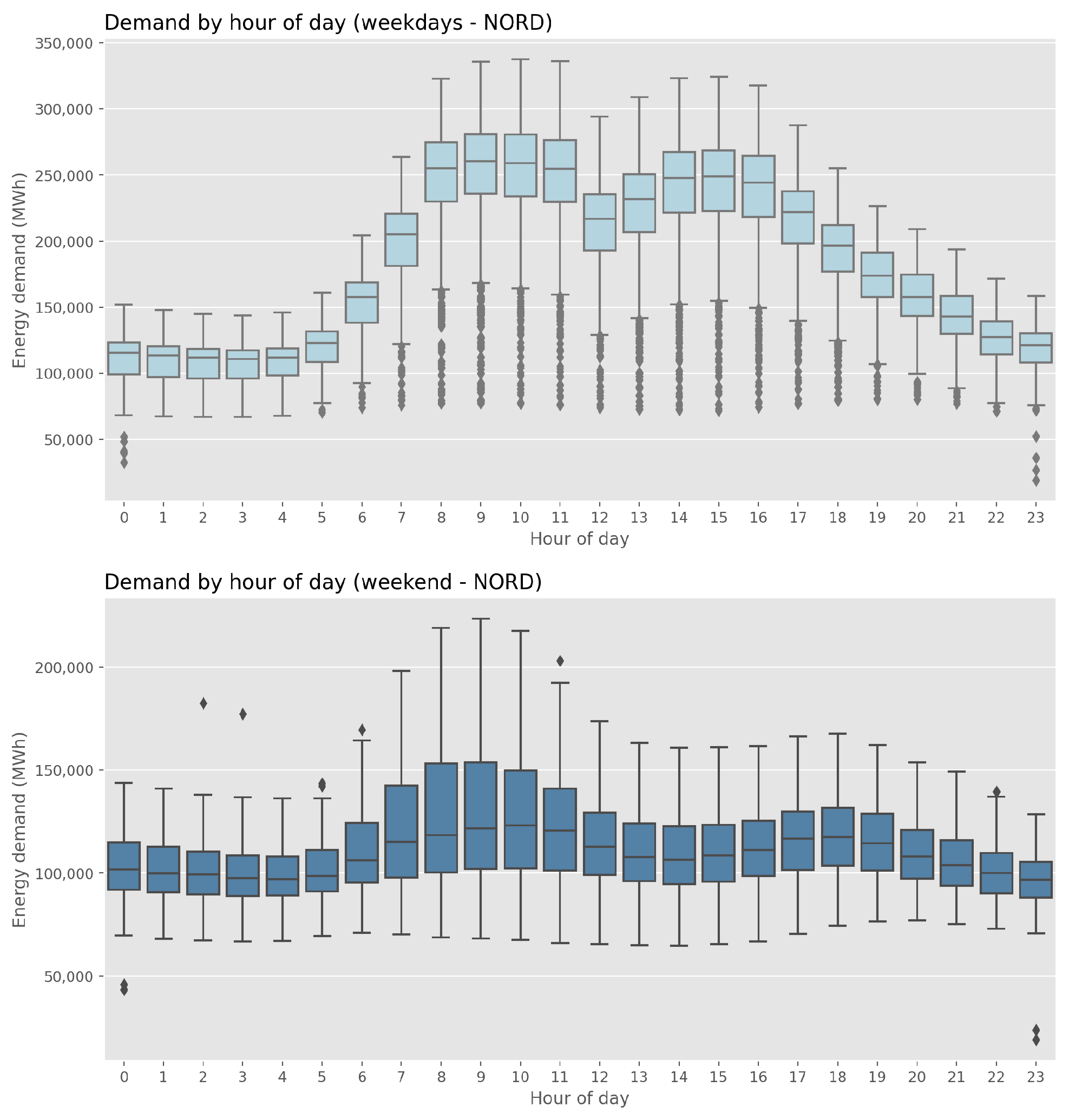
If we take a look at the evolution of the demand throughout the day for a representative zone (see Figure 5), we notice that 9 and 15 are peek hours, while at 3 and 12 we have a local minimum for the demand. These patterns show up softened in the weekend.
Weather conditions, especially air temperature, are likely to influence the consumption of energy. Figure 6 shows the demand in a representative city in Northern Italy plotted against the air temperature in the city is in agreement with what was found earlier. From January to April, as the air temperature gets warmer, the demand for energy decreases. From April to July, there is a positive correlation: when the temperature is hot, the energy demanded is higher. From September to January, as the temperature gets cooler, energy consumption reduces. Overall, the correlation is non-linear, even though the air temperature is an important factor to consider when predicting energy demand.
After the previous exploratory analysis of the dataset, it is convenient to perform some pre-processing steps in order to get rid of missing, repeated or strange values.
First, the leap days have been removed, so that every year is 365 days long.
Second, we identified some outliers in demand. We used a simple algorithm, particularly effective for a series of contiguous outliers. Let x 0 be the value to be checked, x 1 , x 1 the corresponding values of the previous and next week, respectively, and consider their arithmetic mean m : = ( x 1 + x 1 ) / 2 ; we compare x 0 and m, saying that x 0 is an outlier if
| x 0 m | x 0 > k ,
where k is a zone-dependent threshold tuned empirically, by direct observation of the dataset. During the first wave of SARS-CoV-2, the interruption of productive activities and services caused a sudden drop in the demand, especially in the zones NORD, CNOR and CSUD (see Figure 2). The forecasting during that period was extremely challenging and was handled separately. Currently, the data affected by the first wave are not used for training, hence they have been removed but not uniformly in all zones: in CALA, where the impact has been negligible, all data have been kept; in the other zones the data from March to June have been removed; in NORD, also July and August have been taken away.
Finally, we normalize the dataset. The energy load of each client is divided by the maximum power, according to its contract, i.e., the maximum amount of energy in the time unit that can be provided. This allows the model to work with percentages, reducing the unbalance between very big companies and small customers. At the end of the procedure, the data are unnormalized, as we are interested in the absolute amount of energy demanded.

2.2. Model Design

This section describes in abstract terms the model that will be used later to concretely obtain the predictions of the energy demand.

2.2.1. Decision Trees: Base Learner

A decision tree is a hierarchical structure used for classification and regression problems. Every new instance runs through the tree starting from the root and going down one level at a time. For each internal node, a question relative to an attribute is asked, and depending on the outcome a different branch is chosen. This procedure ends when a leaf node, representing a label or a value is reached.
A tree can be learned by optimizing an objective function, usually the entropy to be maximized or a loss-function to be minimized. The training can be interrupted according to an early-stopping criterion.
As a result, the parameter space is divided into distinct and non-overlapping subsets of points with very similar attributes and the same label (or class value).
Decision trees are very reliable methods as they generate understandable rules. In addition, they can handle both continuous and categorical variables simultaneously. The robustness to outliers and to missing data in the input set makes them highly convenient, and due to their hierarchical structure, they automatically perform feature selection, the attributes closest to the root being more important for the prediction.
All these advantages come with a few drawbacks. Firstly, decision trees are more suited for classification rather than regression.
Moreover, decision trees are easily prone to over-fitting: the higher and more complex the tree is constructed, the more it will be dependent on the training data. Finally, sorting every attribute to choose the best one every time we want to generate a new splitting can turn out to be expensive from the computational point of view. For the same reason, pruning techniques, important to avoid over-fitting, can be costly as each time many sub-trees have to be evaluated.
Here comes the idea of ensemble models: instead of training a single big tree, it can be more convenient to build numerous more little trees; any new observation is tested on all the trees and the results are combined in some way (either majority vote or computing the mean). The most popular ensemble models are random forest, bagging and gradient boosting machine. The final result is a collection of trees; what differs is how they are trained. For a random forest, a random subset of attributes is selected to create a new split, but all the data is used. Whereas for bagging, all attributes are considered, but each tree uses a bootstrapped data set from a subset of the whole training set. For both methods, the decision trees are created independently and each one of them contributes equally to the final voting. On the other hand, the trees are built sequentially, as each tree is trained on the errors of the preceding [19].
A more detailed description of this procedure is contained in the following section.

2.2.2. Gradient Boosting Machine

(This section follows the exposition of gradient boosting by Cheng [23].)
The idea behind boosting is to create a sequence of simple models, called weak learners, where every simple model tries to correct the errors made by all the previous models. If the base unit is a decision tree, the final ensemble is referred to as a boosted tree.
Adaptive Boosting (or AdaBoost) was one of the first implementations. The weak learners are called decision stumps, as they are trees with a single split. At first, all the points in the training set are treated equally. When learning a stump, the observation that is harder to classify is given more weight. The following stump will focus more on these difficult instances.
Gradient Boosting takes its name from the fact that it is based on a loss function to minimize (the gradient points in the direction of a greater increase of the function). Each weak learner represents a step towards the minimum.
Let { ( x i , y i ) } i = 1 , , n be the training set. Let us proceed stage-wise:
  • ( m = 0 ) our model F 0 can be simply set to predict the empirical mean:
    F 0 ( x i ) = y ¯ i = 1 , , n .
  • ( m m + 1 ) to improve F m , we add a new estimator h m such that
    F m + 1 ( x i ) = F m ( x i ) + h m ( x i ) = y i i = 1 , , n ,
    that is
    h m ( x i ) = y i F m ( x i ) i = 1 , , n .
    This means that the new estimator h m is found by minimizing the residuals with respect to the previous model F m .
So, gradient boosting could be specialized to a gradient descent algorithm, and generalizing it entails “plugging in” a different loss and its gradient. We refer to (Chapter 10, [29]), for more details. This new estimator h m can be seen as the m-th step towards the minimum of a function, namely the loss function, depending on the residuals. Indeed, if
L = 1 n i = 1 n ( y i F m ( x i ) ) 2 ,
then
L F ( x i ) = 2 n ( y i F m ( x i ) ) = 2 n h m ( x i ) .
The following pseudocode, taken from (Algorithm 1, [20]) describes the method. We refer to the [20] for further details.

2.2.3. GBM Hyperparameters Tuning

Hyperparameters are parameters that describes the structure of the model and allow to regulate the learning process. Hence they are tuned before the actual training. Examples of hyperparameters in the GBM are the maximum number of leaves on the tree and the learning rate η ( 0 , 1 ) , which controls the step size at each iteration. The former is an example of a model hyperparameter, as it defines the actual structure of the tree; the latter is referred to as an algorithm hyperparameter, and it influences the speed of the learning process. Other learning control parameters are the minimum number of data in one leaf; the bagging fraction β , which represents the part of the data that will not be resampled on the next iteration; the bagging frequency (if it is equal to k, it means that every k iterations the algorithm will randomly select β · 100 % of the data to use for the next k iterations); a fraction of features randomly selected to perform each iteration; the coefficient of L 2 -regularization.
For the tuning of the hyperparameters, a separate dataset, namely the validation set, is used to avoid any interference with the learning of the actual model parameters performed on the training set. The validation set will be also used for the early-stopping rule during the training phase.
The hyperparameter optimization consists of creating a model with specific hyperparameter values, and assess its performance on the validation set and retaining the best model.
We can mathematically reformulate this with
θ * = argmin θ f ( x | θ ) ,
where θ denote the vector of hyperparameters, x is any point in the validation set and f is an error function, such as a Root Mean Squared Error (RMSE).
Searching for the optimal θ can be carried out in different ways. With grid search, all the possible combinations of θ are scanned within a bounded space. It is also possible to proceed randomly, by sampling each hyperparameter value according to a preset statistical distribution, i.e., θ is treated as a random variable. However, these methods are quite expensive, as the construction of the model and its testing are intensive tasks. Moreover, past results are not exploited when choosing the next candidate θ . With Bayesian optimization, it is possible to recover past information and speed up the process. The objective function f is treated as a random variable itself, and a prior is placed on it. Then, f is evaluated using the data x , its posterior distribution is updated and its minimizer θ is computed. Then θ is plugged into f and the evaluation takes place once again. We stop when the minimizer is stable.
Bayesian optimization has been used to tune the following hyperparameters: the minimum number of data points in each leaf, the minimum number of leaves in each tree, the coefficient of L 2 -regularization and the learning rate. The values of the remaining hyperparameters have been chosen manually.

2.2.4. Features

The model is enriched with an abundant number of external features, which can be categorized in historical, calendar and meteorological features. To prevent overfitting, a few of them with very low significance are discarded via a backward selection strategy.

Lagged Demand Effects

We incorporate into the model recent demand values as well as the state of the contract of a subset of clients (about 40%) corresponding to the past 7 days. These are the only daily data provided by the energy company, and the reason behind such a fragmented collection of records is technological: different generations of users’ meters send the measurements at a different frequency (the newer versions every 15 min, whereas older versions every hour, day, week, etc.).

Calendar Effects

The calendar features include annual, monthly, weekly and daily patterns, as well as meteorological seasons. Therefore the following features are all included in the model: year, month, day of month, day of week, hour of day, week of year, week of month, day of year, season. To take into account the impact of weekends and festivities, dummy variables are added, indicating whether a day is a Saturday, a Sunday, a holiday, the day before (or after) a holiday. Since the price of the energy depends on the time slot of the day, this feature is also taken into account. Including an increasing and non-repeating feature, such as a timestamp, is helpful whenever a sudden event happens, such as an abrupt change in customer portfolio, or any crisis (coronavirus). Indeed, the model is able to link the anomalous behavior in energy demand to a particular time interval.

Temperature Effects

Due to its correlation with the energy demand, as observed in Section 2.1, the air temperature represent an important feature. Each day the model provided the minimum, average and maximum temperature for the main cities of the zone for the following 4 days. Since we are interested in predicting the aggregate energy demand for each zone, the temperatures of all the sites are potential predictors.

3. Results

3.1. Training and Forecasting

Each model is re-trained monthly, and further checks are performed. For instance, customer portfolios are updated to keep track of the activation of new contracts as well as the termination of older ones.
During the training, a weight strategy is utilized. Each month, m, is assigned a vector of three positive integers ( w m 1 , w m , w m + 1 ) which represent the weights of the previous, current, and future months in relation to the current month. This means that the training errors from each month are multiplied by their corresponding weight, allowing the model to pay more attention to the surrounding months. The weights for each month are determined through a process called cross-validation. To account for the loss of power during wire transportation, we need to provide slightly more energy than requested. This extra amount is reflected in the tension coefficient, which is based on the electric tension (i.e., voltage) of the wire: high, medium, and low tension. Customers have been divided into three groups accordingly. In order to do this with a single model, we need to periodically calculate the tension coefficient as a weighted mean, with the weights being the sum of the maximum power of the customers in each group.
The energy company sends daily three files containing: the forecasts of the minimum, maximum and average air temperature of the main cities for the next 7 days, the state of the contracts and the demand of a subset of clients (about 40%) relative to the past 7 days, also called “D-7”. As previously explained, the partial information is caused by the electric meters sending measurements at different frequencies. The D-7 turns out to be very inconsistent and unstable over time, making it extremely important to normalize it with respect to the maximum power and the average composition of the customers’ portfolio in terms of high, medium, and low tension.

3.2. Numerical Results

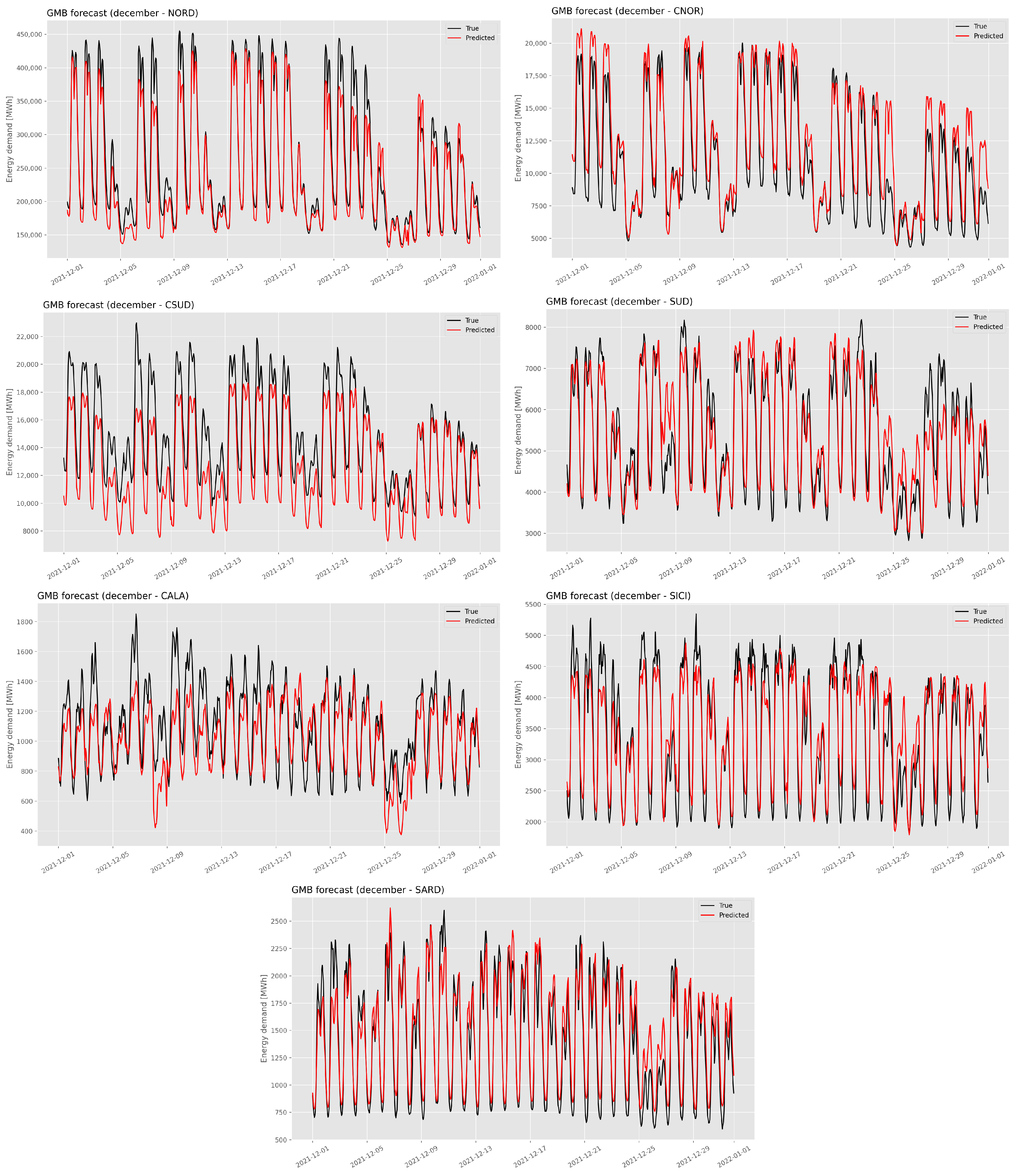
The free and open-source distributed gradient boosting framework LightGBM, originally developed by Microsoft (https://github.com/microsoft/LightGBM, accessed on 6 December 2022), has been imported and used. The code was developed by customizing the library and implementing the training routine as introduced in the previous section. Every day, the hourly 4-day-ahead forecasting of energy demand is produced for every zone. However, only the 1-day-ahead prediction is used for error evaluation once the energy company provides the true energy load consumption for the entire customer’s portfolio (approximately two months after the prediction). The metric used by the energy company to evaluate the performance of the software is the Mean Absolute Percentage Error (MAPE). The reason for using this metric is two-fold: first, it places greater emphasis on penalizing overestimations compared to underestimations, which is desirable as overestimations result in wasted energy and money. Second, the metric of Mean Absolute Percentage Error (MAPE) is the one used by the energy company itself to evaluate the accuracy of predictions. The dataset used for training ranges from January 2019 to October 2021, while November and December 2021 were used for testing. These months have been chosen to assess the behavior of the model both in a normal and regular month, such as November, and in a month with short (8 December) and long (24–31 December) holidays, such as December. The predictions are displayed in Figure 7 and Figure 8.
The value of MAPE for each zone is reported in Table 1. The model is very accurate in NORD and SUD where the MAPE stays below 10% in November and December. In CSUD the model has the tendency to underestimate the energy load demand. This is partly because of the metric adopted for training: for the same absolute deviation from the true value, the MAPE put more weight on the overestimation rather than the underestimation [30]. This results in a slightly biased model, and the issue can be softened by suitably correcting the metric [31]. Another possible reason can be found in the anomalous decrease in the demand - not present in the previous two years - right before the testing months (Figure 2). CNOR has the opposite problem in December, as the predictions appear slightly above the true values, especially during the Christmas holidays. In CALA, SICI and SARD the model struggles to capture the more irregular pattern of the load demand. This could be partly caused by the limited size of the customers’ portfolio, as most of the clients are based in Northern regions. In addition, a modification in the composition of the portfolio may lead to some troubles in the forecasting procedure. As an example, both from Figure 9 and Figure 2 we can see that the number of clients and the average demand in CALA has risen in October, November and December 2021, compared to the same period of 2020. This results in an underestimation that can be adjusted by giving more importance to the feature indicating the number of active clients. This, together with the correction of the error metric, could be the subject of future research.

3.3. Feature Importance Analysis

As the GBM is based on a random-tree architecture, an analysis of the feature importance can be performed easily. As said in Section 2.2.4, a small subset of the features has already been discarded. However, another feature importance procedure is carried out during the training: when building a tree, we count the number of times each feature is used; the most informative features are chosen more often.
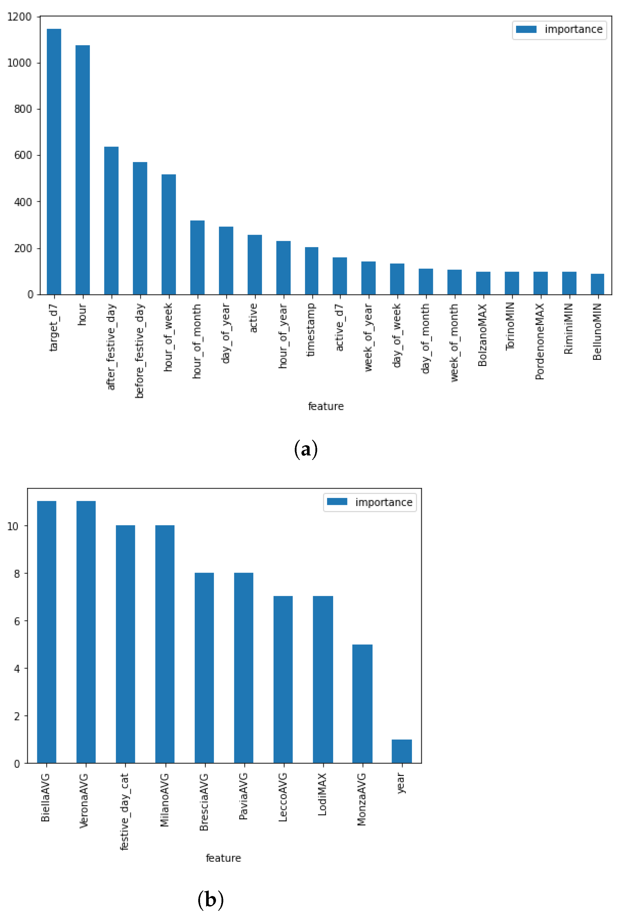
Figure 10 shows the most and least useful features used by the model. It is no surprise that the most important feature is the consumption seven days before the prediction. The second most important is the hour of the day, as the consumption varies a lot during each day. We can notice that many other calendar features have been considered more helpful than the meteorological features, especially the dummies for the day before or after a holiday. Among the least useful features we find at the end of the year, maybe because the training set is only 2-year-long.

3.4. Comparison with Classical Statistical Models

In this section, we compare the performance of the GBM model with a traditional statistical model, namely an ARMA model on the remainder resulting from the decomposition of the time series. We conduct this simulation in NORD, as it is the region where GBM has demonstrated the highest performance. The time series decomposition has been carried out as follows: the trend has been fitted as a polynomial of degree 1 through the Least Squared method; the de-trended series has been differentiated at lag 24 (1 day), lag 168 (7 days) and lag 1 (1 h), the most significant periodicities emerged from the periodogram; the resulting series is the remainder; the seasonal component has been obtained subtracting the remainder to the de-trended series. In the remainder, we fitted an ARMA( p , q ), where p and q are also chosen with a model selection procedure based on Akaike’s Information Criterion. The training has been conducted using the Python libraries statsmodels and scipy.
Both November and December have been predicted and the MAPE has been computed and compared with GBM in Table 2. GBM outperforms ARMA in both months, especially in December. We can see from Figure 11 how ARMA is not sensitive to holidays, having a regular seasonal component that is not affected by calendar features. It is not possible to model this behavior in the remainder, as a stationarity assumption needs to hold. One possibility could be to add an additional component encoding the information about weekends and holidays.

4. Conclusions

In the present paper, we addressed the fundamental task in energy trading markets of energy load forecasting.
After a few pre-processing steps, a deeper analysis of the correlation between energy loads and external regressors, such as calendar features and air temperature, has been conducted. In particular, the latter has shown to be an extremely important feature to be considered for energy load forecasting. The dependence is non-linear and not uniform throughout the year.
That is why a non-linear framework such as the Gradient Boosting Decision Tree model has been adopted for the forecasting task.
Despite that the most recent complete data are two months old and the data provided daily involve only a heterogeneous subset of the entire customer’s portfolio, itself quite fragmented in the first place due to the different versions of the electric meters, the model has proved to be able to exploit the 7-day-before information in an optimal way: the normalization with respect to the maximum power is essential to recover the actual structure of the time series.
The experimental results show that the GBM model has significantly better performances compared to classical statistical methods, such as ARMA models. The GBM model has been able to learn the multiple inner periodic behaviors, such as seasonal, weekly and daily fluctuations, as well as the influence of weekends and holidays. The MAPE ranges around 10–15%, according to the market zone, but can reach levels of 5% in NORD, where the dataset is bigger. The main drawbacks of the model are that it systematically underestimates performance, which is caused by both the error metric used and changes in the customer’s portfolio, and it struggles to accurately predict high and low peaks. To address the first issue, future research should focus on analyzing the magnitude of the underestimation over time for each region. The second issue will be further investigated by studying the factors that most impact predictions during peak hours, which will be carried out in future work.

Author Contributions

Conceptualization, L.D.P. and N.F.; methodology, L.D.P. and N.F.; software, L.D.P.; validation, L.D.P. and N.F.; formal analysis, L.D.P. and N.F.; investigation, L.D.P. and N.F.; resources, L.D.P.; data curation, N.F.; writing—original draft preparation, L.D.P. and N.F.; writing—review and editing, L.D.P. and N.F.; visualization, L.D.P. and N.F.; supervision, L.D.P.; project administration, L.D.P. and N.F. All authors have read and agreed to the published version of the manuscript.

Funding

The authors would like to thank HPA s.r.l. for hospitality and hardware support.

Data Availability Statement

Data sharing not applicable. No new data were created or analyzed in this study. Data sharing is not applicable to this article.

Acknowledgments

This paper has been developed under the European Union (EU) NOP—Research and Innovation aegis, data and code having been partially provided by HPA s.r.l (https://www.hpa.ai, accessed on 3 February 2023).

Conflicts of Interest

The authors declare no conflict of interest.

References

  1. Weron, R. Modeling and Forecasting Electricity Loads and Prices: A Statistical Approach; John Wiley & Sons: Hoboken, NJ, USA, 2007; Volume 403. [Google Scholar]
  2. Lin, Y.; Luo, H.; Wang, D.; Guo, H.; Zhu, K. An ensemble model based on machine learning methods and data preprocessing for short-term electric load forecasting. Energies 2017, 10, 1186. [Google Scholar] [CrossRef] [Green Version]
  3. Pappas, S.S.; Ekonomou, L.; Karampelas, P.; Karamousantas, D.; Katsikas, S.; Chatzarakis, G.; Skafidas, P. Electricity demand load forecasting of the Hellenic power system using an ARMA model. Electr. Power Syst. Res. 2010, 80, 256–264. [Google Scholar] [CrossRef]
  4. Bindiu, R.; Chindris, M.; Pop, G. Day-ahead load forecasting using exponential smoothing. Acta Marisiensis. Ser. Technol. 2009, 6, 89. [Google Scholar]
  5. Nalcaci, G.; Özmen, A.; Weber, G.W. Long-term load forecasting: Models based on MARS, ANN and LR methods. Cent. Eur. J. Oper. Res. 2019, 27, 1033–1049. [Google Scholar] [CrossRef]
  6. Kuster, C.; Rezgui, Y.; Mourshed, M. Electrical load forecasting models: A critical systematic review. Sustain. Cities Soc. 2017, 35, 257–270. [Google Scholar] [CrossRef]
  7. Zhang, J. Research on power load forecasting based on the improved elman neural network. Chem. Eng. Trans. 2016, 51, 589–594. [Google Scholar]
  8. Edwards, R.E.; New, J.; Parker, L.E. Predicting future hourly residential electrical consumption: A machine learning case study. Energy Build. 2012, 49, 591–603. [Google Scholar] [CrossRef]
  9. Chae, Y.T.; Horesh, R.; Hwang, Y.; Lee, Y.M. Artificial neural network model for forecasting sub-hourly electricity usage in commercial buildings. Energy Build. 2016, 111, 184–194. [Google Scholar] [CrossRef]
  10. Amarasinghe, K.; Marino, D.L.; Manic, M. Deep neural networks for energy load forecasting. In Proceedings of the 2017 IEEE 26th International Symposium on Industrial Electronics (ISIE), Edinburgh, UK, 19–21 June 2017; pp. 1483–1488. [Google Scholar]
  11. Feng, C.; Sun, M.; Zhang, J. Reinforced deterministic and probabilistic load forecasting via Q-learning dynamic model selection. IEEE Trans. Smart Grid 2019, 11, 1377–1386. [Google Scholar] [CrossRef]
  12. Cai, L.; Gu, J.; Jin, Z. Two-layer transfer-learning-based architecture for short-term load forecasting. IEEE Trans. Ind. Informatics 2019, 16, 1722–1732. [Google Scholar] [CrossRef]
  13. Hong, T.; Pinson, P.; Wang, Y.; Weron, R.; Yang, D.; Zareipour, H. Energy forecasting: A review and outlook. IEEE Open Access J. Power Energy 2020, 7, 376–388. [Google Scholar] [CrossRef]
  14. Fan, S.; Chen, L.; Lee, W.J. Short-term load forecasting using comprehensive combination based on multimeteorological information. IEEE Trans. Ind. Appl. 2009, 45, 1460–1466. [Google Scholar] [CrossRef]
  15. Fan, S.; Hyndman, R.J. Short-term load forecasting based on a semi-parametric additive model. IEEE Trans. Power Syst. 2011, 27, 134–141. [Google Scholar] [CrossRef] [Green Version]
  16. Rodríguez-Rodríguez, I.; González Vidal, A.; Ramallo González, A.P.; Zamora, M.Á. Commissioning of the controlled and automatized testing facility for human behavior and control (CASITA). Sensors 2018, 18, 2829. [Google Scholar] [CrossRef] [Green Version]
  17. Vartholomaios, A.; Karlos, S.; Kouloumpris, E.; Tsoumakas, G. Short-term renewable energy forecasting in greece using prophet decomposition and tree-based ensembles. In Proceedings of the International Conference on Database and Expert Systems Applications; Springer: Berlin/Heidelberg, Germany, 2021; pp. 227–238. [Google Scholar]
  18. Zhoul, L.; Chenl, M.; Ni, Q. A hybrid prophet-LSTM model for prediction of air quality index. In Proceedings of the 2020 IEEE Symposium Series on Computational Intelligence (SSCI), Canberra, Australia, 1–4 December 2020; pp. 595–601. [Google Scholar]
  19. Touzani, S.; Granderson, J.; Fernandes, S. Gradient boosting machine for modeling the energy consumption of commercial buildings. Energy Build. 2018, 158, 1533–1543. [Google Scholar] [CrossRef] [Green Version]
  20. Friedman, J.H. Greedy function approximation: A gradient boosting machine. Ann. Stat. 2001, 1189–1232. [Google Scholar] [CrossRef]
  21. Zhang, Y.; Haghani, A. A gradient boosting method to improve travel time prediction. Transp. Res. Part C Emerg. Technol. 2015, 58, 308–324. [Google Scholar] [CrossRef]
  22. Ayaru, L.; Ypsilantis, P.P.; Nanapragasam, A.; Choi, R.C.H.; Thillanathan, A.; Min-Ho, L.; Montana, G. Prediction of outcome in acute lower gastrointestinal bleeding using gradient boosting. PLoS ONE 2015, 10, e0132485. [Google Scholar] [CrossRef]
  23. Chen, Y.; Jia, Z.; Mercola, D.; Xie, X. A gradient boosting algorithm for survival analysis via direct optimization of concordance index. Comput. Math. Methods Med. 2013, 2013, 873595. [Google Scholar] [CrossRef] [Green Version]
  24. Lu, H.; Cheng, F.; Ma, X.; Hu, G. Short-term prediction of building energy consumption employing an improved extreme gradient boosting model: A case study of an intake tower. Energy 2020, 203, 117756. [Google Scholar] [CrossRef]
  25. Nie, P.; Roccotelli, M.; Fanti, M.P.; Ming, Z.; Li, Z. Prediction of home energy consumption based on gradient boosting regression tree. Energy Rep. 2021, 7, 1246–1255. [Google Scholar] [CrossRef]
  26. Xie, J.; Coggeshall, S. Prediction of transfers to tertiary care and hospital mortality: A gradient boosting decision tree approach. Stat. Anal. Data Min. Asa Data Sci. J. 2010, 3, 253–258. [Google Scholar] [CrossRef]
  27. Wang, Y.; Feng, D.; Li, D.; Chen, X.; Zhao, Y.; Niu, X. A mobile recommendation system based on logistic regression and gradient boosting decision trees. In Proceedings of the 2016 international joint conference on neural networks (IJCNN), Vancouver, BC, Canada, 24–29 July 2016; pp. 1896–1902. [Google Scholar]
  28. Friedman, J.H.; Meulman, J.J. Multiple additive regression trees with application in epidemiology. Stat. Med. 2003, 22, 1365–1381. [Google Scholar] [CrossRef]
  29. Hastie, T.; Tibshirani, R.; Friedman, J.H.; Friedman, J.H. The Elements of Statistical Learning: Data Mining, Inference, and Prediction; Springer: Berlin/Heidelberg, Germany, 2009; Volume 2. [Google Scholar]
  30. Makridakis, S. Accuracy measures: Theoretical and practical concerns. Int. J. Forecast. 1993, 9, 527–529. [Google Scholar] [CrossRef]
  31. Tofallis, C. A better measure of relative prediction accuracy for model selection and model estimation. J. Oper. Res. Soc. 2015, 66, 1352–1362. [Google Scholar] [CrossRef] [Green Version]
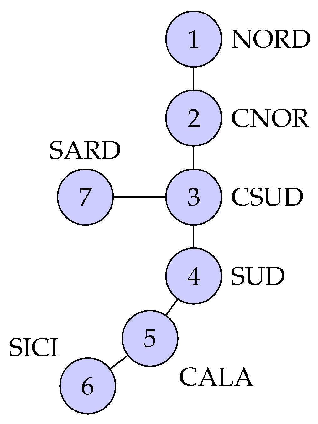
Figure 1. Electricity market zones in Italy.
Mathematics 11 01068 g001
Figure 2. Energy demand plotted against the time of year. The smoothed mean demand is shown as a red line.
Mathematics 11 01068 g002
Figure 3. Average demand of energy by month and day of the week.
Mathematics 11 01068 g003
Figure 4. Boxplot of the energy demand by day of the week in NORD.
Mathematics 11 01068 g004
Figure 5. Boxplot of the energy demand by hour of the day for weekdays and weekends in NORD.
Mathematics 11 01068 g005
Figure 6. Hourly load vs. hourly air temperature in a representative city in Northern Italy.
Mathematics 11 01068 g006
Figure 7. Prediction of GBM model for November 2021.
Mathematics 11 01068 g007
Figure 8. Prediction of the GBM model for December 2021.
Mathematics 11 01068 g008
Figure 9. Number of active clients in each zone.
Mathematics 11 01068 g009
Figure 10. Feature importance for NORD. (a) Most important features. (b) Least important features.
Mathematics 11 01068 g010
Figure 11. Forecasts using time series decomposition and ARMA model for November and December.
Mathematics 11 01068 g011
Table 1. MAPE (%) for the GBM predictions of November and December.
NovemberDecember
NORD5.098.00
CNOR7.8314.71
CSUD12.0913.61
SUD6.898.43
CALA14.6413.03
SICI13.699.30
SARD12.2111.79
Table 2. MAPE for ARMA and GBM for November and December.
NovemberDecember
ARMA8.3617.15
GBM5.098.00
Disclaimer/Publisher’s Note: The statements, opinions and data contained in all publications are solely those of the individual author(s) and contributor(s) and not of MDPI and/or the editor(s). MDPI and/or the editor(s) disclaim responsibility for any injury to people or property resulting from any ideas, methods, instructions or products referred to in the content.