A New Reciprocal Weibull Extension for Modeling Extreme Values with Risk Analysis under Insurance Data

Abstract

Probability-based distributions might be able to explain risk exposure well. Usually, one number, or at the very least, a limited number of numbers called the key risk indicators (KRIs), are used to describe the level of risk exposure. These risk exposure values, which are undeniably the outcome of a specific model, are frequently referred to as essential critical risk indicators. Five key risk indicators, including value-at-risk, tail variance, tail-value-at-risk, and tail mean-variance, were also used for describing the risk exposure under the reinsurance revenues data. These measurements were created for the proposed model; hence, this paper presents a novel distribution for this purpose. Relevant statistical properties are derived, including the generating function, ordinary moments, and incomplete moments. Special attention is devoted to the applicability of the new model under extreme data sets. Three applications to real data show the usefulness and adaptability of the proposed model. The new model proved its superiority against many well-known related models. Five key risk indicators are employed for analyzing the risk level under the reinsurance revenues dataset. An application is provided along with its relevant numerical analysis and panels. Some useful results are identified and highlighted.

1. Introduction and Motivation

Actuarial risks refer to the financial risks associated with insurance and pension plans. Statistical analysis is an important tool for actuaries to understand and quantify these risks. Actuaries use probability distributions to model the likelihood of various events, such as claims, deaths, and policy cancellations. Common distributions used in actuarial science include the Poisson distribution, the exponential distribution, and the Weibull distribution. Survival analysis is used to model the time until a particular event occurs, such as death or policy cancellation. This technique is used to estimate the probability of survival for a given time period and to calculate life expectancy. Stochastic modeling is used to model random processes, such as claims and policy cancellations. This technique is used to estimate the expected value of future claims and to determine the variability of these estimates. Loss distributions are used to model the distribution of losses due to events, such as claims and policy cancellations. This technique is used to calculate the expected value of future losses and to determine the risk associated with these losses. Actuaries use statistical techniques used to assess and manage financial risks, including methods for hedging and portfolio optimization.

In conclusion, statistical analysis is a critical tool for actuaries to understand and manage financial risks in insurance and pension plans. Actuaries use a variety of statistical techniques, including probability distributions, survival analysis, stochastic modeling, loss distributions, and risk management, to estimate and manage financial risks and ensure the long-term financial stability of insurance and pension plans.

Because they depict situations where extreme occurrences or outliers occur far more frequently than expected by traditional or lighter-tailed distributions, such as the normal distribution, heavy-tailed probability distributions are significant. Numerous real-world systems, including financial markets, communication networks, and natural disasters, may be significantly impacted by these occurrences. To effectively reflect the risk and uncertainty associated with such severe events and to make decisions based on the probabilities of these events, it is crucial to comprehend and model heavy-tailed distributions.

In the actuarial and statistical literature, the issue of measuring the risk resulting from some accidents is considered a matter of great importance. This is because determining the level of risk and measuring its degree will entail a lot of strategic actions and decisions. One of the most important fields in which we, as statisticians, are interested in measuring risk is the field of insurance and reinsurance and the field of actuarial sciences in general. Insurance companies, for example, are very interested in anticipating the volume of claims that they may be bound by soon. Statistical prediction of the volume of claims will make the insurance company stable for a certain period of time. Thus, if the expectations are correct, the company will be in a safe position with the insured parties. Additionally, if it is not correct, then the company will be in a safer position in most cases.

Based on the importance of this issue, whether in terms of actuarial modeling or in terms of statistical forecasts, we are excited about this work as it presents a flexible probabilistic model to help insurance and reinsurance companies determine the volume of claims that may occur in the near future. The new probability model is a probability distribution that presents many characteristics that contributed to its nomination to this actuarial task.

The issue of measuring risk has attracted the attention of many researchers in recent decades. The researchers’ interests focused on presenting and generalizing some actuarial indicators that may contribute to measuring risk under certain conditions. These indicators varied in their forms according to the statistical basis on which they were built. Some depend on the quantile function; some depend on moments; some depend on the tail of the probability distribution, and so on.

Heavy-tailed probability-based distributions refer to probability distributions that have “heavier” tails than the normal distribution, meaning that they have a higher probability of observing extreme values (outliers). This is in contrast to light-tailed distributions, such as the normal distribution, where the probability of observing extreme values is low. Examples of heavy-tailed distributions include; the Pareto distribution, which is used to model the distribution of wealth and income and is characterized by a long tail on the right side of the distribution; the Student’s t-distribution, which is used in hypothesis testing and has heavier tails than the normal distribution, making it more suitable for modeling data with outliers; the Lévy distribution, which is used in financial mathematics and physics and has heavier tails than the normal distribution; and the Cauchy distribution, which has infinite variance and is used to model phenomena with long tails, such as response times in networks and earthquakes.

Heavy-tailed distributions are important in many fields, including finance, economics, physics, and engineering, as they provide a more accurate representation of real-world phenomena where extreme events are more common than expected under a normal distribution. Heavy tailed probability-based distributions might be capable of explaining risk exposure well. Normally, one number, or at the very least a limited number of numbers, is used to describe the level of risk exposure. The term “crucial KRIs” refers to these risk exposure figures, which are undeniably the output of a certain model (see Artzner [1] and Wirch [2]). Such KRIs give actuaries and risk managers knowledge about the level of a company’s exposure to particular risks. There are many KRIs that can be considered and studied, including value-at-risk (VAR), tail-value-at-risk (TVAR), conditional-value-at-risk (CVAR), tail variance (TV), and tail Mean-Variance (TMV), among others. The VAR is specifically included in the quantile distribution of aggregate losses. Actuaries and risk managers usually concentrate on calculating the chance of a bad outcome, which can be measured using the VAR indicator at a particular probability/confidence level. This indicator is typically used to estimate how much money will be required to handle such potentially unfavorable events. The ability of the insurance firm to handle such events is a worry for actuaries, policymakers, investors, and rating agencies.

For this purpose, a novel probability-based reciprocal Weibull distribution called the generalized geometric Rayleigh reciprocal Weibull (GGR-RW) is provided for an adequate explanation of risk exposure under the reinsurance revenues data set. The probability density function (PDF) and cumulative distribution function (CDF) of the reciprocal Weibull (RW) distribution are given by

$$g_{{\delta }_1,{\delta }_2}(𝓎)={\delta }_1^{{\delta }_2}{\delta }_2{𝓎}^{-\left({\delta }_2+1\right)}exp\left(-{\delta }_1^{{\delta }_2}{𝓎}^{-{\delta }_2}\right) {|}_{𝓎\ge 0},$$

and

$$G_{{\delta }_1,{\delta }_2}(𝓎)=exp\left(-{\delta }_1^{{\delta }_2}{𝓎}^{-{\delta }_2}\right) {|}_{𝓎\ge 0},$$

where ${\delta }_2>0$ is a shape parameter and ${\delta }_1>0$ is a scale parameter. For ${\delta }_2=2$, we obtain the reciprocal Rayleigh (RR) model. For ${\delta }_2=1,$ we obtain the reciprocal exponential (RE) model, and for ${\delta }_1=1$, we obtain the one parameter reciprocal Weibull (1PRW) model. Let $g_{{\delta }_1,{\delta }_2}(𝓎)$ and $G_{{\delta }_1,{\delta }_2}(𝓎)$ denote the PDF and CDF of the RW model with parameters ${\delta }_1$ and ${\delta }_2$ and consider the CDF of the generalized Rayleigh (GR) family, then the CDF of the generalized Rayleigh reciprocal Weibull (GR-RW) model

$$H_{b,{\delta }_1,{\delta }_2}(𝓎)=1-exp\left[-{\nabla }_{b,{\delta }_1,{\delta }_2}^2(𝓎)\right]{|}_{𝓎\ge 0;b>0},$$

(1)

where

$${\nabla }_{b,{\delta }_1,{\delta }_2}(𝓎)=\frac{exp\left(-b{\delta }_1{𝓎}^{-{\delta }_2}\right)}{1-exp\left(-b{\delta }_1{𝓎}^{-{\delta }_2}\right)}{|}_{𝓎\ge 0,b>0},$$

and ${𝓀}_{b,{\delta }_1,{\delta }_2}(𝓎)=d{H}_{b,{\delta }_1,{\delta }_2}(𝓎)/d𝓎$ is the PDF corresponding to (1). For any arbitrary baseline RV having CDF$,$ and $\underset{\_}{\mathbb{V}}$ representing the baseline parameters vector, then the CDF of the geometric family is defined by

$$F_{a,\underset{\_}{\mathbb{V}}}(𝓎)=\frac{a{H}_{\underset{\_}{\mathbb{V}}}(𝓎)}{1-\left(1-a\right)H_{\underset{\_}{\mathbb{V}}}(𝓎)}{|}_{𝓎\in R;a>0}.$$

(2)

Then, the new model is derived by combining (1) and (2). The CDF of the GGR-RW model can be defined by

$$F_{\underset{\_}{\mathit{\varphi }}}(𝓎)=\frac{a-aexp\left[-{\nabla }_{b,{\delta }_1,{\delta }_2}^2(𝓎)\right]}{1-\left(1-a\right)\left\{1-exp\left[-{\nabla }_{b,{\delta }_1,{\delta }_2}^2(𝓎)\right]\right\}}{|}_{𝓎\ge 0;a,b,{\delta }_1,{\delta }_2>0},$$

(3)

where $\underset{\_}{\mathit{\varphi }}=\left(a,b,{\delta }_1,{\delta }_2\right)$ refers to the parameter vector. Then, the PDF corresponding to (3) is

$$f_{\underset{\_}{\mathit{\varphi }}}(𝓎)=2ab{\delta }_1^{{\delta }_2}{\delta }_2{𝓎}^{-\left({\delta }_2+1\right)}exp\left(-2{\delta }_1^{{\delta }_2}b{𝓎}^{-{\delta }_2}\right)\frac{{\left[1-exp\left(-b{\delta }_1^{{\delta }_2}{𝓎}^{-{\delta }_2}\right)\right]}^{-3}exp\left[-{\nabla }_{b,{\delta }_1,{\delta }_2}^2(𝓎)\right]}{{\left(1-\left(1-a\right)\left\{1-exp\left[-{\nabla }_{b,{\delta }_1,{\delta }_2}^2(𝓎)\right]\right\}\right)}^2}{|}_{𝓎\ge 0,a>0,b>0}.$$

(4)

Using the generalized binomial expansion and the power series, the PDF in (4) can be expressed as

$$f_{\underset{\_}{\mathit{\varphi }}}(𝓎)=2ab{\delta }_1^{{\delta }_2}{\delta }_2{𝓎}^{-\left({\delta }_2+1\right)}exp\left(-{\delta }_1^{{\delta }_2}{𝓎}^{-{\delta }_2}\right){\displaystyle \sum }_{𝒾,𝒿,\ell =0}^{\infty }\frac{{\left(1-a\right)}^{𝒾}{\left(-1\right)}^{\ell }}{\ell !{\left(1+𝒾\right)}^{-\ell }}\frac{exp\left\{-\left[2b\left(\ell +1\right)-1\right]{\delta }_1^{{\delta }_2}{𝓎}^{-{\delta }_2}\right\}}{{\left[1-exp\left(-b{\delta }_1^{{\delta }_2}{𝓎}^{-{\delta }_2}\right)\right]}^{3+2\ell }}\left(\begin{array}{c}-2\\ 𝒾\end{array}\right)\left(\begin{array}{c}𝒾\\ 𝒿\end{array}\right)$$

Using Taylor expansion, we can write

$$f_{\underset{\_}{\mathit{\varphi }}}(𝓎)={\displaystyle \sum }_{\ell ,𝓂=0}^{\infty }{c}_{\ell ,𝓂}\hspace{0.17em}{g}_{b\left[2\left(\ell +1\right)+𝓂\right],{\delta }_1,{\delta }_2}(𝓎){|}_{b\left[2\left(\ell +1\right)+𝓂\right]>0},$$

(5)

where

$$c_{\ell ,𝓂}=2ab{\displaystyle \sum }_{𝒾=0}^{\infty }{\displaystyle \sum }_{𝒾=0}^{𝒿}\frac{{\left(1-a\right)}^{𝒾}{\left(-1\right)}^{\ell }{\left(1+𝒾\right)}^{\ell }}{\ell !b\left[2\left(\ell +1\right)+𝓂\right]}\left(\begin{array}{c}-2\\ 𝒾\end{array}\right)\left(\begin{array}{c}𝒾\\ 𝒿\end{array}\right)\left(\begin{array}{c}-3-2\ell \\ 𝓂\end{array}\right),$$

and

$$G_{b\left[2\left(\ell +1\right)+𝓂\right],{\delta }_1,{\delta }_2}(𝓎)=b\left[2\left(\ell +1\right)+𝓂\right]{\delta }_1^{{\delta }_2}{\delta }_2{𝓎}^{-\left({\delta }_2+1\right)}exp\left(-b\left[2\left(\ell +1\right)+𝓂\right]{\delta }_1^{{\delta }_2}{𝓎}^{-{\delta }_2}\right)$$

refers to the RW density with scale parameter ${\delta }_1$ ${\left\{b\left[2\left(\ell +1\right)+𝓂\right]\right\}}^{\left(1/{\delta }_2\right)}$ and shape parameter ${\delta }_2.$ Thus, some mathematical properties of the GGR-RW model can be obtained simply from those properties of the RW density. The CDF of the GGR-RW model can also be expressed as a mixture of RW densities. By integrating (5), we obtain the same mixture representation

$$F_{\underset{\_}{\mathit{\varphi }}}(𝓎)={\displaystyle \sum }_{\ell ,𝓂=0}^{\infty }{c}_{\ell ,𝓂}{G}_{b\left[2\left(\ell +1\right)+𝓂\right],{\delta }_1,{\delta }_2}(𝓎){|}_{b\left[2\left(\ell +1\right)+𝓂\right]>0},$$

(6)

where $G_{b\left[2\left(\ell +1\right)+𝓂\right],{\delta }_1,{\delta }_2}(𝓎)=exp\left(-b\left[2\left(\ell +1\right)+𝓂\right]{\delta }_1^{{\delta }_2}{𝓎}^{-{\delta }_2}\right)$ is the CDF of the RW model with scale parameter ${\delta }_1$ ${\left\{b\left[2\left(\ell +1\right)+𝓂\right]\right\}}^{\left(1/{\delta }_2\right)}$ and shape parameter ${\delta }_2$. In fact, the GGR-RW model is motivated by its important flexibility in applications. We demonstrate that the GGR-RW model offers better fits than many other competing models using three applications. The “asymmetric monotonically increasing hazard rate function (HRF)” shown in Figure 1 suggests that the GGR-RW model could be beneficial in real-life modeling data (first row, right panels).

The GGR-RW model can be recommended for modeling real data which have some extreme values. Also, the GGR-RW model could be useful for analyzing and modeling real data which has no extreme observations, as shown in Figure 7 (the second row of the right and the left panels). Moreover, the GGR-RW distribution can be considered a useful model for modeling real data for which its nonparametric Kernel density is symmetric and unimodal. The GGR-RW could be a good choice for dealing with the real data which its nonparametric Kernel density is the asymmetric bimodal and heavy tail, as illustrated in Figure 1, Figure 4 (the first row, left panels). Finally, the GGR-RW model may be useful in modeling the real data which cannot be fitted by the common theoretical distributions, such as normal, uniform, exponential, logistic, beta, lognormal, and Weibull distributions as illustrated in Figure 1.

The rest of the paper is organized as follows. We derive a few mathematical features for the new model in Section 2. Some risk indicators are discussed in Section 3. We introduce the maximum likelihood technique in Section 4. We present three applications to actual data in Section 5 to demonstrate the adaptability of the new family. Section 6 provides the risk analysis for the reinsurance revenues data. Finally, Section 6 addresses a few closing thoughts.

2. Properties

The ${𝓇}^{th}$ moment of $Y$, say ${\mu }_{𝓇,Y}^{\prime }$, follows from (5) as ${\mu }_{𝓇,Y}^{\prime }=E\left(Y^{𝓇}\right)={\displaystyle \sum }_{\ell ,𝓂=0}^{\infty }{c}_{\ell ,𝓂}E\left(Y_{\left\{b\left[2\left(\ell +1\right)+𝓂\right]\right\}}^{𝓇}\right).$

Henceforth, $Y_{\left\{b\left[2\left(\ell +1\right)+𝓂\right]\right\}}$ denotes the RW distribution with scale parameter ${\delta }_1$ ${\left\{b\left[2\left(\ell +1\right)+𝓂\right]\right\}}^{\left(1/{\delta }_2\right)}$ and shape parameter ${\delta }_2$. Then, we have

$$E\left(Y_{\left\{b\left[2\left(\ell +1\right)+𝓂\right]\right\}}^{𝓇}\right)={\delta }_1^{{\delta }_2}{\delta }_2\left\{b\left[2\left(\ell +1\right)+𝓂\right]\right\}{{\displaystyle \int }}_0^{\infty }{𝓎}^{-\left({\delta }_2+1\right)+𝓇}exp\left(-\left\{b\left[2\left(\ell +1\right)+𝓂\right]\right\}{\delta }_1^{{\delta }_2}{𝓎}^{-{\delta }_2}\right)d𝓎,$$

Then,

$${\mu }_{𝓇,Y}^{\prime }=E\left(Y^{𝓇}\right)=\mathsf{\Gamma }\left(1-\frac{𝓇}{{\delta }_2}\right){\displaystyle \sum }_{\ell ,𝓂=0}^{\infty }{c}_{\ell ,𝓂}{\left({\delta }_1 {\left\{b\left[2\left(\ell +1\right)+𝓂\right]\right\}}^{\left(1/{\delta }_2\right)}\right)}^{𝓇},$$

(7)

the numerical value of the constant ${{\displaystyle \sum }}_{\ell ,𝓂=0}^{\infty }{c}_{\ell ,𝓂}{\left({\delta }_1 {\left\{b\left[2\left(\ell +1\right)+𝓂\right]\right\}}^{\left(1/{\delta }_2\right)}\right)}^{𝓇}$ can be evaluated using any software such as R and MATHCAD among others. The moment generating function (MGF) $M_Y(𝓉)=E\left(exp\left(𝓉Y\right)\right)$ of $Y$ can be derived from Equation (5) as

$$M_Y(𝓉)={\displaystyle \sum }_{\ell ,𝓂=0}^{\infty }{c}_{\ell ,𝓂}{M}_{\left\{b\left[2\left(\ell +1\right)+𝓂\right]\right\},{\delta }_1,{\delta }_2}(𝓉),$$

where $M_{\left\{b\left[2\left(\ell +1\right)+𝓂\right]\right\},{\delta }_1,{\delta }_2}(𝓉)$ is the MGF of $Y_{\left\{b\left[2\left(\ell +1\right)+𝓂\right]\right\}}$. Hence,

$$M_Y(𝓉)=\mathsf{\Gamma }\left(1-\frac{𝓇}{{\delta }_2}\right){\displaystyle \sum }_{\ell ,𝓂,𝓇=0}^{\infty }\frac{c_{\ell ,𝓂}}{𝓇!}{\left(𝓉{\delta }_1 {\left\{b\left[2\left(\ell +1\right)+𝓂\right]\right\}}^{\left(1/{\delta }_2\right)}\right)}^{𝓇}.$$

The $s^{th}$ incomplete moment, say ${\mathit{\varphi }}_{s,Y}(𝓉)$, of $Y$ can be expressed from (5) as

$${\mathit{\varphi }}_{s,Y}(𝓉)={{\displaystyle \int }}_{-\infty }^{𝓉}{𝓎}^s{f}_{\underset{\_}{\mathit{\varphi }}}(𝓎)d𝓎={\displaystyle \sum }_{\ell ,𝓂=0}^{\infty }{c}_{\ell ,𝓂}{I}_{-\infty }^{𝓉}\left({𝓎}^s;\left\{b\left[2\left(\ell +1\right)+𝓂\right]\right\},{\delta }_1,{\delta }_2\right),$$

where $I_{-\infty }^{𝓉}\left({𝓎}^s;\left\{b\left[2\left(\ell +1\right)+𝓂\right]\right\},{\delta }_1,{\delta }_2\right)={{\displaystyle \int }}_0^{𝓉}{𝓎}^s{g}_{\left\{b\left[2\left(\ell +1\right)+𝓂\right]\right\},{\delta }_1,{\delta }_2}(𝓎)d𝓎.$ Then,

$${\mathit{\varphi }}_{s,Y}(𝓉)={\displaystyle \sum }_{\ell ,𝓂=0}^{\infty }{c}_{\ell ,𝓂}{\left({\delta }_1 {\left\{b\left[2\left(\ell +1\right)+𝓂\right]\right\}}^{\left(1/{\delta }_2\right)}\right)}^{𝓇}\gamma \left(1-\frac{𝓇}{{\delta }_2},\left\{b\left[2\left(\ell +1\right)+𝓂\right]\right\}{\delta }_1^{{\delta }_2}{𝓉}^{-{\delta }_2}\right).$$

(8)

The $n^{th}$ moment of the residual life of $Y$ is given by

$${𝓂}_{n,Y}(𝓉)=\frac{1}{1-F_{\underset{\_}{\mathit{\varphi }}}(𝓉)}{\displaystyle \sum }_{\ell ,𝓂=0}^{\infty }{\displaystyle \sum }_{𝓇=0}^n{c}_{\ell ,𝓂}\left(\begin{array}{c}n\\ 𝓇\end{array}\right){\left(-𝓉\right)}^{n-𝓇}{I}_{𝓉}^{\infty }\left({𝓎}^n;\left\{b\left[2\left(\ell +1\right)+𝓂\right]\right\},{\delta }_1,{\delta }_2\right),$$

where

$$I_{𝓉}^{\infty }\left({𝓎}^n;\left\{b\left[2\left(\ell +1\right)+𝓂\right]\right\},{\delta }_1,{\delta }_2\right)={{\displaystyle \int }}_{𝓉}^{\infty }{𝓎}^n{g}_{\left\{b\left[2\left(\ell +1\right)+𝓂\right]\right\}}(𝓎)d𝓎$$

then,

$$I_{𝓉}^{\infty }\left({𝓎}^n;\left\{b\left[2\left(\ell +1\right)+𝓂\right]\right\},{\delta }_1,{\delta }_2\right)={\left({\delta }_1 {\left\{b\left[2\left(\ell +1\right)+𝓂\right]\right\}}^{\left(1/{\delta }_2\right)}\right)}^n\mathsf{\Gamma }\left(1-\frac{n}{{\delta }_2},\left\{b\left[2\left(\ell +1\right)+𝓂\right]\right\}{\delta }_1^{{\delta }_2}{𝓉}^{-{\delta }_2}\right).$$

The $n^{𝓉𝓀}$ moment of the reversed residual life, say $M_{n,Y}(𝓉)=E\left[{(𝓉-Y)}^n\hspace{0.17em}|\hspace{0.17em}Y\le 𝓉\right]$ for $𝓉>0$ and $n=1, 2$,…, follows as $M_{n,Y}(𝓉)=\frac{1}{F_{\underset{\_}{\mathit{\varphi }}}(𝓉)}{{\displaystyle \int }}_0^{𝓉}{(𝓉-𝓎)}^{n}dF(𝓎).$ Therefore, the $n$^th moment of the reversed residual life of $Y$ becomes

$$M_{n,Y}(𝓉)=\frac{1}{F_{\underset{\_}{\mathit{\varphi }}}(𝓉)}{\displaystyle \sum }_{\ell ,𝓂=0}^{\infty }{\displaystyle \sum }_{𝓇=0}^n{c}_{\ell ,𝓂}{\left(-1\right)}^{𝓇}\left(\begin{array}{c}n\\ 𝓇\end{array}\right){𝓉}^{n-𝓇}{I}_0^{𝓉}\left({𝓎}^n;\left\{b\left[2\left(\ell +1\right)+𝓂\right]\right\},{\delta }_1,{\delta }_2\right),$$

where

$$I_0^{𝓉}\left({𝓎}^n;\left\{b\left[2\left(\ell +1\right)+𝓂\right]\right\},{\delta }_1,{\delta }_2\right)={{\displaystyle \int }}_0^{𝓉}{𝓎}^n{g}_{b^{*}}(𝓎)d𝓎$$

then,

$$I_0^{𝓉}\left({𝓎}^n;\left\{b\left[2\left(\ell +1\right)+𝓂\right]\right\},{\delta }_1,{\delta }_2\right)={\left({\delta }_1 {\left\{b\left[2\left(\ell +1\right)+𝓂\right]\right\}}^{\left(1/{\delta }_2\right)}\right)}^n$$

$$\times \gamma \left(1-\frac{n}{{\delta }_2},\left\{b\left[2\left(\ell +1\right)+𝓂\right]\right\}{\delta }_1^{{\delta }_2}{𝓉}^{-{\delta }_2}\right).$$

3. KRIs

The KRIs are metrics that use statistical methods to measure and monitor an organization’s key risks. KRSIs are a type of KRIs that use statistical techniques, such as probability distributions, regression analysis, and hypothesis testing, to provide a quantitative and data-driven assessment of risk. These KRIs measure the frequency and magnitude of losses due to various risks, such as accidents, losses due to fraud, or losses due to natural disasters. An actuarial estimate of the possible loss that could arise in the future as a result of a particular action or set of circumstances is the risk exposure. Risks are often assessed according to their likelihood of happening in the future multiplied by the potential loss if they did as part of a review of the business’s risk exposure. By assessing the possibility of future losses, a company can distinguish between small and significant losses. Speculative risks frequently lead to losses, including failing to adhere to regulations, a decrease in brand value, security vulnerabilities, and liability issues.

The examination of historical insurance data using time series analysis or continuous distributions has, nevertheless, received a great deal of attention. Actuaries have recently used continuous distributions, especially ones with broad tails, to represent actual insurance data. Using continuous heavy-tailed probability distributions, real data has been modeled in a number of real-world applications, including engineering, risk management, dependability, and the actuarial sciences. The skewness of the insurance data sets can be left, right, or right with huge tails.

Risk exposure is an inevitable event for any insurance firm. Actuaries developed a variety of risk indicators to measure risk exposure as a result. The VAR indicator determines the risk of a potential loss for the insurance company with a specified probability and calculates the amount that a group of investments could lose. An increasingly popular benchmark risk metric for determining risk exposure is this indicator. The VAR often determines how much capital is required, given a specific likelihood, to ensure that the business will not officially go out of business. The chosen confidence level is arbitrary. As a result, a significant VAR amount may be considered for various confidence levels. For the entire company, it may be a high proportion, for example, 99.95% or greater. The inter-unit or inter-risk type of diversification that exists can be represented by these different percentages.

In this paper, these five insurance indicators were chosen due to their importance and prevalence in the statistical literature. These five indicators can express the size of the expected loss for insurance companies and, thus, help insurance companies avoid unexpected and sudden random losses. In insurance analysis, loss refers to the amount of money an insurance company must pay to an insured individual or business as a result of a covered event or claim. Losses can include things such as property damage, medical expenses, and liability judgments. The calculation of loss is a crucial aspect of the insurance industry, as it helps insurance companies determine the financial risks of providing coverage and determine the rates charged for insurance policies.

3.1. VAR Indicator

The VAR is a financial metric that measures the maximum loss that an investment or portfolio is expected to experience with a certain level of confidence over a specified time period. VAR is used to quantify market risk and is a widely used risk management tool for financial institutions. The VAR indicator provides a single value that summarizes the potential loss of an investment or portfolio. This method uses historical data to simulate the distribution of returns and estimate the VAR for a portfolio. This method uses statistical models, such as the normal distribution or the GARCH model, to estimate the VAR for a portfolio. The VAR is a useful risk management tool, as it provides a clear and concise measure of the potential loss of an investment or portfolio. However, it has limitations, as it only provides a point estimate of the potential loss and does not take into account tail risks or extreme events. To address these limitations, financial institutions often use other risk management tools in conjunction with VAR, such as stress testing and scenario analysis.

Definition 1.

Let $Y$ denote a loss random variable, The VAR of $Y$ at the $100\epsilon \%$ level, say VAR $\left(Y\right)$ or $p\left(\epsilon \right)$, is the $100\epsilon \%$ quantile (or the $100\epsilon \%$ percentile ($Q_Y$)) of the distribution of $Y$.

Then, based on Definition 1 for the GGR-RW distribution, we can simply write

$$\stackrel{}{Pr}\left(Y>Q_Y\right)=\{\begin{array}{c}1\%{|}_{\epsilon =99\%}\\ 5\%{|}_{\epsilon =95\%}\\ ⋮\end{array},$$

From Definition 1, for a one-year time when $\epsilon =90\%$, the interpretation is that there is only a very small chance ($10\%$) that the insurance company will be bankrupted by an adverse outcome over the next year. The quantity VAR $\left(Y;\epsilon \right)$ does not satisfy one of the five criteria for coherence (see Wirch [2]).

3.2. TVAR Risk Indicator

The VAR indicator is frequently used as a risk assessment tool in the management of financial risk over a defined relatively short time period. Gains and losses are commonly explained in these circumstances using the normal distribution.

The quantity VAR $\left(Y;\epsilon \right)$ satisfies all coherence requirements if the distribution of gains (or losses) is restricted to the normal distribution.

Definition 2.

Let$Y$denote a random loss variable, then the TVAR of$Y$at the$100\epsilon \%$confidence level is the expected loss given that the loss exceeds the$100\epsilon \%$of the distribution of$Y$can be expressed as

$$\mathrm{TVAR}\left(Y\right)=E\left(Y|Y⟩p\left(\epsilon \right)\right)=\frac{1}{1-F_{\underset{\_}{\mathit{\varphi }}}\left(p\left(\epsilon \right)\right)}{{\displaystyle \int }}_{p\left(\epsilon \right)}^{\infty }𝓎f_{\underset{\_}{\mathit{\varphi }}}(𝓎)d𝓎=\frac{1}{1-\epsilon }{{\displaystyle \int }}_{p\left(\epsilon \right)}^{\infty }𝓎f_{\underset{\_}{\mathit{\varphi }}}(𝓎)d𝓎.$$

Then,

$$\mathrm{TVAR}\left(Y\right)=\frac{1}{1-\epsilon } I_{p\left(\epsilon \right)}^{\infty }\left(𝓎;\left\{b\left[2\left(\ell +1\right)+𝓂\right]\right\},{\delta }_1,{\delta }_2\right),$$

where $I_{p\left(\epsilon \right)}^{\infty }\left(𝓎;\left\{b\left[2\left(\ell +1\right)+𝓂\right]\right\},{\delta }_1,{\delta }_2\right)={{\displaystyle \int }}_{p\left(\epsilon \right)}^{\infty }𝓎g_{\left\{b\left[2\left(\ell +1\right)+𝓂\right]\right\},{\delta }_1,{\delta }_2}(𝓎)d𝓎.$ Then,

$$\mathrm{TVAR}\left(Y\right)=\frac{ {\delta }_1}{1-\epsilon }{\left\{b\left[2\left(\ell +1\right)+𝓂\right]\right\}}^{\left(1/{\delta }_2\right)}{\displaystyle \sum }_{\ell ,𝓂=0}^{\infty }{c}_{\ell ,𝓂}\mathsf{\Gamma }\left(1-\frac{1}{{\delta }_2},\left\{b\left[2\left(\ell +1\right)+𝓂\right]\right\}{\delta }_1^{{\delta }_2}{\left(p\left(\epsilon \right)\right)}^{-{\delta }_2}\right).$$

(9)

Thus, the quantity in (9) is an average of all VAR values above at the confidence level $\epsilon$, which provides more information about the tail of the GGR-RW distribution. Further, it can also be expressed as

$$\mathrm{TVAR}\left(Y;\epsilon \right)=\mathrm{VAR}\left(Y;\epsilon \right)+l\left(\mathrm{VAR}\left(Y;\epsilon \right)\right),$$

where $l\left(\mathrm{VAR}\left(Y;\epsilon \right)\right)$ is the mean excess loss function evaluated at the $100\epsilon \%$ th quantile. So, TVAR $\left(Y;\epsilon \right)$ is larger than its corresponding VAR $\left(Y;\epsilon \right)$ by the amount of average excess of all losses that exceed the EL $\left(Y;\epsilon \right)$ value of VAR $\left(Y;\epsilon \right)$. The VAR $\left(Y;\epsilon \right)$ has been independently developed and is also known as the conditional tail expectation in the insurance literature (Wirch [2]). According to Tasche [3] and Acerbi and Tasche [4], it has also been referred to as the expected shortfall (ES) or the conditional tail expectation (TCE).

3.3. TV Risk Indicator

Furman and Landsman [5] established the TV risk indicator, which determines the loss’s departure from the mean along a tail. Furman and Landsman [6] have created explicit calculations for the TV risk indicator under the multivariate normal distribution.

Definition 3.

Let$Y$denote a random loss variable, then the TV risk indicator (TR($Y$)) can be expressed as

$$\mathrm{TV}\left(Y;\epsilon \right)=E\left(Y^2|Y⟩p\left(\epsilon \right)\right)-{\left[\mathrm{TVAR}\left(Y;\epsilon \right)\right]}^2.$$

Then,

$$\mathrm{TV}\left(Y;\epsilon \right)=\frac{{\left[{\delta }_1{\left\{b\left[2\left(\ell +1\right)+𝓂\right]\right\}}^{\left(1/{\delta }_2\right)}\right]}^2}{1-\epsilon }{\displaystyle \sum }_{\ell ,𝓂=0}^{\infty }{c}_{\ell ,𝓂}\left\{{\mathsf{\omega }}_{p\left(\epsilon \right)}\left(2;{\delta }_1,{\delta }_2\right)-\frac{ 1}{1-\epsilon }{\left[{\mathsf{\omega }}_{p\left(\epsilon \right)}\left(1;{\delta }_1,{\delta }_2\right)\right]}^2\right\},$$

(10)

where

$${\mathsf{\omega }}_{p\left(\epsilon \right)}\left(\nabla ;{\delta }_1,{\delta }_2\right)=\mathsf{\Gamma }\left(1-\frac{\nabla }{{\delta }_2},\left\{b\left[2\left(\ell +1\right)+𝓂\right]\right\}{\delta }_1^{{\delta }_2}{\left(p\left(\epsilon \right)\right)}^{-{\delta }_2}\right).$$

Thus, the quantities in (9) and (10) can be evaluated using any software such as R and MATHCAD, among others, and we will give a numerical example under the reinsurance data with all details and panels in Section 6.

3.4. TMV Risk Indicator

As a metric for the best portfolio choice, Landsman [5] developed the TMV risk indicator, which is based on the TCE risk indicator and the TV risk indicator.

Definition 4.

Let$Y$denote a random loss variable, then the TMV risk indicator can be expressed as

$$\mathrm{TMV}\left(Y;\epsilon \right)=\mathrm{TVAR}\left(Y;\epsilon \right)+p\mathrm{TV}\left(Y;\epsilon \right){|}_{0<p<1}.$$

Then, for any LRV

• the TMV $\left(Y;\epsilon \right)>$ TV $\left(Y;\epsilon \right)$,
• for $p=0$, TMV $\left(Y;\epsilon \right)=$ TVAR $\left(Y;\epsilon \right)$,
• for $p=1$, TMV $\left(Y;\epsilon \right)=$ TVAR $\left(Y;\epsilon \right)+$ TV $\left(Y;\epsilon \right).$

4. Modeling

Both simulation and real data have their advantages and disadvantages when comparing models. Using simulation data allows for complete control over the underlying data-generating process and enables the researcher to systematically vary the parameters and compare the models under different conditions. This can provide insight into the robustness and generalizability of the models. On the other hand, using real data provides a more realistic evaluation of the models as it reflects real-world scenarios and allows for the evaluation of the model’s ability to handle real-world complexities and uncertainties. Ultimately, the choice between simulation and real data will depend on the research question, the purpose of the comparison, and the availability of data. In many cases, a combination of both simulation and real data can provide a more comprehensive evaluation of the models being compared.

To illustrate the wide flexibility of the GGR-RW model, we considered three real-life data sets, and the new model is compared with many other relevant and competitive models. Table 1 reports some of the competitive models (see Fréchet [7], Nadarajah and Kotz [8], and Krishna et al. [9]). Real-life data can be examined quantitatively, visually, or using both methods. In order to examine the first fit to theoretical distributions, such as the normal, uniform, exponential, logistic, beta, lognormal, and Weibull distributions, we will take into consideration a variety of graphical tools, including the skewness-kurtosis panel (or the Cullen and Frey panel). For more accuracy, bootstrapping is applied. The Cullen and Frey panel summarizes the characteristics of distribution by comparing distributions in the space of squared skewness and kurtosis. The “nonparametric Kernel density estimation (NKDE)” approach for examining initial density shape, the “Quantile-Quantile (Q-Q)” panel for examining the “normality” of the data, the “total time in test (TTT)” panel for examining the initial shape of the empirical HRFs, the “box panel” for examining the extremes, and the scattergrams are also paneled, which are all taken into consideration.

Table 1. Some competitive models.

Competitive Models (Author(s))	Abbreviation
reciprocal Weibull	RW
exponentiated reciprocal Weibull	E-RW
Beta reciprocal Weibull model	Beta-RW
Marshal-Olkin reciprocal Weibull	MO-RW
transmuted reciprocal Weibull model	T-RW
Kumaraswamy reciprocal Weibull	Kum-RW
McDonald reciprocal Weibull	Mc-RW
odd log-logistic reciprocal Rayleigh	OLL-RR
odd log-logistic exponentiated reciprocal Weibull	OLLE-RW
odd log-logistic exponentiated reciprocal Rayleigh	OLLE-RR
generalized odd log-logistic reciprocal Rayleigh	GOLL-RR

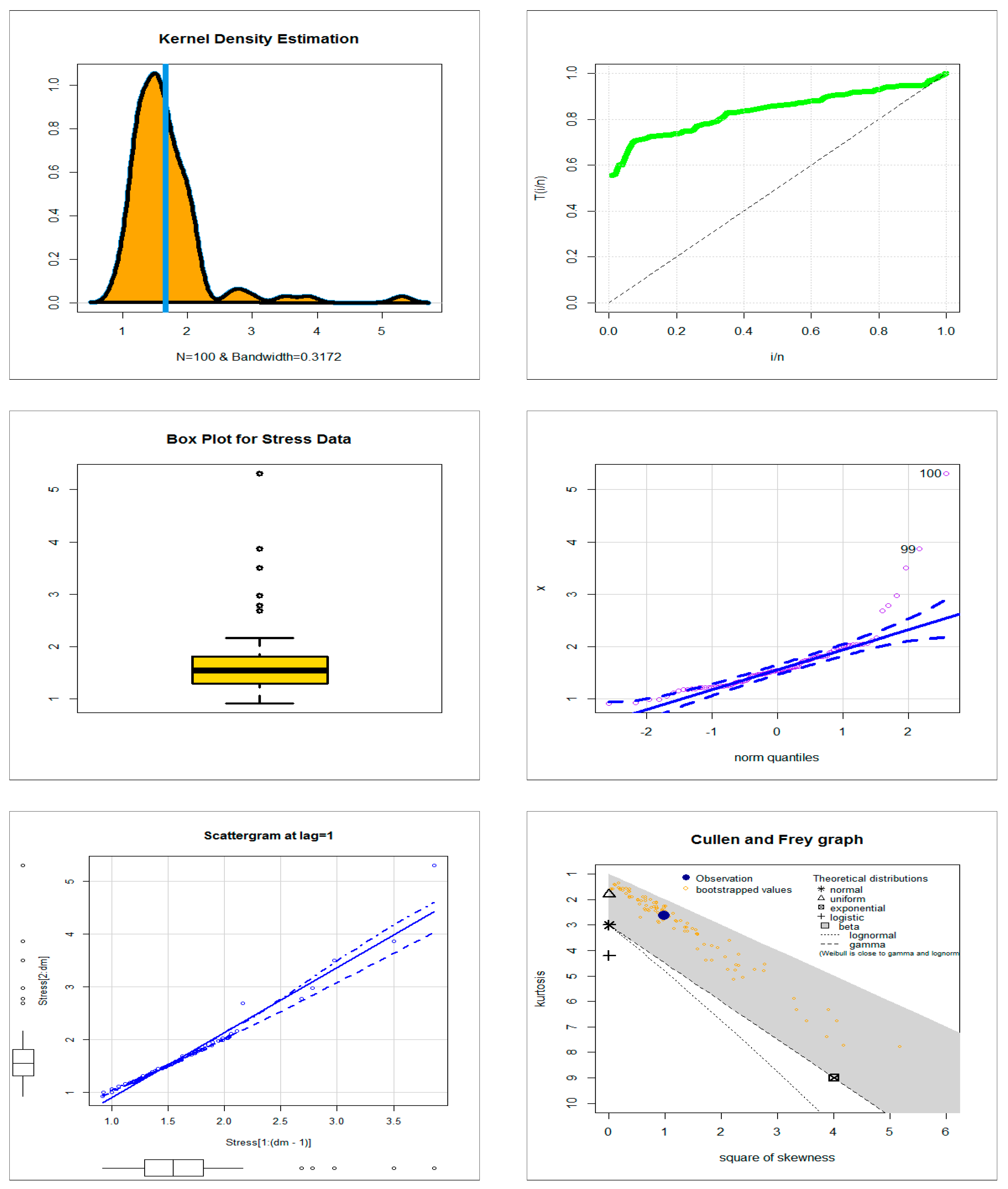
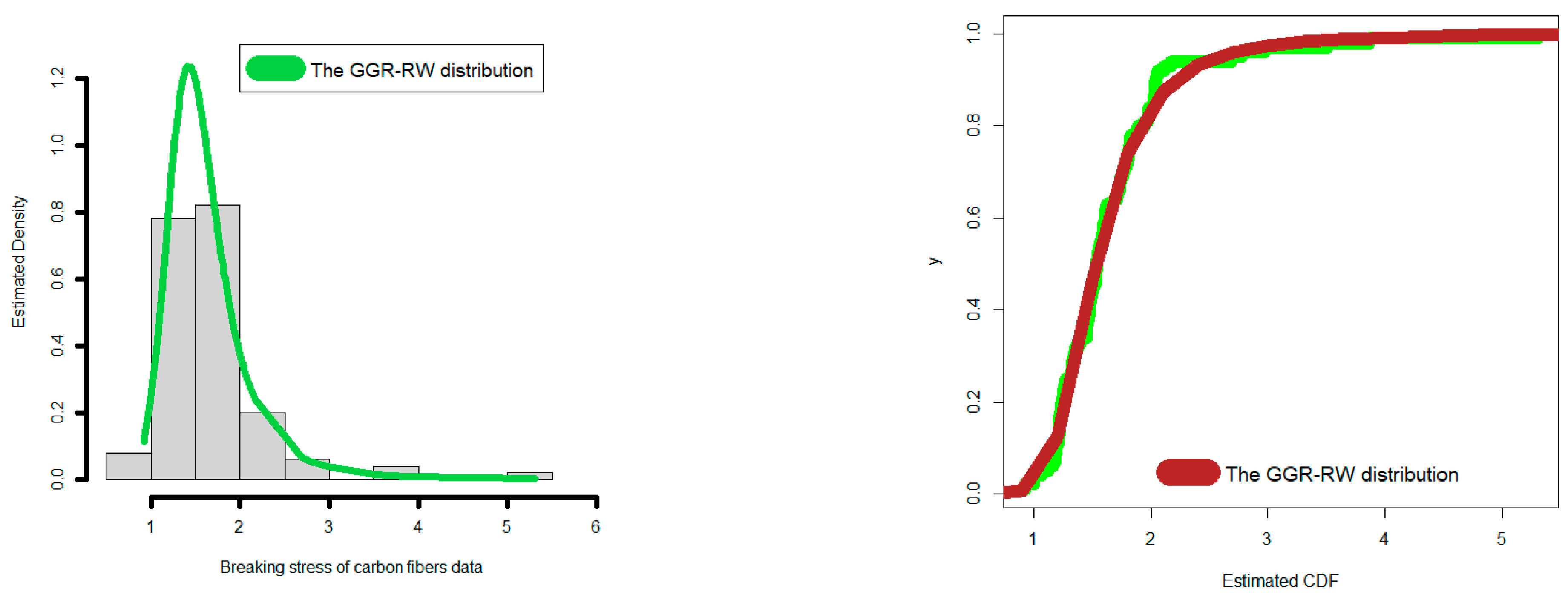
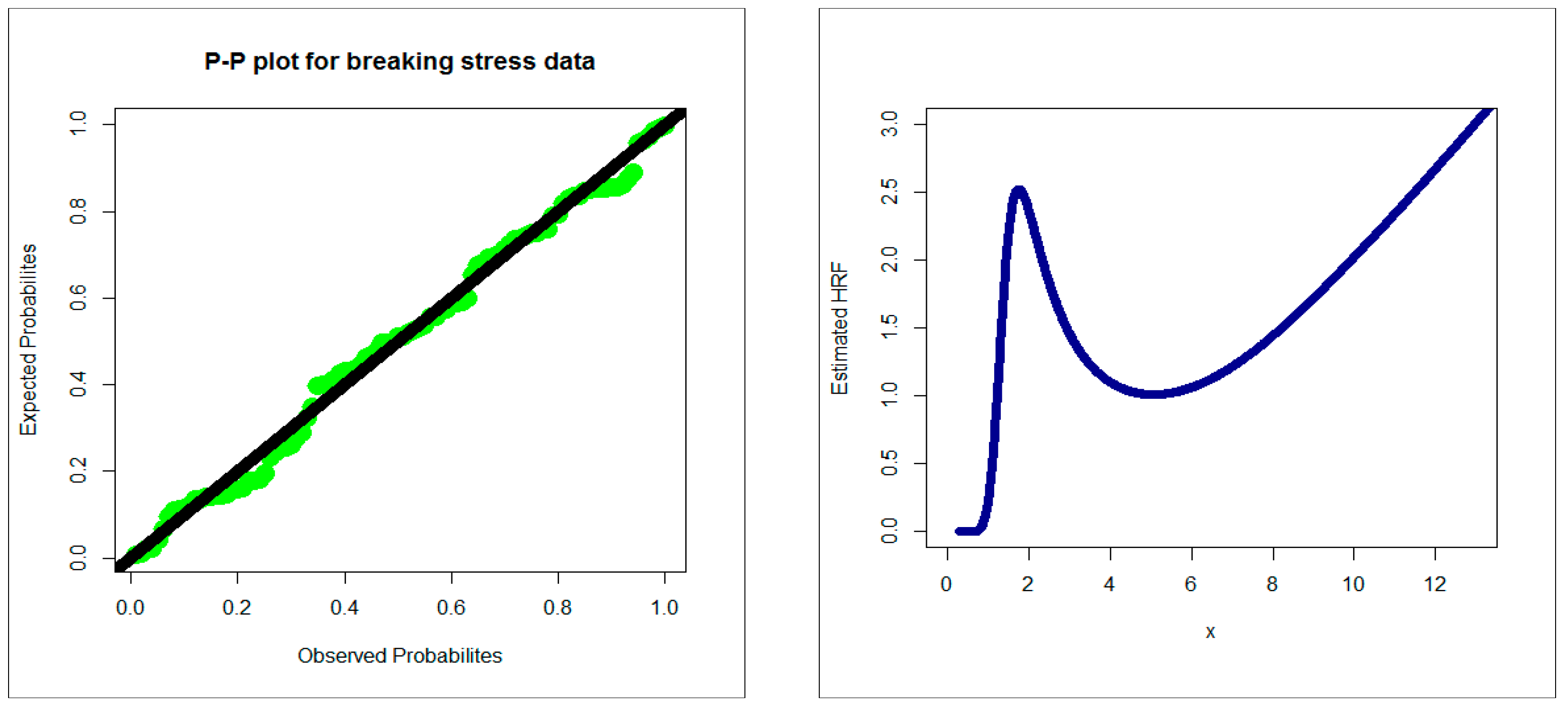
4.1. Comparing the Competitive Extensions under the Stress Data

A total of 100 observations on the breaking stress of carbon fibers make up the first uncensored data set (see Nichols and Padgett [10]). Figure 1 shows the NKDE panel (the first row, left panel), the TTT panel (the first row, right panel), the box panel (the second row, left panel), the Q-Q panel (the second row, right panel), scattergram panel (the third row, left panel), and the skewness-kurtosis panel (the third row, right panel). The breaking stress of carbon fibers is shown in Figure 1 (first-row left panel) to be the asymmetric bimodal and heavy right tail. It is evident from Figure 1’s panel in the first row to the right that the HRF for the current data is monotonically rising. It can be seen from Figure 1’s second-row left panel and second-row right panel that these data contain some extreme values. The current data cannot be described by theoretical distributions, such as the normal, uniform, exponential, logistic, beta, lognormal, and Weibull distributions, as seen in Figure 1’s third row right panel. The Shapiro test (ST) was performed to examine the extent to which the first data depended on a normal distribution, and the results were as ST = 0.7165, p-value = 1.33 × 10⁻¹² which means that this data set does not follow the normal distribution.

Figure 1. The NKDE panel (the first row, left panel), the TTT panel (the first row, right panel), the box panel (the second row, left panel), the Q-Q panel (the second row, right panel), scattergram panel (the third row, left panel), and the skewness-kurtosis panel (the third row, right panel) for the breaking stress of carbon fibers data.

The statistics Cramér–von Mises criterion (CVM), Anderson–Darling test (AD), Kolmogorov–Smirnov test (KS), and the corresponding p-values ($P_{\upsilon }$) for all fitted models are presented in Table 2. The MLEs and corresponding standard errors (SEs) are reported in Table 3. From Table 2, the GGR-RW model gives the lowest values CVM = 0.0612, AD = 0.4467, KS = 0.05887, and $P_{\upsilon }$ = 0.8789 as compared to the other models. As a result, the GGR-RW is the model that should be selected. In Figure 2, the estimated PDF and CDF are shown. For the current data, Figure 3 shows the Probability-Probability (P-P) panel and estimated HRF. We can see from Figure 2 and Figure 3 that the new GGR-RW model offers good fits for the empirical functions.

Table 2. CVM, AD, KS, and $P_{\upsilon }$ for the breaking stress of carbon fibers data.

$\mathbf{Criteria}\to$	Goodness of Fit Criteria
$\mathbf{Model}\downarrow$	AD	CVM	$\mathbf{KS} \left({\mathit{P}}_{\mathit{\upsilon }}\right)$
GGR-RW	0.44671	0.0612	0.05887 (0.8789)
OLLE-RW	0.96404	0.1204	0.5561 ($<0.0001$)
Mc-RW	1.0608	0.1333	0.0807 (0.53323)
OLLE-RR	1.2120	0.1553	0.6550 ($<0.0001$)
Beta-RW	0.6207	0.0809	0.0757 (0.61472)
Kum-RW	0.6217	0.0812	0.07596 (0.6118)
RW	0.7657	0.1090	0.08746 (0.4282)
E-RW	0.7658	0.1093	0.0875 (0.428667)
MO-RW	0.6142	0.0886	0.07629 (0.51677)
OB-RW	0.4717	0.0662	0.06310 (0.82202)
OLL-RR	1.2120	0.1553	0.6550 ($<0.0001$)
T-RW	0.6209	0.0873	0.07821 (0.573443)

Table 3. MLEs and SEs for the breaking stress of carbon fibers data.

$\mathbf{Estimates} \to$ $\mathbf{Model}\downarrow$	Estimates
	$\widehat{\mathit{a}}$	$\widehat{\mathit{b}}$	$\widehat{\mathit{c}}$	$\widehat{{\mathit{\delta }}_1}$	$\widehat{{\mathit{\delta }}_2}$
GGR-RW	250.2153 (393.532)	0.029866 (0.01752)		74.12585 (68.9231)	1.1729339 (0.222893)
GGR-RW	5.195441 (0.00123)	0.59904 (0.0323)		1.040482 (0.0444)	1.232432 (0.003323)
OLLE-RW	0.135122 (0.011223)		3.72164 (0.00343)	0.92963 (0.0034)	21.31942 (0.00363)
OLLE-RR	0.4946375 (0.04143)		0.067433 (0.71955)	1.742628 (9.30073)
OLL-RR	0.494583 (0.04139)		0.452423 (0.03877)
RW				1.39688 (0.0336)	4.37255 (0.3278)
Kum-RW		0.84892 (16.083)	1.62393 (0.6979)	1.63413 (9.0492)	3.42083 (0.7639)
E-RW		0.93951 (3.5434)		1.41693 (2.56832)	0.9391 (0.3273)
Beta-RW		0.73463 (1.5290)	1.58383 (0.7137)	1.66844 (0.7662)	3.51126 (0.9680)
T-RW	$-$0.71663 (0.26162)			1.265642 (0.0571)	4.71219 (0.36590)
MO-RW		0.003349 (0.00092)		6.23965 (1.01348)	1.241982 (0.1180)
Mc-RW	0.85035 (0.13537)	44.42332 (25.1324)	19.8591 (6.7066)	0.02039 (0.00683)	46.9745 (21.8735)

Figure 2. Estimated PDF (left right) and estimated CDF (right) for the breaking stress of carbon fibers data.

Figure 3. P-P panel (left) and estimated HRF (right) for the breaking stress of carbon fiber data.

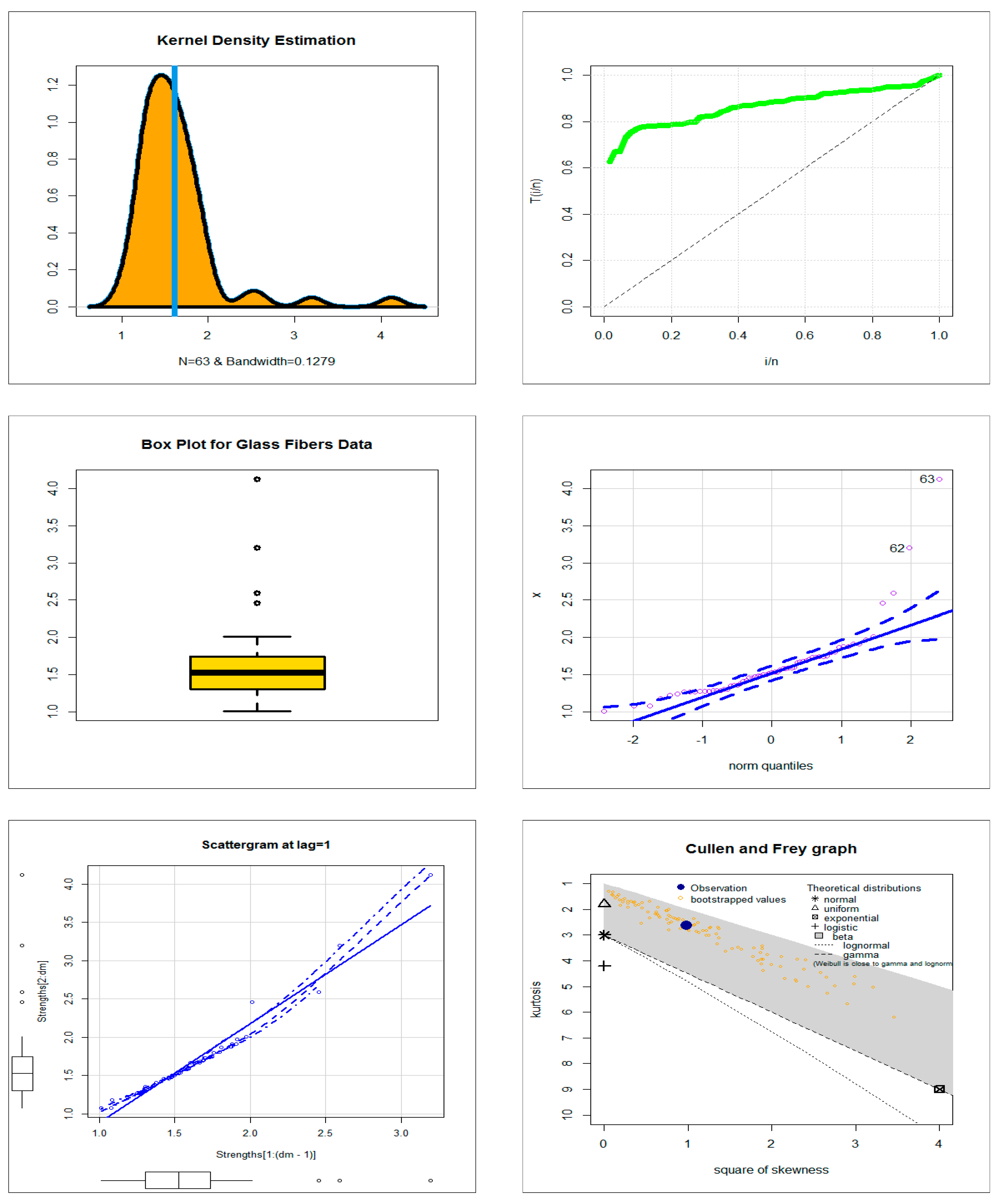
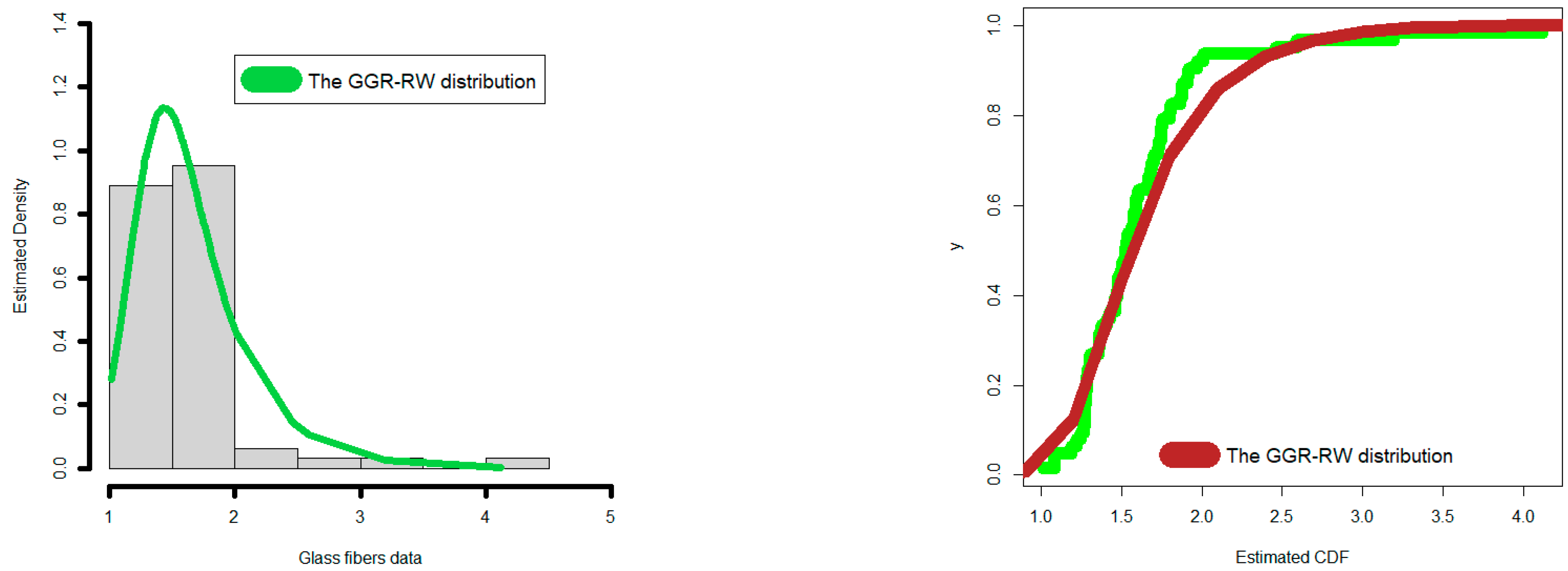
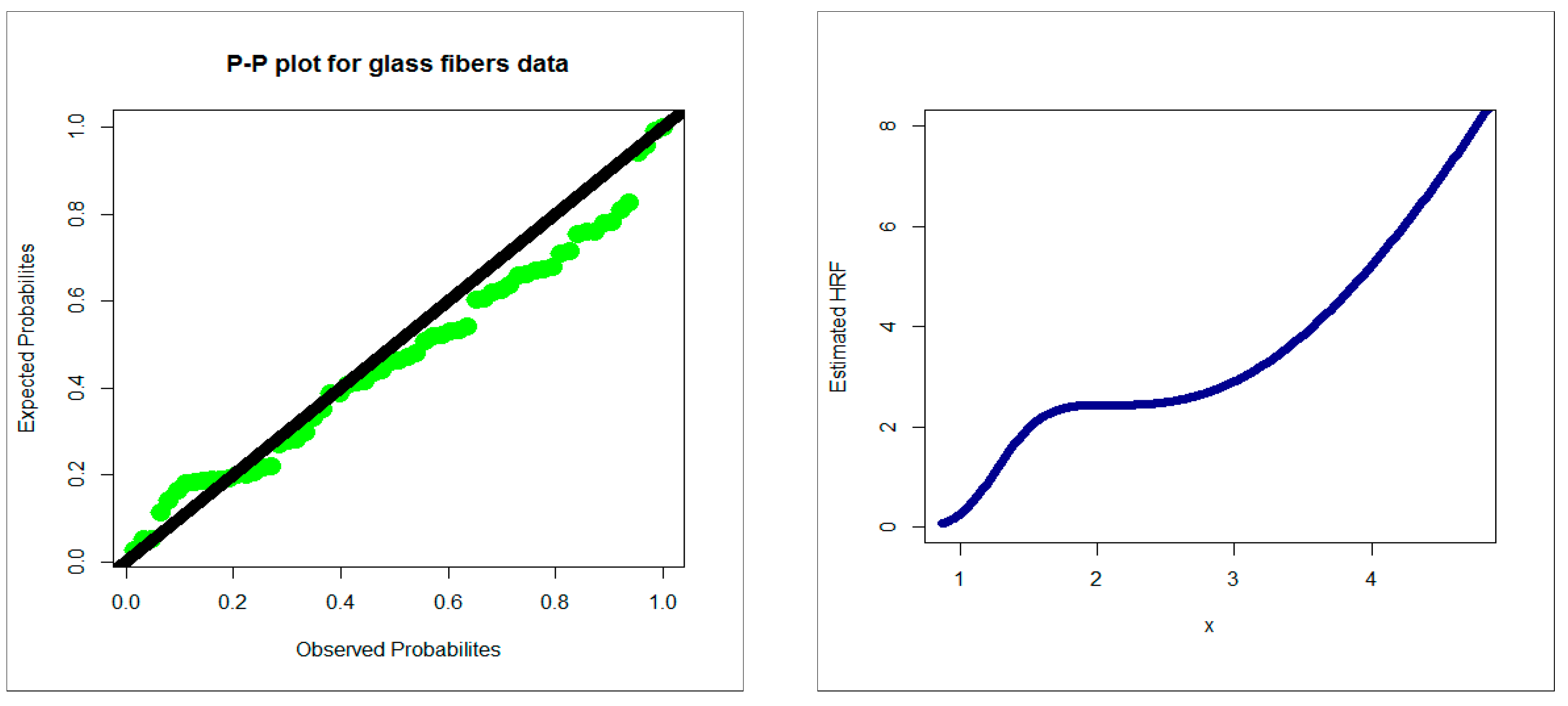
4.2. Comparing the Competitive Extensions under the Glass Fiber Data

The second data set is a list of glass fiber strengths provided by Smith and Naylor (1987) [11]. Figure 4 gives the NKDE panel (the first-row left panel), the TTT panel (the first row, right panel), the box panel (the second row, left panel), the Q-Q panel (the second row, right panel), the scattergram panel (the third row, left panel), and the skewness-kurtosis panel (the third row, right panel). Figure 4 (the first row, left panel) indicates that the glass fiber data is asymmetric bimodal and heavy right tail. Figure 4 (the first row, right panel) indicates that the HRF of the glass fiber data is monotonically increasing. The glass fiber data in Figure 4 (second-row left panel and second-row right panel) include some extreme values. Glass fiber data cannot be described by theoretical distributions, such as the normal, uniform, exponential, logistic, beta, lognormal, and Weibull distributions, according to Figure 4’s third-row right panel. The ST was performed to examine the extent to which the second data depended on a normal distribution. The results were as ST = 0.72409, p-value = 1.443 × 10⁻⁹, which means that this data set does not follow the normal distribution.

Figure 4. The NKDE panel (the first row, left panel), the TTT panel (the first row, right panel), the box panel (the second row, left panel), the Q-Q panel (the second row, right panel), scattergram panel (the third row, left panel), and the skewness-kurtosis panel (the third row, right panel) for the glass fibers data.

Table 4 lists the statistics of CVM, AD, KS, and $P_{\upsilon }$ for each fitted model. Table 5 lists the MLEs and related SEs. In comparison to other models, the GGR-RW model provides the lowest values, CVM = 0.11304, AD = 0.89752, KS = 0.12348, and $P_{\upsilon }$ = 0.2691 (Table 4). The GGR-RW distribution can be selected as the best model as a result. In Figure 5, the estimated PDF and CDF are shown. The P-P panel and estimated HRF for the data on glass fiber are shown in Figure 6. It is evident from Figure 5 and Figure 6 that the GGR-RW model adequately fits the empirical distribution functions.

Table 4. CVM, AD, KS and $P_{\upsilon }$ for the glass fiber data.

$\mathbf{Criteria}\to$ $\mathbf{Model}\downarrow$	Goodness of Fit Criteria
	AD	CVM	$\mathbf{KS} \left({\mathit{P}}_{\mathit{\upsilon }}\right)$
GGR-RW	0.89752	0.11304	0.12348 (0.269121)
OLLE-RR	1.14697	0.15025	0.67949 ($<0.0005$)
OLLE-RW	0.83253	0.10487	0.55196 ($<0.0005$)
OLL-RR	1.14697	0.15023	0.67951 ($<0.0005$)

Table 5. MLEs and SEs for the glass fibers data.

$\mathbf{Estimates} \to$ $\mathbf{Model}\downarrow$	Estimates
	$\widehat{\mathit{a}}$	$\widehat{\mathit{b}}$	$\widehat{\mathit{c}}$	$\widehat{{\mathit{\delta }}_1}$	$\widehat{{\mathit{\delta }}_2}$
GGR-RW	14.89942 (6.22644)	0.005742 (0.00093)		53.55753 (11.9332)	1.594772 (0.09712)
OLLE-RW	0.144922 (0.01294)		0.008792 (0.00021)	1.299724 (0.00006)	24.87832 (0.00025)
OLLE-RR	0.502541 (0.05292)		0.071613 (1.13065)	1.704832 (13.4744)
OLL-RR	0.502512 0.052946		0.4559913 0.0486522

Figure 5. Estimated PDF (left) and CDF (right) for the glass fibers data.

Figure 6. P-P panel (left) and estimated HRF (right) for the glass fibers data.

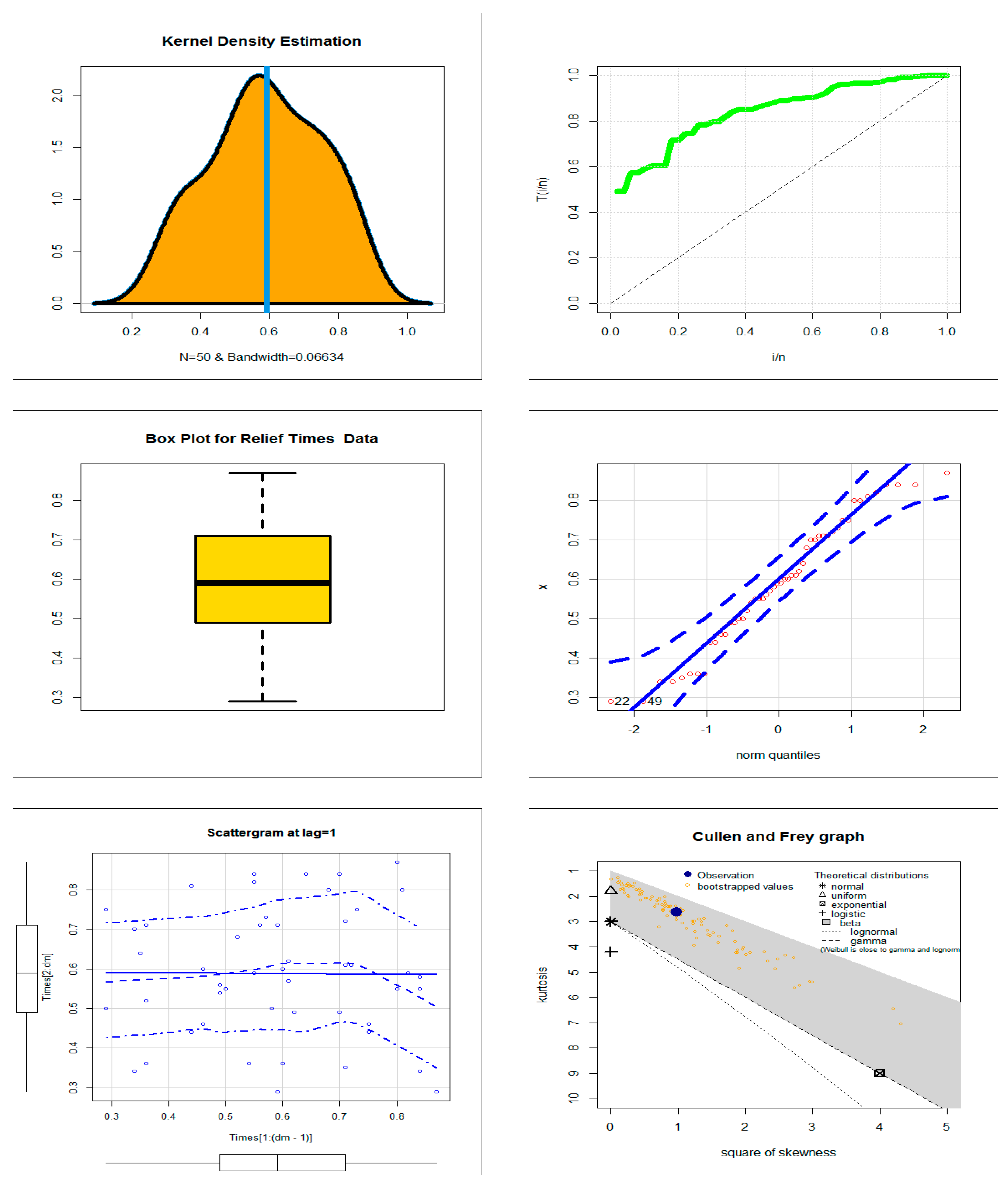
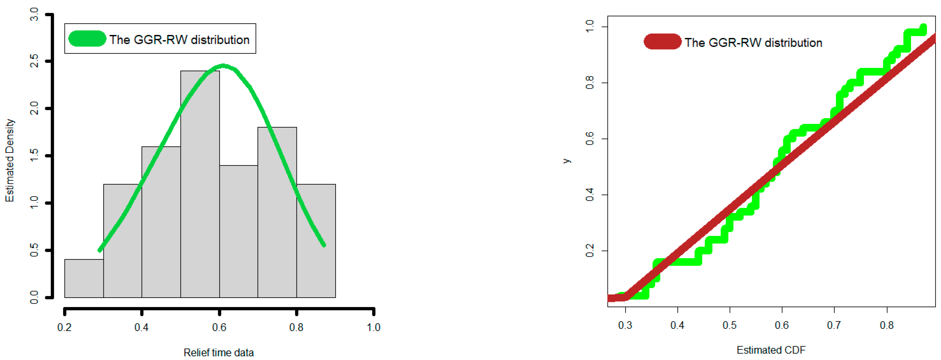
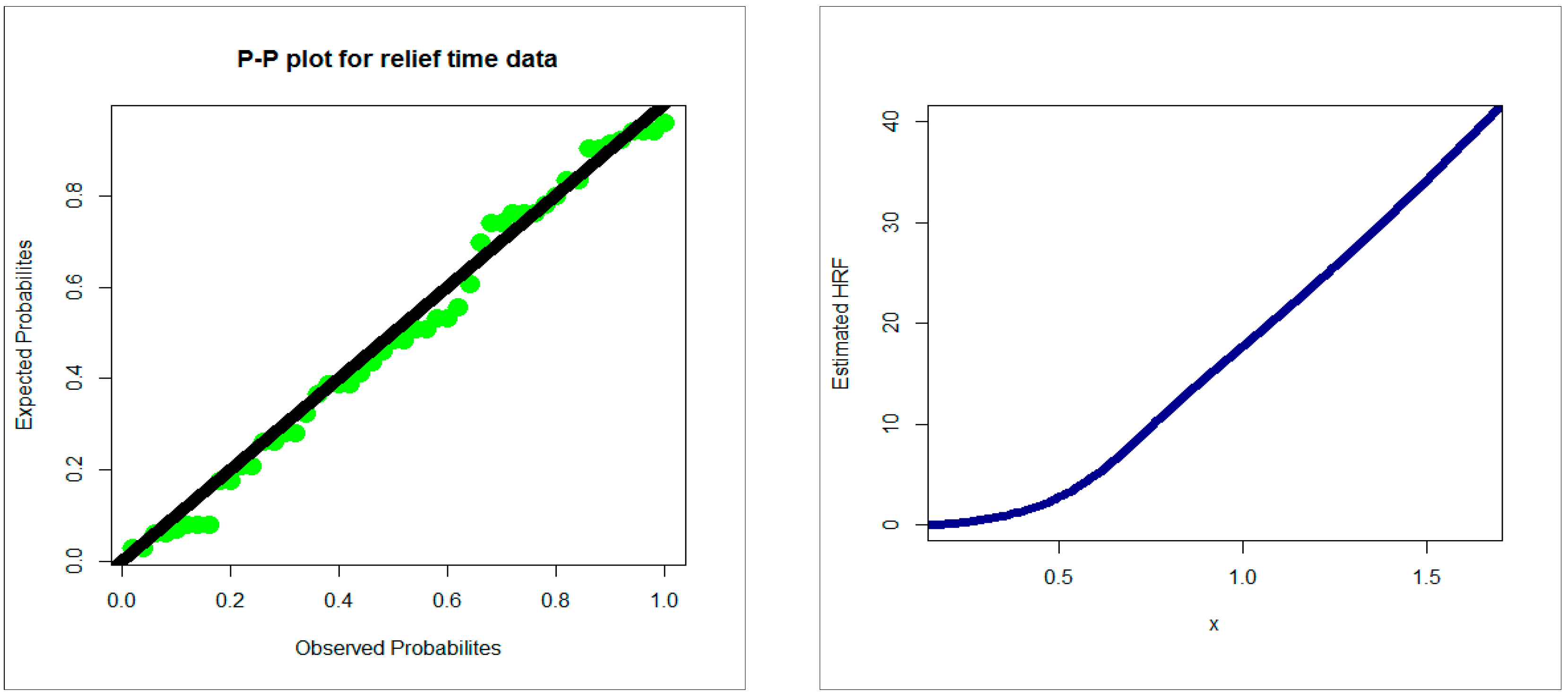
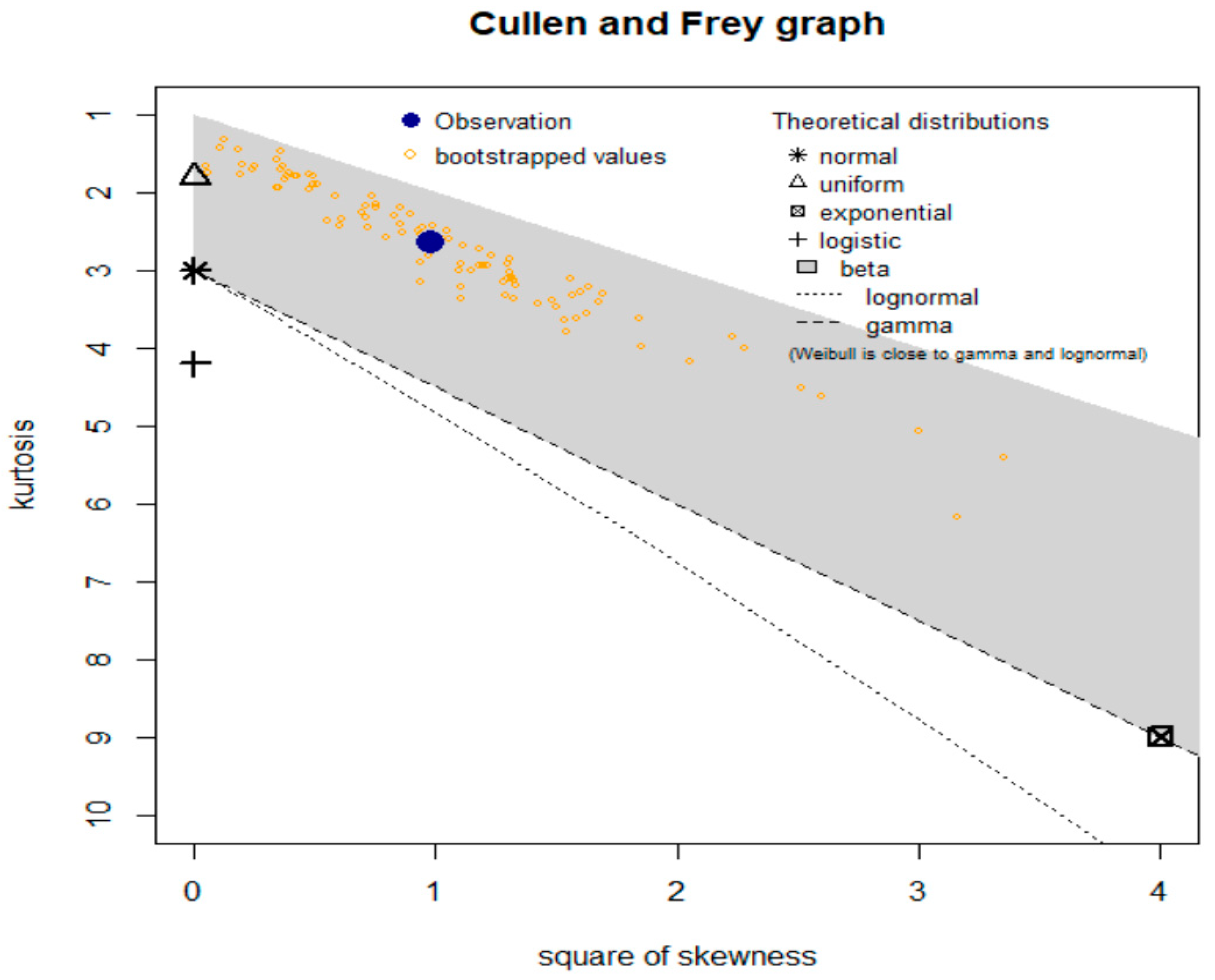
4.3. Comparing the Competitive Extensions under the Relief Times Data

The third data collection, dubbed “Wingo data”, contains all of the results from a clinical trial that measured the number of hours of pain alleviation for 50 individuals with arthritis. Figure 7 gives the NKDE panel (the first row, left panel), the TTT panel (the first row, right panel), the box panel (the second row, left panel), the Q-Q panel (the second row, right panel), the scattergram panel (the third row, left panel), and the skewness-kurtosis panel (the third row, right panel). Figure 7 (the first row, left panel) indicates that the relief time data can be considered as symmetric data. Based on Figure 7 (the first row, right panel), it is noted that the HRF of these data is monotonically increasing. Based on Figure 1 (the second row, left panel, and the second row, right panel), the relief times do not include any extreme values. It can be seen from Figure 7’s third row right panel those theoretical distributions, such as the normal, uniform, exponential, logistic, beta, lognormal, and Weibull distributions cannot explain the relief timings. The ST was performed to examine the extent to which the third data depended on a normal distribution, and the results were as ST = 0.96451 and p-value = 0.1373 which means that this data sets follow the normal distribution. However, the new presented GGR-RW model performs better than the normal distribution in modeling this data.

Figure 7. The NKDE panel (the first row, left panel), the TTT panel (the first row, right panel), the box panel (the second row, left panel), the Q-Q panel (the second row, right panel), scattergram panel (the third row, left panel), and the skewness-kurtosis panel (the third row, right panel) for the relief times.

Table 6 lists the statistics CVM, AD, KS, and $P_{\upsilon }$ for each fitted model. Table 7 lists the MLEs and related SEs. The lowest values from Table 6 for the GGR-RW model are CVM = 0.0485, AD = 0.4014, KS = 0.081911, and $P_{\upsilon }$ = 0.8906. As a result, the GGR-RW may be selected as the ideal model. Both the calculated PDF and CDF are shown in Figure 8. The P-P panel and estimated HRF for the relief periods data are shown in Figure 9. We can see from Figure 8 and Figure 9 that the new GGR-RW model offers good fits for the empirical CDFs.

Table 6. CVM, AD, KS and $P_{\upsilon }$ for the relief times data.

$\mathbf{Criteria}\to$ $\mathbf{Model}\downarrow$	Goodness of Fit Criteria
	AD	CVM	$\mathbf{KS} \left({\mathit{P}}_{\mathit{\upsilon }}\right)$
GGR-RW	0.4014	0.0485	0.081911 (0.8906)
RW	2.0301	0.3233	0.150622 (0.2066)
GOLL-RR	1.3498	0.1955	0.110083 (0.5797)
OB-RW	0.4208	0.0490	0.091243 (0.7994)
OLLE-RW	1.0988	0.1577	0.53498 ($<0.0001$)
Beta-RW	2.5133	0.3613	0.143345 (0.3601)
E-RW	2.0304	0.3233	0.150619 (0.2064)
T-RW	1.81528	0.2823	0.137013 (0.3045)

Table 7. MLEs and SEs for the relief times data.

$\mathbf{Estimates} \to$ $\mathbf{Model}\downarrow$	Estimates
	$\widehat{\mathit{a}}$	$\widehat{\mathit{b}}$	$\widehat{\mathit{c}}$	$\widehat{{\mathit{\delta }}_1}$	$\widehat{{\mathit{\delta }}_2}$
GGR-RW	0.377621 (0.6077)	0.008394 (0.00151)		21.01783 (21.46851)	1.212893 (0.45608)
OB-RW	17.79132 (0.00014)	6.996212 (4.03633)		0.126862 (0.00023)	0.178433 (0.00044)
GOLL-RR	1.961322 (0.23402)	0.111237 (0.00146)		1.412323 (0.00534)
OLLE-RW	0.066923 (0.00762)		0.00464 (0.0028)	0.35583 (0.0047)	32.5611 (0.0063)
RW				0.485933 (0.02272)	3.20785 (0.3263)
E-RW			0.90474 (18.7863)	0.50134 (3.24444)	3.20774 (0.3265)
Beta-RW		4.01545 (0.11153)	1.334933 (0.1476)	2.00223 (0.32134)	0.87017 (0.00333)
T-RW	$-$0.58161 (0.27873)			0.440232 (0.0293)	3.49742 (0.3527)

Figure 8. Estimated PDF (left) and estimated CDF (right) for the relief times.

Figure 9. P-P panel (left) and estimated HRF (right) for the relief times.

5. Risk Analysis

In this section, we will present a wide range of practical results, whether in the field of actuarial modeling or in the field of insurance applications. First, we introduce synthetic experiments to analyze actuarial risk. Secondly, we will conduct a comprehensive process study on insurance claims data.

5.1. Artificial Risk Analysis

For risk analysis and evaluation, the maximum likelihood estimation (MLE), weighted least squares estimation (WLSQ), ordinary least squares estimation (OLSQ), and Cramér-von Mises estimation (CVME) methods are considered. We will ignore the algebraic derivations and theoretical results of these methods since it is already present in a lot of statistical literature. On the other hand, we will focus a lot on the practical results and statistical applications of mathematical modeling in general and of the risk disclosure, analysis risk, and evaluation of actuarial risks. For computing the above-mentioned KRIs, the following estimation techniques are discussed in these sections: the MLE, OLSQ, WLSQ and CVME methods. Seven CLs (q = 50%, 60%, 70%, 80%, 90%, 95%, 99% and 99%) and N = 1000 with Various sample sizes (n = 20, 50, 100) are considered under ${\alpha }_0=2,b=0.5, {\delta }_1=0.7, {\delta }_2=0.3$. All results are reported in Table 8, Table 9 and Table 10. Table 8 shows the KRIs for the GGR-RW under artificial data where n = 20. Table 9 gives the KRIs for the GGR-RW under artificial data where n = 50. Table 10 lists the KRIs for the GGR-RW under artificial data where n = 100. The simulation’s primary objective is to evaluate the efficacy of the five risk analysis methodologies and select the most appropriate and efficient ones. Table 8, Table 9 and Table 10 allow us to display the significant results:

Table 8. The KRIs for the GRR-RW under artificial data where n = 20.

		$\mathbf{VAR} \left(\mathit{Y};\underset{¯}{\mathit{\varphi }}\right)$	$\mathbf{TVAR} \left(\mathit{Y};\underset{¯}{\mathit{\varphi }}\right)$	$\mathbf{TV} \left(\mathit{Y};\underset{¯}{\mathit{\varphi }}\right)$	$\mathbf{TMV} \left(\mathit{Y};\underset{¯}{\mathit{\varphi }}\right)$	$\mathbf{EL} \left(\mathit{Y};\underset{¯}{\mathit{\varphi }}\right)$
MLE	$50\%$	0.0381111	0.1486531	0.0233400	0.1603231	0.1105419
	$60\%$	0.0541547	0.1744053	0.0258538	0.1873322	0.1202507
	$70\%$	0.0782740	0.2107700	0.0291661	0.225353	0.1324959
	$80\%$	0.1189146	0.2678643	0.033902	0.2848153	0.1489497
	$90\%$	0.2057473	0.3801243	0.0419915	0.4011201	0.174377
	$95\%$	0.3123655	0.5088242	0.0499369	0.5337926	0.1964587
	$99\%$	0.6217416	0.8601832	0.0678638	0.8941151	0.2384416
LS	$50\%$	0.0374667	0.1490600	0.0241590	0.1611395	0.1115933
	$60\%$	0.0535004	0.1750774	0.0268089	0.1884819	0.121577
	$70\%$	0.0776905	0.2118756	0.0303126	0.2270319	0.1341851
	$80\%$	0.1185895	0.2697621	0.0353475	0.2874358	0.1511726
	$90\%$	0.2063194	0.3838971	0.0440212	0.4059077	0.1775778
	$95\%$	0.3144706	0.5151746	0.0526295	0.5414893	0.200704
	$99\%$	0.6301761	0.8753958	0.0723317	0.9115617	0.2452197
WLS	$50\%$	0.0342739	0.1376783	0.0210272	0.1481916	0.1034040
	$60\%$	0.0489822	0.1618043	0.0233691	0.1734889	0.1128222
	$70\%$	0.0712356	0.1959845	0.026472	0.2092206	0.1247489
	$80\%$	0.1090019	0.2498647	0.0309402	0.2653348	0.1408628
	$90\%$	0.1904255	0.3563898	0.0386510	0.3757153	0.1659643
	$95\%$	0.2912627	0.4792157	0.0463079	0.5023696	0.187953
	$99\%$	0.5868431	0.8170242	0.0638199	0.8489342	0.2301812
CVM	$50\%$	0.0373757	0.1483838	0.0239460	0.1603568	0.1110082
	$60\%$	0.0532972	0.1742681	0.0265773	0.1875568	0.1209709
	$70\%$	0.077324	0.2108897	0.0300559	0.2259176	0.1335657
	$80\%$	0.1179792	0.2685231	0.0350509	0.2860486	0.1505439
	$90\%$	0.2053027	0.3822116	0.0436372	0.4040302	0.176909
	$95\%$	0.3130633	0.5129930	0.0521284	0.5390572	0.1999297
	$99\%$	0.6276448	0.8716274	0.0714515	0.9073532	0.2439827

Table 9. The KRIs for the GRR-RW under artificial data where n = 50.

		$\mathbf{VAR} \left(\mathit{Y};\underset{¯}{\mathit{\varphi }}\right)$	$\mathbf{TVAR} \left(\mathit{Y};\underset{¯}{\mathit{\varphi }}\right)$	$\mathbf{TV} \left(\mathit{Y};\underset{¯}{\mathit{\varphi }}\right)$	$\mathbf{TMV} \left(\mathit{Y};\underset{¯}{\mathit{\varphi }}\right)$	$\mathbf{EL} \left(\mathit{Y};\underset{¯}{\mathit{\varphi }}\right)$
MLE	$50\%$	0.0373339	0.1457556	0.0222846	0.1568979	0.1084217
	$60\%$	0.053175	0.1710013	0.0246639	0.1833332	0.1178263
	$70\%$	0.0769553	0.2066087	0.027798	0.2205076	0.1296533
	$80\%$	0.1169123	0.2624301	0.0322832	0.2785717	0.1455178
	$90\%$	0.2019247	0.371995	0.0399747	0.3919824	0.1700704
	$95\%$	0.3059526	0.497478	0.0475827	0.5212694	0.1915254
	$99\%$	0.6074063	0.8402381	0.0649493	0.8727127	0.2328318
LS	$50\%$	0.0368937	0.1454241	0.0225629	0.1567055	0.1085304
	$60\%$	0.0526345	0.1707094	0.0250017	0.1832103	0.1180749
	$70\%$	0.0763185	0.2064162	0.0282203	0.2205263	0.1300977
	$80\%$	0.1162205	0.2624769	0.0328365	0.2788952	0.1462565
	$90\%$	0.2014086	0.3727327	0.0407754	0.3931204	0.1713242
	$95\%$	0.3059839	0.4992581	0.0486494	0.5235828	0.1932743
	$99\%$	0.6100726	0.8456811	0.0666786	0.8790204	0.2356086
WLS	$50\%$	0.0364107	0.1431778	0.0217920	0.1540738	0.1067671
	$60\%$	0.0519162	0.1680499	0.0241419	0.1801208	0.1161336
	$70\%$	0.0752356	0.2031654	0.0272418	0.2167863	0.1279298
	$80\%$	0.1145055	0.2582839	0.0316851	0.2741264	0.1437783
	$90\%$	0.1982991	0.3666467	0.0393191	0.3863063	0.1683476
	$95\%$	0.3011073	0.4909484	0.0468821	0.5143894	0.189841
	$99\%$	0.5998334	0.8310739	0.064172	0.8631599	0.2312405
CVM	$50\%$	0.0371846	0.1459834	0.0225801	0.1572735	0.1087988
	$60\%$	0.0530105	0.1713256	0.0250089	0.1838300	0.1183151
	$70\%$	0.0768006	0.2070954	0.0282116	0.2212012	0.1302948
	$80\%$	0.116839	0.2632221	0.0328008	0.2796225	0.1463831
	$90\%$	0.2022038	0.3735195	0.0406832	0.3938610	0.1713156
	$95\%$	0.3068647	0.4999904	0.0484911	0.5242360	0.1931258
	$99\%$	0.6107723	0.8459199	0.0663415	0.8790906	0.2351476

Table 10. The KRIs for the GRR-RW under artificial data where n = 100.

		$\mathbf{VAR} \left(\mathit{Y};\underset{¯}{\mathit{\varphi }}\right)$	$\mathbf{TVAR} \left(\mathit{Y};\underset{¯}{\mathit{\varphi }}\right)$	$\mathbf{TV} \left(\mathit{Y};\underset{¯}{\mathit{\varphi }}\right)$	$\mathbf{TMV} \left(\mathit{Y};\underset{¯}{\mathit{\varphi }}\right)$	$\mathbf{EL} \left(\mathit{Y};\underset{¯}{\mathit{\varphi }}\right)$
MLE	$50\%$	0.0370309	0.14445380	0.02182030	0.155364	0.1074229
	60%	0.0527590	0.1694630	0.0241430	0.1815345	0.1167039
	$70\%$	0.0763570	0.2047240	0.0272020	0.2183249	0.128367
	$80\%$	0.1159737	0.2599773	0.0315796	0.2757671	0.1440036
	$90\%$	0.2001615	0.3683678	0.0390906	0.3879131	0.1682064
	$95\%$	0.3030780	0.492457	0.0465288	0.5157214	0.189379
	$99\%$	0.6011336	0.8313712	0.0635422	0.8631423	0.2302376
LS	$50\%$	0.0368989	0.1445928	0.0220315	0.1556085	0.1076939
	$60\%$	0.0526166	0.1696712	0.0243896	0.1818660	0.1170547
	$70\%$	0.0762228	0.2050486	0.0274979	0.2187975	0.1288258
	$80\%$	0.1158991	0.2605198	0.0319508	0.2764952	0.1446207
	$90\%$	0.2003359	0.3694332	0.0396026	0.3892345	0.1690973
	$95\%$	0.3036975	0.4942325	0.0471918	0.5178284	0.1905351
	$99\%$	0.6035121	0.8354713	0.0645834	0.867763	0.2319592
WLS	$50\%$	0.0373859	0.1456207	0.0221189	0.1566801	0.1082348
	$60\%$	0.0532489	0.1708169	0.0244691	0.1830515	0.117568
	$70\%$	0.0770415	0.2063356	0.0275636	0.2201174	0.1292942
	$80\%$	0.1169704	0.2619815	0.0319904	0.2779767	0.1450112
	$90\%$	0.2017831	0.3711118	0.0395819	0.3909027	0.1693287
	$95\%$	0.3054192	0.4960116	0.0470956	0.5195594	0.1905925
	$99\%$	0.6054054	0.8370118	0.0642700	0.8691468	0.2316064
CVM	$50\%$	0.0370433	0.1448759	0.0220367	0.1558943	0.1078326
	$60\%$	0.0528079	0.1699834	0.0243888	0.1821778	0.1171755
	$70\%$	0.0764724	0.2053916	0.027488	0.2191356	0.1289192
	$80\%$	0.1162215	0.2608921	0.0319261	0.2768551	0.1446705
	$90\%$	0.2007439	0.3698128	0.0395488	0.3895872	0.1690689
	$95\%$	0.3041334	0.4945666	0.0471064	0.5181198	0.1904333
	$99\%$	0.6038073	0.8355222	0.0644203	0.8677323	0.2317149

• The $\mathrm{VAR}$($Y;\widehat{\underset{\_}{\mathit{\varphi }}}$), $\mathrm{TVAR}\left(Y;\widehat{\underset{\_}{\mathit{\varphi }}}\right)$ and $\mathrm{TMV}\left(Y;\widehat{\underset{\_}{\mathit{\varphi }}}\right)$ increase when q increases for all estimation methods.
• The $\mathrm{TV}\left(Y;\widehat{\underset{\_}{\mathit{\varphi }}}\right)$ and $\mathrm{EL}\left(Y;\widehat{\underset{\_}{\mathit{\varphi }}}\right)$ decrease when q increases for all estimation methods.
• The three tables’ results enable us to verify that all approaches are valid and that it is impossible to categorically recommend one approach over another. Given this fundamental finding, we are obliged to develop an application based on real data in the hopes that it would enable us to select one strategy over another and identify the best and most appropriate methods. In other words, even though the results from the five ways to risk assessment were equivalent, the simulation research did not help us decide how to balance the methodologies. These convergent findings comfort us that, when modelling actuarial data and evaluating risk, all methodologies function satisfactorily and within allowable limits.

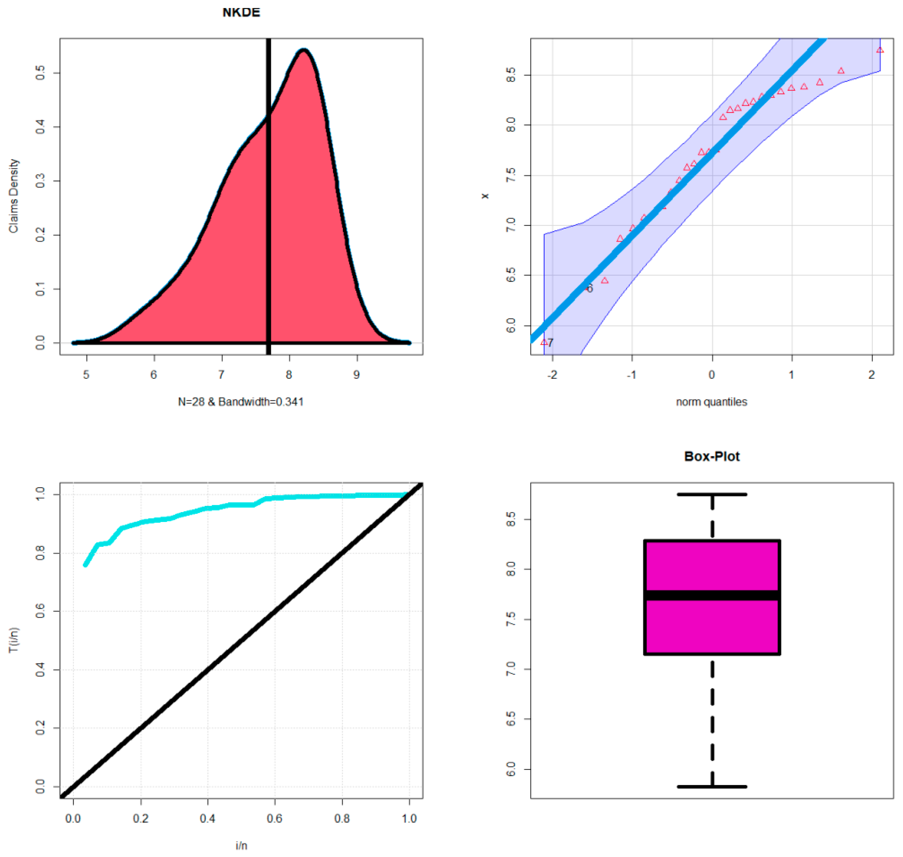
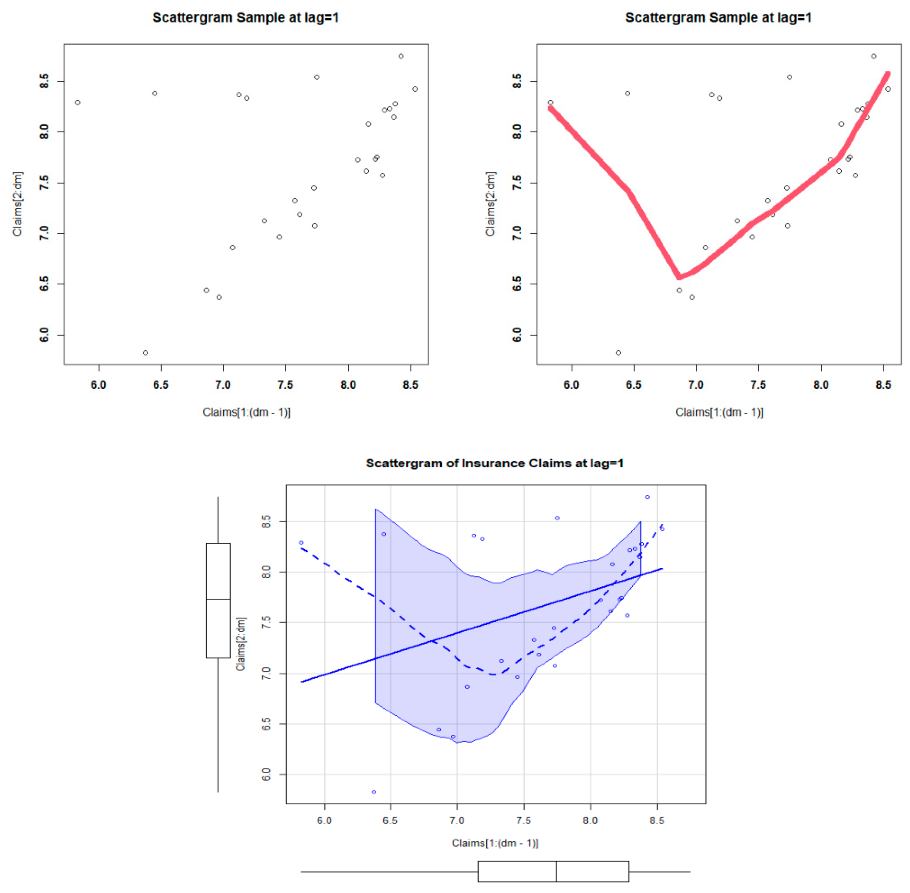
5.2. Insurance Data for Risk Analysis

The temporal growth of claims over time for each pertinent exposure (or origin) period is typically represented in the chronological insurance real data as a triangle. The year the insurance policy was purchased or the time period during which the loss happened can be considered the exposure period. The origin period need not be annual, as it should be obvious. Origin periods, for instance, might be monthly or quarterly. The length of time it takes for an origin period to develop is referred to as the claim age or claim lag. Data from various insurances are frequently combined to indicate consistent company lines, division levels, or risks. For the purposes of this study, we use a U.K. Motor Non-Comprehensive account as an illustration of the insurance claims payment triangle. We choose to set the origin period between 2007 and 2013 for practical reasons (see Mohamed et al. [12] and Hamed et al. [13]). The insurance claims payment data frame displays the claims data in a manner similar to how a database would normally keep it. The development year, incremental payments, and origin year are all listed in the first column and range from 2007 to 2013. It is crucial to keep in mind that this data on insurance claims were initially examined using a probability-based distribution. The analysis of real data can be carried out numerically, visually, or by combining the two. The numerical method, as well as a few graphical tools, such as the skewness-kurtosis panel (or the Cullen and Frey panel), are taken into consideration when assessing initial fits of theoretical distributions such as the normal, uniform, exponential, logistic, beta, lognormal, and Weibull (see Figure 9).

Our negatively skewed actuarial data, with a kurtosis of less than three, are shown in Figure 10. The NKDE method is used to examine the initial shape of the insurance claims density (see Figure 11, top left panel), and the P-P panel is used to assess the “normality” of the current data (see Figure 11, top right panel), the TTT panel is used to assess the initial shape of the empirical HRF (see Figure 11, bottom left panel), and the “box panel” is used to identify the explanatory variables (see Figure 10, the bottom right panel). Figure 11 shows the initial density as an asymmetric function with a left tail (top left panel). Figure 11 does not support any irrational claims (bottom right panel). According to Figure 11’s bottom left panel, the HRF for the models that explain the current data should similarly be monotonically expanding. Figure 12 displays the scattergrams for the data on insurance claims. Figure 13 (left panel) displays the autocorrelation function (ACF) for the data on insurance claims, and Figure 13 (right panel) displays the partial autocorrelation function (partial ACF).

Figure 10. Cullen-Frey panel for the actuarial claims data.

Figure 11. NKDE (top left), Q-Q (top right), TTT (bottom left), and box panels (bottom right) for the claims data.

Figure 12. The scattergrams.

Figure 13. The ACF (left) and the partial ACF (right) for the insurance claims data.

We offer the ACF to show how the correlation between any two signal values changes as a function of the distance between them. The theoretical ACF provides no information about the process’s frequency content; instead, it measures the stochastic process memory in the time domain. Figure 13 illustrates how hills and valleys are distributed across the surface when Lag = k = 1 (the left panel). The theoretical partial ACF with Lag = k = 1 is also presented; see Figure 13 (the right panel). The initial lag value is demonstrated in Figure 13 (the right panel) to be statistically significant, in contrast to the other partial autocorrelations for all other lags. The first NKDE exhibits an asymmetric density with a left tail, as shown in Figure 11’s top left panel. On the other hand, the novel model’s interview, matching, and density are important in statistical modeling since they take into account the left tail shape. Therefore, it is recommended to simulate insurance claim payouts using the GGR-RW model. We present an application for risk analysis under VAR, TVAR, TV, TMV, and $\mathrm{EL} \mathrm{that} \mathrm{measures}$ insurance claims data. The risk analysis is performed for some confidence levels as follows:

$$q=50\%,60\%,70\%,80\%,90\%,95\%,99\% \mathrm{and} 99\%.$$

The GGR-RW and RW models estimate the five metrics. The KRIs for the GGR-RW under insurance claims data are shown in Table 11. The estimators and ranks for the GGR-RW model under the claims data are shown in Table 12 for all estimations. The KRIs for the GGR-RW are listed in Table 13 under statistics on insurance claims. The estimators and ranks for the RW model under the claims data are shown in Table 14 for all estimations. The estimators and rankings for each estimating method are shown in the table for the RW model under the claims data. Because it is the foundational distribution upon which the new distribution is based, the RW distribution was chosen. These tables’ conclusions are summarized as follows:

Table 11. The KRIs for the GRR-RW under insurance claims data.

		$\mathbf{VAR} \left(\mathit{Y};\underset{¯}{\mathit{\varphi }}\right)$	$\mathbf{TVAR} \left(\mathit{Y};\underset{¯}{\mathit{\varphi }}\right)$	$\mathbf{TV} \left(\mathit{Y};\underset{¯}{\mathit{\varphi }}\right)$	$\mathbf{TMV} \left(\mathit{Y};\underset{¯}{\mathit{\varphi }}\right)$	$\mathbf{EL} \left(\mathit{Y};\underset{¯}{\mathit{\varphi }}\right)$
MLE	$50\%$	2519.589871	4267.691033	3,540,150.406026	1,774,342.894046	1748.101162
	$60\%$	2925.721995	4653.938764	3,669,072.521249	1,839,190.199388	1728.216769
	$70\%$	3413.601872	5152.008492	3,909,892.629211	1,960,098.323098	1738.40662
	$80\%$	4075.783589	5868.385465	4,288,227.900333	2,149,982.335632	1792.601877
	$90\%$	5218.837237	7158.545734	4,934,867.46325	2,474,592.277359	1939.708497
	$95\%$	6438.143819	8557.764414	6,119,681.689183	3,068,398.609005	2119.620595
	$99\%$	9747.670085	12,352.578196	8,779,151.168388	4,401,928.162391	2604.908111
OLSQ	$50\%$	2428.50708	4865.81245	9,023,336.47326	4,516,534.04908	2437.30537
	$60\%$	2932.40857	5433.64085	9,547,186.93457	4,779,027.10814	2501.23228
	$70\%$	3564.63797	6167.11262	11,189,826.32321	5,601,080.27423	2602.47465
	$80\%$	4465.10947	7244.54736	12,380,274.28873	6,197,381.69173	2779.4379
	$90\%$	6120.70566	9336.0422	16,098,692.10948	8,058,682.09694	3215.33654
	$95\%$	8009.94191	11,695.34684	21,542,109.96081	10,782,750.32724	3685.40493
	$99\%$	13,665.84114	18,627.28911	36,958,017.28968	18,497,635.93395	4961.44797
WLSQ	$50\%$	2356.17122	4108.2022	3,439,375.14482	1,723,795.77462	1752.03099
	$60\%$	2767.2538	4495.98899	3,543,850.04098	1,776,421.00948	1728.73519
	$70\%$	3260.32173	4993.20737	3,729,494.08495	1,869,740.24984	1732.88564
	$80\%$	3927.39086	5703.45655	4,062,565.44978	2,036,986.18143	1776.06568
	$90\%$	5071.69421	6976.10477	4,779,635.04769	2,396,793.62862	1904.41056
	$95\%$	6281.71599	8352.06028	5,653,941.85453	2,835,322.98755	2070.34429
	$99\%$	9514.1782	12,042.68509	8,239,930.80908	4,132,008.08963	2528.50689
CVME	$50\%$	2440.48715	4680.62835	6,934,737.28581	3,472,049.27125	2240.1412
	$60\%$	2918.03280	5186.36109	7,534,972.10069	3,772,672.41143	2268.32829
	$70\%$	3510.16653	5847.41837	8,012,409.48002	4,012,052.15838	2337.25184
	$80\%$	4342.45308	6818.48345	9,433,643.36101	4,723,640.16395	2476.03037
	$90\%$	5846.10485	8654.84099	12,514,954.3509	6,266,132.01648	2808.73614
	$95\%$	7529.80733	10,735.92128	16,138,733.3737	8,080,102.60813	3206.11394
	$99\%$	12,431.2469	16,642.80352	25,779,255.9529	12,906,270.7800	4211.55663

Table 12. The estimations for all estimation methods under the GRR-RW model.

Methods	$\widehat{\mathit{a}}$	$\widehat{\mathit{b}}$	$\widehat{{\mathit{\delta }}_1}$	$\widehat{{\mathit{\delta }}_2}$
MLE	0.00109	0.43439	2.71691	0.16504
LS	0.00065	0.32104	2.54461	0.12257
WLS	0.00459	0.76214	2.04483	0.18936
CVM	0.00084	0.37663	2.39879	0.13348

Table 13. The KRIs for the RW under insurance claims data.

		$\mathbf{VAR} \left(\mathit{Y};\widehat{{\mathit{\delta }}_1},\widehat{{\mathit{\delta }}_2}\right)$	$\mathbf{TVR} \left(\mathit{Y};\widehat{{\mathit{\delta }}_1},\widehat{{\mathit{\delta }}_2}\right)$	$\mathbf{TV} \left(\mathit{Y};\widehat{{\mathit{\delta }}_1},\widehat{{\mathit{\delta }}_2}\right)$	$\mathbf{TMV} \left(\mathit{Y};\widehat{{\mathit{\delta }}_1},\widehat{{\mathit{\delta }}_2}\right)$	$\mathbf{EL} \left(\mathit{Y};\widehat{{\mathit{\delta }}_1},\widehat{{\mathit{\delta }}_2}\right)$
MLE	$50\%$	1986.487789	11,961.555933	174,419,897,519.9525	87,209,960,721.53221	9975.068144
	$60\%$	2536.462153	14,390.782535	217,997,610,644.2704	108,998,819,712.9177	11,854.320382
	$70\%$	3381.788446	18,212.884768	290,611,198,248.8563	145,305,617,337.3129	14,831.096322
	$80\%$	4923.241114	25,288.557461	435,793,880,982.5539	217,896,965,779.8344	20,365.316347
	$90\%$	8978.892448	44,037.774889	870,728,145,024.2504	435,364,116,549.9001	35,058.882441
	$95\%$	15,979.12723	76,311.911159	1,739,359,709,696.955	869,679,931,160.3890	60,332.783923
	$99\%$	58,937.60432	270,450.59761	8,648,937,166,516.464	4,324,468,853,708.830	211,512.99328
LS	$50\%$	2226.27121	9174.03623	35,221,234,657.96799	17,610,626,503.02022	6947.76502
	$60\%$	2764.08554	10,847.551	44,014,544,061.32928	22,007,282,878.21564	8083.46547
	$70\%$	3565.72511	13,418.65557	58,664,352,289.24406	29,332,189,563.2776	9852.93045
	$80\%$	4972.24847	18,032.50003	87,948,130,492.44542	43,974,083,278.72273	13,060.25156
	$90\%$	8464.56169	29,681.73496	175,453,235,244.5421	87,726,647,304.00603	21,217.17327
	$95\%$	14,100.50824	48,626.87171	350,184,932,240.5994	175,092,514,747.1714	34,526.36347
	$99\%$	44,780.28947	151,748.59629	1,737,405,220,156.72	868,702,761,826.9589	106,968.30682
WLS	$50\%$	1964.20669	4830.43197	353,521,360.01739	176,765,510.44066	2866.22528
	$60\%$	2314.75014	5505.26712	439,620,494.28391	219,815,752.40908	3190.51699
	$70\%$	2808.25355	6491.97705	582,260,408.85219	291,136,696.40314	3683.7235
	$80\%$	3614.31526	8152.00969	865,097,200.4972	432,556,752.25829	4537.69443
	$90\%$	5412.18198	11,944.5794	1,701,168,649.8689	850,596,269.51388	6532.39742
	$95\%$	7972.02825	17,419.4644	3,341,868,718.7883	1,670,951,778.8585	9447.43615
	$99\%$	19,161.39616	41,550.35309	15,948,264,082.767	7,974,173,591.7366	22,388.9569
CVM	$50\%$	2229.99377	8126.51599	16,383,249,373.39099	8,191,632,813.21149	5896.52223
	$60\%$	2739.42855	9540.45443	20,470,957,007.79706	10,235,488,044.35295	6801.02588
	$70\%$	3489.97698	11,691.68313	27,278,563,176.74898	13,639,293,280.05762	8201.70615
	$80\%$	4787.7631	15,503.20904	40,882,367,103.10032	20,441,199,054.7592	10,715.44594
	$90\%$	7940.21618	24,938.28648	81,425,453,617.80911	40,712,751,747.19104	16,998.0703
	$95\%$	12,899.51936	39,927.04311	162,397,882,831.5135	81,198,981,342.79988	27,027.52374
	$99\%$	38,705.15155	118,195.6688	804,158,697,120.1825	402,079,466,755.7600	79,490.51725

Table 14. The estimations for all estimation methods under the RW model.

Methods	$\widehat{{\mathit{\delta }}_1}$	$\widehat{{\mathit{\delta }}_2}$
MLE	1481.24152	1.24882
LS	1716.84523	1.41054
WLS	1612.67569	1.85864
CVM	1741.81127	1.48342

• For all risk assessment methods |$q=50\%,\dots , 99\%$:

  $$\mathrm{VAR}\left(Y;\underset{\_}{\mathit{\varphi }}\right){|}_{q=50\%}<\mathrm{VAR}\left(Y;\underset{\_}{\mathit{\varphi }}\right){|}_{q=60\%}\dots <\mathrm{VAR}\left(Y;\underset{\_}{\mathit{\varphi }}\right){|}_{q=99\%}.$$
• For all risk assessment methods |$q=50\%,60\%,70\%,80\%,90\%,95\%,99\% \mathrm{and} 99\%$:

  $$\mathrm{TVAR}\left(Y;\underset{\_}{\mathit{\varphi }}\right){|}_{q=50\%}<\mathrm{TVAR}\left(Y;\underset{\_}{\mathit{\varphi }}\right){|}_{q=60\%}\dots <\mathrm{TVAR}\left(Y;\underset{\_}{\mathit{\varphi }}\right){|}_{q=99\%}.$$
• For Most risk assessment methods |$q=60\%,\dots , 99\%$:

  $$\mathrm{TV}\left(Y;\underset{\_}{\mathit{\varphi }}\right){|}_{q=50\%}<\mathrm{TV}\left(Y;\underset{\_}{\mathit{\varphi }}\right){|}_{q=60\%}\dots <\mathrm{TV}\left(Y;\underset{\_}{\mathit{\varphi }}\right){|}_{q=99\%}.$$
• For all risk assessment methods |$q=50\%,\dots , 99\%$:

  $$\mathrm{TMV}\left(Y;\underset{\_}{\mathit{\varphi }}\right){|}_{q=50\%}>\mathrm{TMV}\left(Y;\underset{\_}{\mathit{\varphi }},0.5\right){|}_{q=60\%}\dots >\mathrm{TMV}\left(Y;\underset{\_}{\mathit{\varphi }}\right){|}_{q=99\%}.$$
• For all risk assessment methods |$q=50\%,\dots , 99\%$:

  $$\mathrm{EL}\left(Y;\underset{\_}{\mathit{\varphi }}\right){|}_{q=50\%}>\mathrm{EL}\left(Y;\underset{\_}{\mathit{\varphi }},0.5\right){|}_{q=60\%}\dots >\mathrm{EL}\left(Y;\underset{\_}{\mathit{\varphi }}\right){|}_{q=99\%}.$$
• Under the GGR-RW model and the MLE method, the VAR($Y;\widehat{\underset{\_}{\mathit{\varphi }}}$) is monotonically increasing indicator starting with 2519.589871${|}_{q=50\%}$ and ending with 9747.670085${|}_{q=99\%}$, the TVAR($Y;\widehat{\underset{\_}{\mathit{\varphi }}}$) is a monotonically increasing indicator starting with 4267.691033${|}_{q=50\%}$ and ending with 12,352.578196${|}_{q=99\%}$. However, the TV($Y;\widehat{\underset{\_}{\mathit{\varphi }}}$), the TMV($Y;\widehat{\underset{\_}{\mathit{\varphi }}}$) and the EL($Y;\widehat{\underset{\_}{\mathit{\varphi }}}$) are decreasing functions. Under the RW model and the MLE method, the VAR($Y;\widehat{\underset{\_}{\mathit{\varphi }}}$) is a monotonically increasing indicator starting with 1986.487789${|}_{q=50\%}$ and ending with 58,937.60432${|}_{q=99\%}$, the TVAR($Y;\widehat{\underset{\_}{\mathit{\varphi }}}$) is a monotonically increasing indicator starting with 11,961.555933 ${|}_{q=50\%}$ and ending with 270,450.59761${|}_{q=99\%}$, the TV($Y;\widehat{\underset{\_}{\mathit{\varphi }}}$), the TMV($Y;\widehat{\underset{\_}{\mathit{\varphi }}}$) and the EL($Y;\widehat{\underset{\_}{\mathit{\varphi }}}$) are decreasing function indicators.
• Under the GGR-RW model and the LSE method, the VAR($Y;\widehat{\underset{\_}{\mathit{\varphi }}}$) is a monotonically increasing indicator starting with 2428.50708${|}_{q=50\%}$ and ending with 13,665.84114${|}_{q=99\%}$, the TVAR($Y;\widehat{\underset{\_}{\mathit{\varphi }}}$) is a monotonically increasing indicator starting with 4865.81245${|}_{q=50\%}$ and ending with 18,627.28911${|}_{q=99\%}$. However, the TV($Y;\widehat{\underset{\_}{\mathit{\varphi }}}$), the TV($Y;\widehat{\underset{\_}{\mathit{\varphi }}}$) and the TMV ($Y;\widehat{\underset{\_}{\mathit{\varphi }}}$) are decreasing functions. Under the RW model and the OLSQ method, the VAR($Y;\widehat{\underset{\_}{\mathit{\varphi }}}$) is a monotonically increasing indicator starting with 2226.27121${|}_{q=50\%}$ and ending with 44,780.28947${|}_{q=99\%}$, the TVAR($Y;\widehat{\underset{\_}{\mathit{\varphi }}}$) is a monotonically increasing indicator starting with 9174.03623${|}_{q=50\%}$ and ending with 151,748.59629${|}_{q=99\%}$. Also, the TV ($Y;\widehat{\underset{\_}{\mathit{\varphi }}}$), the TMV ($Y;\widehat{\underset{\_}{\mathit{\varphi }}}$) and the EL($Y;\widehat{\underset{\_}{\mathit{\varphi }}}$) are decreasing functions.
• Under the GGR-RW model and the WLSQ method, the VAR($Y;\widehat{\underset{\_}{\mathit{\varphi }}}$) is a monotonically increasing indicator starting with 2356.17122${|}_{q=50\%}$ and ending with 9514.1782${|}_{q=99\%}$, the TVAR($Y;\widehat{\underset{\_}{\mathit{\varphi }}}$) is a monotonically increasing indicator starting with 4108.2022${|}_{q=50\%}$ and ending with 12,042.68509${|}_{q=99\%}$. However, the TV($Y;\widehat{\underset{\_}{\mathit{\varphi }}}$), the TMV($Y;\widehat{\underset{\_}{\mathit{\varphi }}}$) and the EL($Y;\widehat{\underset{\_}{\mathit{\varphi }}}$) are decreasing functions. Under the RW model and the WLSQ method, the VAR($Y;\widehat{\underset{\_}{\mathit{\varphi }}}$) is a monotonically increasing indicator starting with 1964.20669${|}_{q=50\%}$ and ending with 19,161.39616${|}_{q=99\%}$, the TVAR($Y;\widehat{\underset{\_}{\mathit{\varphi }}}$) is a monotonically increasing indicator starting with 4830.43197${|}_{q=50\%}$ and ending with 41,550.35309${|}_{q=99\%}$. However, the TV($Y;\widehat{\underset{\_}{\mathit{\varphi }}}$), the TMV($Y;\widehat{\underset{\_}{\mathit{\varphi }}}$), and the EL($Y;\widehat{\underset{\_}{\mathit{\varphi }}}$) are decreasing functions.
• Under the GGR-RW model and the CVM method, the VAR($Y;\widehat{\underset{\_}{\mathit{\varphi }}}$) is a monotonically increasing indicator starting with 2440.48715${|}_{q=50\%}$ and ending with 12,431.24689${|}_{q=99\%}$, the TVAR($Y;\widehat{\underset{\_}{\mathit{\varphi }}}$) in monotonically increasing indicator starting with 4680.62835${|}_{q=50\%}$ and ending with 16,642.80352${|}_{q=99\%}$. However, the TV($Y;\widehat{\underset{\_}{\mathit{\varphi }}}$), the TMV($Y;\widehat{\underset{\_}{\mathit{\varphi }}}$), and the EL($Y;\widehat{\underset{\_}{\mathit{\varphi }}}$) are decreasing function. Under the RW model and the AE method, the VAR($Y;\widehat{\underset{\_}{\mathit{\varphi }}}$) is a monotonically increasing indicator starting with 2229.99377${|}_{q=50\%}$ and ending with 38,705.15155${|}_{q=99\%}$, the TVAR($Y;\widehat{\underset{\_}{\mathit{\varphi }}}$) is a monotonically increasing indicator starting with 8126.51599${|}_{q=50\%}$ and ending with 118,195.6688${|}_{q=99\%}$, the TV($Y;\widehat{\underset{\_}{\mathit{\varphi }}}$), the TMV(Z $Y;\widehat{\underset{\_}{\mathit{\varphi }}}$) and the EL($Y;\widehat{\underset{\_}{\mathit{\varphi }}}$) are decreasing functions.

The novel Reciprocal Weibull distribution is suitable for insurance claims data since the insurance claims data have a heavy tail and are skewed to the left (see Figure 11, the top right panel). On the other hand, the new distribution also has a heavy tail to the right. This initial fit between the shape of the data and the shape of the distribution is the first starting point through which we recommend a specific probability distribution for modeling specific data. This process is considered part of the data exploration process, and during the data exploration process, the researcher reaches this conclusion. Of course, it is not a requirement that the distribution is suitable for the data, but at least it is a preliminary step through which we can nominate a specific model for a specific data mode. To reach the final results in the distribution selection process, many comparison criteria can be used through which we can be certain of some results, as is the case in Table 2, Table 4 and Table 6. However, in Table 11 and Table 13, the new model is compared with the baseline model in risk analysis process. The new distribution proved to be compatible with the original distribution, according to the aforementioned results.

6. Concluding Remarks

Risk exposure can be correctly described using continuous distributions. To illustrate the level of exposure to a specific threat, it is preferable to use a data point or, at the very least, a restricted range of numbers. These risk exposure numbers, also known as the primary risk indicators, are obviously the product of a certain model. Five key risk indicators—value-at-risk, tail-value-at-risk, tail variance, and tail mean-variance—were also implemented to define the risk exposure under the reinsurance revenue data.

Given that the recommended version was used to make these measurements, this research provides a fresh distribution for this usage. Important statistical characteristics can be derived, such as the generating function, ordinary moments, and incomplete moments. In terms of modeling the breaking data, the new model performs better than the Beta reciprocal Weibull model, the Kumaraswamy reciprocal Weibull model, the McDonald reciprocal Weibull model, the Marshall-Olkin reciprocal Weibull model, the odd Burr reciprocal Weibull model, the odd log-logistic reciprocal Weibull model, the odd log-logistic exponentiated reciprocal Weibull model, the transmuted reciprocal Weibull model.

Five key risk indicators are employed for analyzing the risk level under the reinsurance revenues dataset. An application is provided along with its relevant numerical analysis and panels. Some useful results are identified and highlighted as follows:

• For all risk assessment methods |$q=50\%,\dots , 99\%$:

  $$\mathrm{VAR}\left(Y;\underset{\_}{\mathit{\varphi }}\right){|}_{q=50\%}<\mathrm{VAR}\left(Y;\underset{\_}{\mathit{\varphi }}\right){|}_{q=60\%}\dots <\mathrm{VAR}\left(Y;\underset{\_}{\mathit{\varphi }}\right){|}_{q=99\%}.$$
• For all risk assessment methods |$q=50\%,60\%,70\%,80\%,90\%,95\% \mathrm{and} 99\%$:

  $$\mathrm{TVAR}\left(Y;\underset{\_}{\mathit{\varphi }}\right){|}_{q=50\%}<\mathrm{TVAR}\left(Y;\underset{\_}{\mathit{\varphi }}\right){|}_{q=60\%}\dots <\mathrm{TVAR}\left(Y;\underset{\_}{\mathit{\varphi }}\right){|}_{q=99\%}.$$
• For Most risk assessment methods |$q=50\%,\dots , 99\%$:

  $$\mathrm{TV}\left(Y;\underset{\_}{\mathit{\varphi }}\right){|}_{q=50\%}<\mathrm{TV}\left(Y;\underset{\_}{\mathit{\varphi }}\right){|}_{q=60\%}\dots <\mathrm{TV}\left(Y;\underset{\_}{\mathit{\varphi }}\right){|}_{q=99\%}.$$
• For all risk assessment methods |$q=50\%,\dots , 99\%$:

  $$\mathrm{TMV}\left(Y;\underset{\_}{\mathit{\varphi }}\right){|}_{q=50\%}>\mathrm{TMV}\left(Y;\underset{\_}{\mathit{\varphi }}\right){|}_{q=60\%}\dots >\mathrm{TMV}\left(Y;\underset{\_}{\mathit{\varphi }}\right){|}_{q=99\%}.$$
• For all risk assessment methods |$q=50\%,\dots , 99\%$:

  $$\mathrm{EL}\left(Y;\underset{\_}{\mathit{\varphi }}\right){|}_{q=50\%}>\mathrm{EL}\left(Y;\underset{\_}{\mathit{\varphi }}\right){|}_{q=60\%}\dots >\mathrm{EL}\left(Y;\underset{\_}{\mathit{\varphi }}\right){|}_{q=99\%}.$$

References

1. Artzner, P. Application of Coherent Risk Measures to Capital Requirements in Insurance. N. Am. Actuar. J. 1999, 3, 11–25. [Google Scholar] [CrossRef]
2. Wirch, J. Raising Value at Risk. N. Am. Actuar. J. 1999, 3, 106–115. [Google Scholar] [CrossRef]
3. Tasche, D. Expected Shortfall and Beyond. J. Bank. Financ. 2002, 26, 1519–1533. [Google Scholar] [CrossRef]
4. Acerbi, C.; Tasche, D. On the coherence of expected shortfall. J. Bank. Financ. 2002, 26, 1487–1503. [Google Scholar] [CrossRef]
5. Furman, E.; Landsman, Z. Tail variance premium with applications for elliptical portfolio of risks. ASTIN Bull. 2006, 36, 433–462. [Google Scholar] [CrossRef]
6. Landsman, Z. On the tail mean—Variance optimal portfolio selection. Insur. Math. Econ. 2010, 46, 547–553. [Google Scholar] [CrossRef]
7. Fréchet, M. Sur la loi de probabilité de lécart maximum. Ann. Soc. Pol. Math. 1927, 6, 93–116. [Google Scholar]
8. Nadarajah, S.; Kotz, S. The exponentiated Fréchet distribution. Interstate Electron. J. 2003, 14, 1–7. [Google Scholar]
9. Krishna, E.; Jose, K.K.; Alice, T.; Risti, M.M. The Marshall-Olkin Fréchet distribution. Commun. Stat. Theory Methods 2013, 42, 4091–4107. [Google Scholar] [CrossRef]
10. Nichols, M.D.; Padgett, W.J. A bootstrap control chart for Weibull percentiles. Qual. Reliab. Eng. Int. 2006, 22, 141–151. [Google Scholar] [CrossRef]
11. Smith, R.L.; Naylor, J. A comparison of maximum likelihood and Bayesian estimators for the three-parameter Weibull distribution. J. R. Stat. Soc. Ser. C Appl. Stat. 1987, 36, 358–369. [Google Scholar] [CrossRef]
12. Mohamed, H.S.; Cordeiro, G.M.; Minkah, R.; Yousof, H.M.; Ibrahim, M. A size-of-loss model for the negatively skewed insurance claims data: Applications, risk analysis using different methods and statistical forecasting. J. Appl. Stat. 2022, 1–22. [Google Scholar] [CrossRef]
13. Hamed, M.S.; Cordeiro, G.M.; Yousof, H.M. A New Compound Lomax Model: Properties, Copulas, Modeling and Risk Analysis Utilizing the Negatively Skewed Insurance Claims Data. Pak. J. Stat. Oper. Res. 2022, 18, 601–631. [Google Scholar] [CrossRef]
Disclaimer/Publisher’s Note: The statements, opinions and data contained in all publications are solely those of the individual author(s) and contributor(s) and not of MDPI and/or the editor(s). MDPI and/or the editor(s) disclaim responsibility for any injury to people or property resulting from any ideas, methods, instructions or products referred to in the content.
Article Metrics
Citations
Article Access Statistics
Multiple requests from the same IP address are counted as one view.