On the Fractional-Order Complex Cosine Map: Fractal Analysis, Julia Set Control and Synchronization

Abstract

In this paper, we introduce a generalized complex discrete fractional-order cosine map. Dynamical analysis of the proposed complex fractional order map is examined. The existence and stability characteristics of the map’s fixed points are explored. The existence of fractal Mandelbrot sets and Julia sets, as well as their fractal properties, are examined in detail. Several detailed simulations illustrate the effects of the fractional-order parameter, as well as the values of the map constant and exponent. In addition, complex domain controllers are constructed to control Julia sets produced by the proposed map or to achieve synchronization of two Julia sets in master/slave configurations. We identify the more realistic synchronization scenario in which the master map’s parameter values are unknown. Finally, numerical simulations are employed to confirm theoretical results obtained throughout the work.

1. Introduction

Explaining the behavior of complex fractional-order maps is a huge challenge [1,2,3]. The complex maps that have been discovered to have fascinating and insightful constructs in geometry are familiar as Julia and Mandelbrot fractal sets [4,5,6,7,8,9,10]. Dimensions of these sets are known to be fractal and have a variety of intriguing applications, including electric fields, electromagnetic fields, and secure communication [11,12,13,14,15]. The fractional generalized Hénon map’s chaotic behavior was looked at in [16], whereas the presence of chaotic behaviour in the fractional discrete memristor system was shown in [17].

In order to understand the dynamics of spatiotemporal systems in the presence of memory, coupled fractional maps can be explored. Power-law memory systems can be found in a variety of branches of physics, from electromagnetic waves in dielectric media to adaptation through biological systems [18,19]. Discrete-time systems exhibiting unusual complexity characteristics, such as hidden attractors [20], coexisting multiple attractors [21], and hyperchaotic behavior, are also of great interest. In [22], the chaos, 0–1 test, $C_0$ complexity, entropy, and control of discrete fractional Duffing systems are examined. In [23], it is addressed how fractional-order discrete-time chaotic systems can be synchronized and used for secure communication. In [24], a strategy for utilizing chaotic behavior in fractional maps to be applied for image encryption was demonstrated as a recent example of fractional systems being applied to encryption. Researchers used fractional-order maps to investigate image encryption in [25,26]. Scholars used a pseudo-random number generator [27] to help them investigate the links between multiple fractional chaotic systems.

A fractal is a geometric pattern that is self-similar at all scales and has a non-integer constant Hausdorff dimension [28]. Since porous media, aquifers, turbulence, and other media commonly display fractal properties, fractal theory, a compact part of nonlinear physics, has considerable applicability in these areas [29,30]. In contrast, a fractional operator is an expression of a fractional differentiation, since it describes the memory and hereditary aspects of the phenomenon [31]. Complex systems are better modeled by fractional-order equations than by integer order equations. Fractional-order systems are used in various fields of engineering and science, including electromagnetics, viscoelasticity, fluid mechanics, electrochemistry, biological population models, optics, and signal processing [32,33,34,35]. Memory is a key characteristic of fractional-order differential and discrete equations. Fractional-order differentiation of fractal geometry sets has limited results [36]. Fractional-order Mandelbrot sets and Julia sets have rarely been discussed [37,38]. There are several complicated iterative equations that are related to the complex maps and the related Julia set phenomena. Julia set control is one method for controlling and synchronizing the fractal properties of a complicated system. Thus, applying fractional calculus to deterministic non-linear fractals such as Julia and Mandelbrot sets formed by fractional maps yields an appealing and novel theory with applications in image and data compression, computer graphics, and encrypted communication. Consequently, the purpose of this paper is to investigate this challenging task involving fractals and fractional calculus, including theoretical and numerical features, as well as control and synchronization based on the complex dynamics of a proposed fractional complex cosine map.

The purpose of this research is to investigate nonlinear dynamics and fractal features of discrete fractional complex cosine maps that have not yet been examined in the literature. According to the knowledge of the authors, this is the first attempt to introduce this complex discrete fractional cosine map. The control and synchronization of fractal sets in integer order complex maps is a very recent topic of research in the science of nonlinear dynamics. In this paper, we investigate the problem of controlling and synchronizing discrete-time fractional complex maps-based fractal sets. This paper’s primary purpose is an extensive study into the complexity and dynamics of the discrete fractional complex cosine map. The existence of several periodic and chaotic attractors is highlighted by means of bifurcation diagrams, maximal Lyapunov exponents, and the 0–1 test.

The structure of this paper is as follows: in Section 2, mathematical basics are explained; in Section 3, the proposed discrete fractional complex cosine map’s mathematical model is shown; Section 4 looks at how the proposed map controls and synchronizes Julia sets; and Section 5 contains the conclusion and final discussion.

2. Mathematical Basics

In this section, we introduce some preliminaries about fractional-order difference calculus, as follows.

Definition 1

(See [28]). Let the order $\alpha >0$, $\alpha \notin \mathbb{N}$, the start point $k\in \mathbb{R}$, $t\in {\mathbb{N}}_{k+m-\alpha }$, and $m=\left[\alpha \right]+1$. Then the following α-order Caputo-like left delta difference of $F\left(t\right)$ is written as follows:

$$\begin{array}{c}\hfill {}^C{\Delta }_k^{\alpha }F\left(t\right):=\frac{1}{\mathsf{\Gamma }(m-\alpha )}\sum _{s=k}^{t-(m-\alpha )}{\left(t-\sigma \left(s\right)\right)}^{(m-\alpha -1)}{\Delta }_s^{m}F\left(s\right),\end{array}$$

(1)

where $\sigma \left(s\right)=s+1$ and $t^{\left(\alpha \right)}=\frac{\mathsf{\Gamma }(t+1)}{\mathsf{\Gamma }(t+1-\alpha )}$.

From Refs. [39,40,41], we can directly obtain the following Theorem 1.

Theorem 1.

For the following nonlinear system with the α-order Caputo-like left delta difference calculus:

$$\left\{\begin{array}{cc}\hfill {}^C{\Delta }_k^{\alpha }X\left(t\right)& =F\left(t+\alpha -1,X\left(t+\alpha -1\right)\right),\hfill \\ \hfill {\Delta }^{j}X\left(k\right)& =X_j,j=0,\dots ,n-1,n=\left[\alpha \right]+1.\hfill \end{array}\right.$$

(2)

The equivalent system of system (2) is:

$$\begin{array}{c}\hfill X\left(t\right)=X_0\left(t\right)+\frac{1}{\mathsf{\Gamma }\left(\alpha \right)}\sum _{s=k+n-\alpha }^{t-\alpha }{\left(t-\sigma \left(s\right)\right)}^{(\alpha -1)}F\left(s+\alpha -1,X\left(s+\alpha -1\right)\right),t\in {\mathbb{N}}_{k+n}\end{array},$$

(3)

where

$$\begin{array}{c}\hfill X_0\left(t\right)=\sum _{j=0}^{n-1}\frac{{\left(t-k\right)}^{\left(j\right)}}{\mathsf{\Gamma }(j+1)}{\Delta }^{j}X\left(k\right).\end{array}$$

From Theorem 1, we can directly obtain the following theorem.

Theorem 2.

If the start point $k=0$, we can simplify system (2) as

$$\begin{array}{c}\hfill X\left(n\right)=X\left(0\right)+\frac{1}{\mathsf{\Gamma }\left(\alpha \right)}\sum _{j=1}^n\frac{\mathsf{\Gamma }(n-j+\alpha )}{\mathsf{\Gamma }(n-j+1)}F\left(X(j-1)\right),n\in \mathbb{N}\end{array}.$$

(4)

For an N dimensional nonlinear system (2) with fractional-order $\alpha \in (0,1)$ and fixed point $\overline{X}$, if $X\left(t\right)={(X_1\left(t\right),X_2\left(t\right),\cdots ,X_N\left(t\right))}^T$ and $F\left(t\right)={(F_1\left(t\right),F_2\left(t\right),\cdots ,F_N\left(t\right))}^T$ are continuously differentiable at $\overline{X}$, and its Jacobian matrix has the following form:

$$J\left(\overline{X}\right)=\frac{\partial f\left(X\right)}{\partial X}{|}_{X=\overline{X}}=\left(\begin{array}{cccc}\frac{\partial F_1\left(\overline{X}\right)}{\partial X_1}& \frac{\partial F_1\left(\overline{X}\right)}{\partial X_2}& \cdots & \frac{\partial F_1\left(\overline{X}\right)}{\partial X_n}\\ \frac{\partial F_2\left(\overline{X}\right)}{\partial X_1}& \frac{\partial F_2\left(\overline{X}\right)}{\partial X_2}& \cdots & \frac{\partial F_2\left(\overline{X}\right)}{\partial X_n}\\ ⋮& ⋮& \ddots & ⋮\\ \frac{\partial F_n\left(\overline{X}\right)}{\partial X_1}& \frac{\partial F_n\left(\overline{X}\right)}{\partial X_2}& \cdots & \frac{\partial F_n\left(\overline{X}\right)}{\partial X_n}\end{array}\right),$$

then we can obtain the following theorem by using the linearization theorem.

Theorem 3

(See [39,40]). The N-dimensional system (2) is locally asymptotically stable if all eigenvalues ${\lambda }_i,i=1,2,\cdots N$ of $J\left(\overline{X}\right)$ satisfy

$$\begin{array}{c}\hfill {\lambda }_i\in \left\{z\in \mathbb{C}:\left|z\right|<{\left(2cos\frac{\left|Argz\right|-\pi }{2-\alpha }\right)}^{\alpha }and\left|Argz\right|>\frac{\alpha \pi }{2}\right\},\end{array}$$

(5)

where the symbol $Argz$ means the argument of the complex value z.

3. The Discrete Fractional-Order Complex Cosine Map

We propose a new discrete fractional cosine map which appears as this:

$${}^C{\Delta }_a^{\alpha }z\left(t\right)=cos[z{(t+\alpha -1)}^p+q],$$

(6)

where z and q$\in \mathbb{C}$, whereas $q$ takes positive real values greater than or equal to one. The fixed points of the discrete fractional map (6) can be obtained by solving

$$cos[z^{{*}^p}+q]=0,$$

which results in different scenarios for fixed points depending on the value of p as follows:

(1) For $p=1,$ the fixed point is $z^{*}=(2m+1){\displaystyle \frac{\pi }{2}}-q$, where $m\in \mathbb{Z}.$

(2) For $p=2,$ the fixed point is $z^{*}={[{((2m+1){\displaystyle \frac{\pi }{2}}-q_r)}^2+q_i{}^2]}^{\frac{1}{4}}[cos\left(\frac{{\theta }^{*}}{2}\right)+isin\left(\frac{{\theta }^{*}}{2}\right)],$ ${[{((2m+1){\displaystyle \frac{\pi }{2}}-q_r)}^2+q_i{}^2]}^{\frac{1}{4}}[cos\left(\frac{{\theta }^{*}+2\pi }{2}\right)+isin\left(\frac{{\theta }^{*}+2\pi }{2}\right)]$, where q is assumed in the form $q=q_r+i{q}_i$ and ${\theta }^{*}$ is the principal argument of $(2m+1){\displaystyle \frac{\pi }{2}}-q_r-i{q}_i.$

(3) For $p=3,$ the fixed point is $z^{*}={[{((2m+1){\displaystyle \frac{\pi }{2}}-q_r)}^2+q_i{}^2]}^{\frac{1}{6}}[cos\left(\frac{{\theta }^{*}}{3}\right)+isin\left(\frac{{\theta }^{*}}{3}\right)],$ ${[{((2m+1){\displaystyle \frac{\pi }{2}}-q_r)}^2+q_i{}^2]}^{\frac{1}{6}}[cos\left(\frac{{\theta }^{*}+2\pi }{3}\right)+isin\left(\frac{{\theta }^{*}+2\pi }{3}\right)]$ and ${[{((2m+1){\displaystyle \frac{\pi }{2}}-q_r)}^2+q_i{}^2]}^{\frac{1}{4}}$ $[cos\left(\frac{{\theta }^{*}+4\pi }{3}\right)+isin\left(\frac{{\theta }^{*}+4\pi }{3}\right)].$

(4) In a general case for any value of p, the fixed point is $z^{*}={\eta }^{\frac{1}{p}}[cos\left(\frac{{\theta }^{*}+2k\pi }{p}\right)+isin\left(\frac{{\theta }^{*}+2k\pi }{p}\right)],$ $\eta ={[{((2m+1){\displaystyle \frac{\pi }{2}}-q_r)}^2+q_i{}^2]}^{\frac{1}{2}},$ $k\in \mathbb{Z}.$

Next, certain analytical results on the asymptotic stability of complex fractional map fixed points (6) are provided.

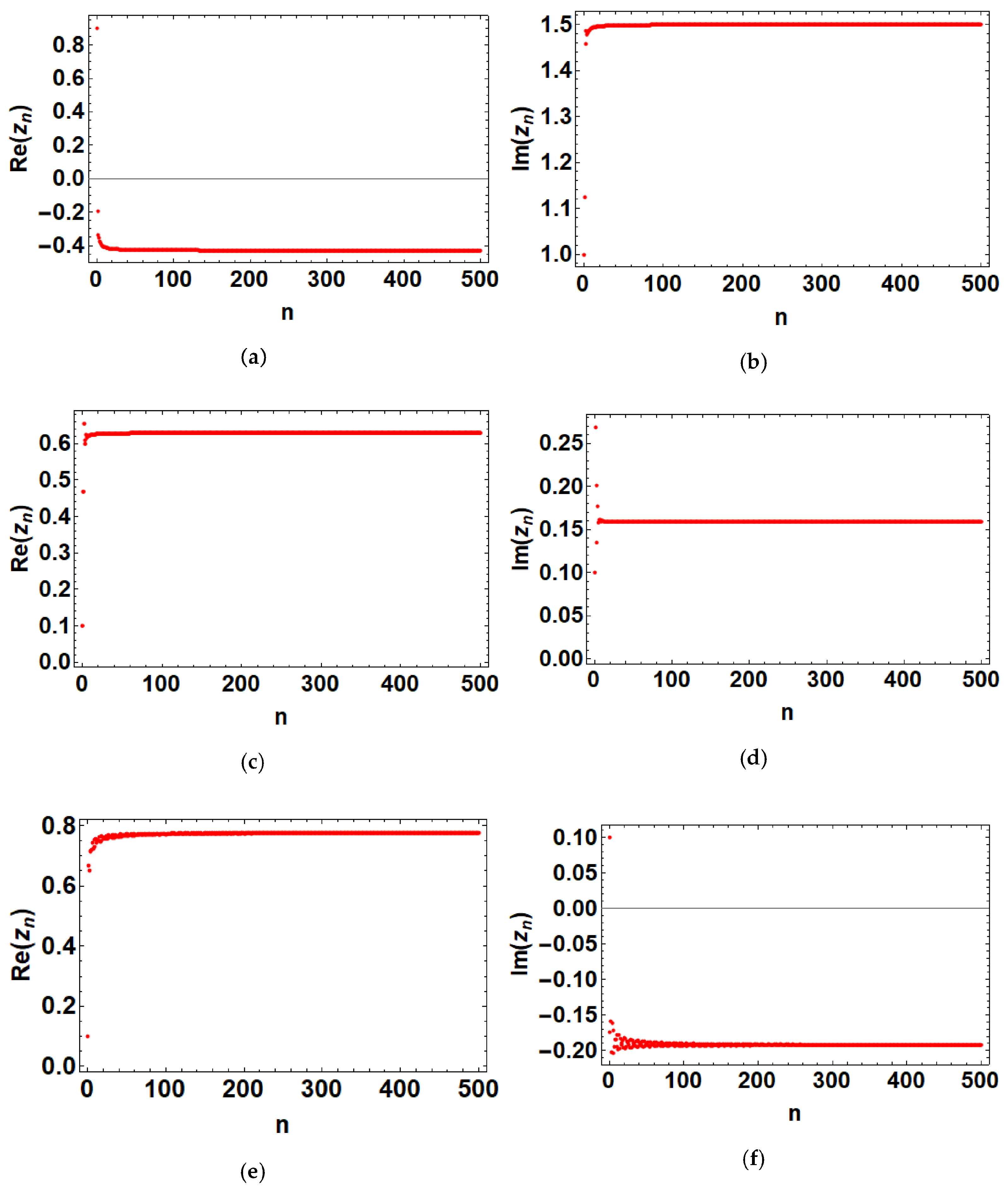
3.1. Stability Analysis of Fixed Points

Theorem 4.

The fractional complex cosine map (6) has a locally asymptotically stable fixed point $z^{*}$ if and only if:

$$\left|{(-1)}^{m+1}p{z}^{{*}^{p-1}}\right|<{(2cos\frac{Arg\left({(-1)}^{m+1}p{z}^{{*}^{p-1}}\right)-\pi }{2-\alpha })}^{\alpha },\left|Arg\left({(-1)}^{m+1}p{z}^{{*}^{p-1}}\right)\right|>\frac{\alpha \pi }{2}.$$

(7)

Proof. 

Let $\delta \left(t\right)=z\left(t\right)-z^{*}$ and consider the following linearized map derived from Equation (6):

$$\begin{array}{cc}\hfill {}^C{\Delta }_a^{\alpha }\delta \left(t\right)& =-p{z}^{{*}^{p-1}}sin[z^{{*}^p}+q]\delta (t+\alpha -1),\hfill \\ \hfill & ={(-1)}^{m+1}p{z}^{{*}^{p-1}}\delta (t+\alpha -1),\hfill \\ \hfill & =\lambda \delta (t+\alpha -1).\hfill \end{array}$$

(8)

The real and imaginary parts of (8) are separated as follows

$${}^C{\Delta }_a^{\alpha }{\delta }_r\left(t\right)+i^C{\Delta }_a^{\alpha }{\delta }_i\left(t\right)=({\lambda }_r+i{\lambda }_i)({\delta }_r(t+\alpha -1)+i{\delta }_i(t+\alpha -1)),$$

and hence the following two dimensional discrete fractional system is obtained

$$\begin{array}{cc}\hfill {}^C{\Delta }_a^{\alpha }{\delta }_r\left(t\right)& ={\lambda }_r{\delta }_r(t+\alpha -1)-{\lambda }_i{\delta }_i(t+\alpha -1),\hfill \\ \hfill {}^C{\Delta }_a^{\alpha }{\delta }_i\left(t\right)& ={\lambda }_i{\delta }_r(t+\alpha -1)+{\lambda }_r{\delta }_i(t+\alpha -1).\hfill \end{array}$$

The above system can be expressed in the form

$$\left(\begin{array}{c}{}^C{\Delta }_a^{\alpha }{\delta }_r\left(t\right)\\ {}^C{\Delta }_a^{\alpha }{\delta }_i\left(t\right)\end{array}\right)=\left(\begin{array}{cc}{\lambda }_r& -{\lambda }_i\\ {\lambda }_i& {\lambda }_r\end{array}\right)\left(\begin{array}{c}{\delta }_r(t+\alpha -1)\\ {\delta }_i(t+\alpha -1)\end{array}\right),$$

(9)

where the eigenvalues of the $2\times 2$ coefficients matrix is found to be $\mathsf{\Lambda }={\lambda }_r\pm \mathtt{i}{\lambda }_i=\lambda ,$$\overline{\lambda }.$

Let

$$B=\left(\begin{array}{cc}{\lambda }_r& -{\lambda }_i\\ {\lambda }_i& {\lambda }_r\end{array}\right),$$

with $tr\left(B\right)=2{\lambda }_r$ and $det\left(B\right)={\lambda }_r^2+{\lambda }_i^2>0,$ then the origin of (9) satisfies the following conditions for asymptotic stability:

$$\sqrt{{\lambda }_r^2+{\lambda }_i^2}<{(2cos\frac{\left|{cot}^{-1}\left(\frac{{\lambda }_r}{{\lambda }_i}\right)\right|-\pi }{2-\alpha })}^{\alpha },\left|{cot}^{-1}(\frac{{\lambda }_r}{{\lambda }_i})\right|>\frac{\alpha \pi }{2}.$$

Equivalently,

$$\left|{(-1)}^{m+1}p{z}^{{*}^{p-1}}\right|<{(2cos\frac{\left|Arg\left({(-1)}^{m+1}p{z}^{{*}^{p-1}}\right)\right|-\pi }{2-\alpha })}^{\alpha },\left|Arg\left({(-1)}^{m+1}p{z}^{{*}^{p-1}}\right)\right|>\frac{\alpha \pi }{2}.$$

In particular, satisfying the above conditions implies that $∥\delta \left(t\right)∥=O\left(t^{-\alpha }\right)$ as $t\to \infty$, i.e., the solutions ${\delta }_r$ and ${\delta }_i$ algebraically decay to zero in the way that $z^{*}$ is locally asymptotically stable for the fractional complex map (6). □

Corollary 1.

For $p=1$ and $m=0,$ the fixed point $z^{*}=\frac{\pi }{2}-q$ is locally asymptotically stable when $0<\alpha \le 1$.

Proof. 

For $p=1$ and $m=0,$ we obtain ${(-1)}^{m+1}p{z}^{{*}^{p-1}}=-1$, and so $\left|Arg\left({(-1)}^{m+1}p{z}^{{*}^{p-1}}\right)\right|=\pi .$ Thus the conditions (7) reduce to

$$1<2^{\alpha },\pi >\frac{\alpha \pi }{2},$$

which are satisfied at $0<\alpha \le 1.$ □

Corollary 2.

For $p=2$ and $m=0,$ the fixed points $z^{*}={\left|\frac{\pi }{2}-q\right|}^{\frac{1}{2}}{e}^{i\frac{{\theta }^{*}}{2}}$ and ${\left|\frac{\pi }{2}-q\right|}^{\frac{1}{2}}{e}^{i\frac{{\theta }^{*}+2\pi }{2}}$ are locally asymptotically stable when

$${\left|\frac{\pi }{2}-q\right|}^{\frac{1}{2}}<2^{\alpha -1}{(cos\frac{\left|{\displaystyle \frac{{\theta }^{*}}{2}}+\pi \right|-\pi }{2-\alpha })}^{\alpha },\left|{\displaystyle \frac{{\theta }^{*}}{2}}+\pi \right|>\frac{\alpha \pi }{2},$$

and

$${\left|\frac{\pi }{2}-q\right|}^{\frac{1}{2}}<2^{\alpha -1}{(cos\frac{\left|{\displaystyle \frac{{\theta }^{*}}{2}}+2\pi \right|-\pi }{2-\alpha })}^{\alpha },\left|{\displaystyle \frac{{\theta }^{*}}{2}}+2\pi \right|>\frac{\alpha \pi }{2}.$$

Proof. 

For $p=2$ and $m=0,$ we obtain ${(-1)}^{m+1}p{z}^{{*}^{p-1}}=2{\left|\frac{\pi }{2}-q\right|}^{\frac{1}{2}}{e}^{i(\frac{{\theta }^{*}}{2}+\pi )},$ $2{\left|\frac{\pi }{2}-q\right|}^{\frac{1}{2}}{e}^{i(\frac{{\theta }^{*}}{2}+2\pi )}$ and hence $\left|Arg\left({(-1)}^{m+1}p{z}^{{*}^{p-1}}\right)\right|=\left|{\displaystyle \frac{{\theta }^{*}}{2}}+\pi \right|,$ $\left|{\displaystyle \frac{{\theta }^{*}}{2}}+2\pi \right|,$ for the two fixed points, respectively. Thus the conditions (7) reduce to

$$2{\left|\frac{\pi }{2}-q\right|}^{\frac{1}{2}}<{(2cos\frac{\left|{\displaystyle \frac{{\theta }^{*}}{2}}+\pi \right|-\pi }{2-\alpha })}^{\alpha },\left|{\displaystyle \frac{{\theta }^{*}}{2}}+\pi \right|>\frac{\alpha \pi }{2},$$

for the first fixed point and for the second fixed point it follows that

$$2{\left|\frac{\pi }{2}-q\right|}^{\frac{1}{2}}<{(2cos\frac{\left|{\displaystyle \frac{{\theta }^{*}}{2}}+2\pi \right|-\pi }{2-\alpha })}^{\alpha },\left|{\displaystyle \frac{{\theta }^{*}}{2}}+2\pi \right|>\frac{\alpha \pi }{2}.$$

□

The previous theoretical results are validated using numerical simulations. In the first case, let $p=1,\alpha =0.95,$ $q=2-1.5i$ and $m=0.$ Then the fixed point $z^{*}=-0.429204+1.5i$ is locally asymptotically stable according to Corollary 2, see Figure 1a,b. Now, consider the second case where $p=2,\alpha =0.85,$ $q=1.2-0.2i$ and $m=0,$ and the fixed points are $0.629322+0.158901i$ and $-0.629322-0.158901i.$ The conditions for asymptotic stability indicate that the first fixed point $0.629322+0.158901i$ is asymptotically stable whereas the second one is unstable, as shown in Figure 1c,d. In the third case, taking $p=2,\alpha =0.7,$ $q=1+0.3i$ and $m=0,$ the fixed points are found to be $0.7796-0.1924i$ and $-0.779624+0.1924i.$ Stability conditions reveal that the first fixed point is asymptotically stable while the second one is unstable. Numerical simulations in Figure 1e,f verify these predictions.

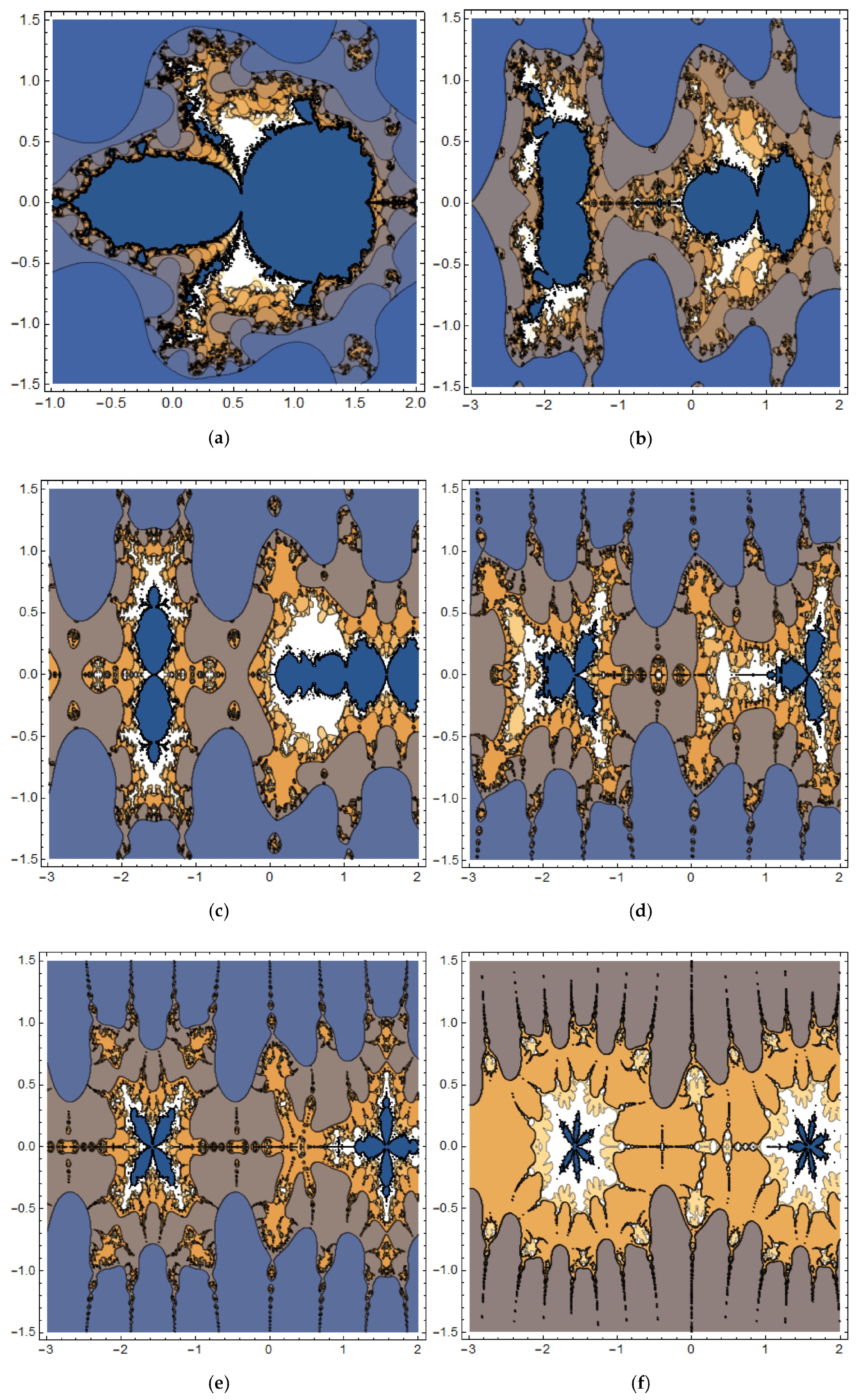
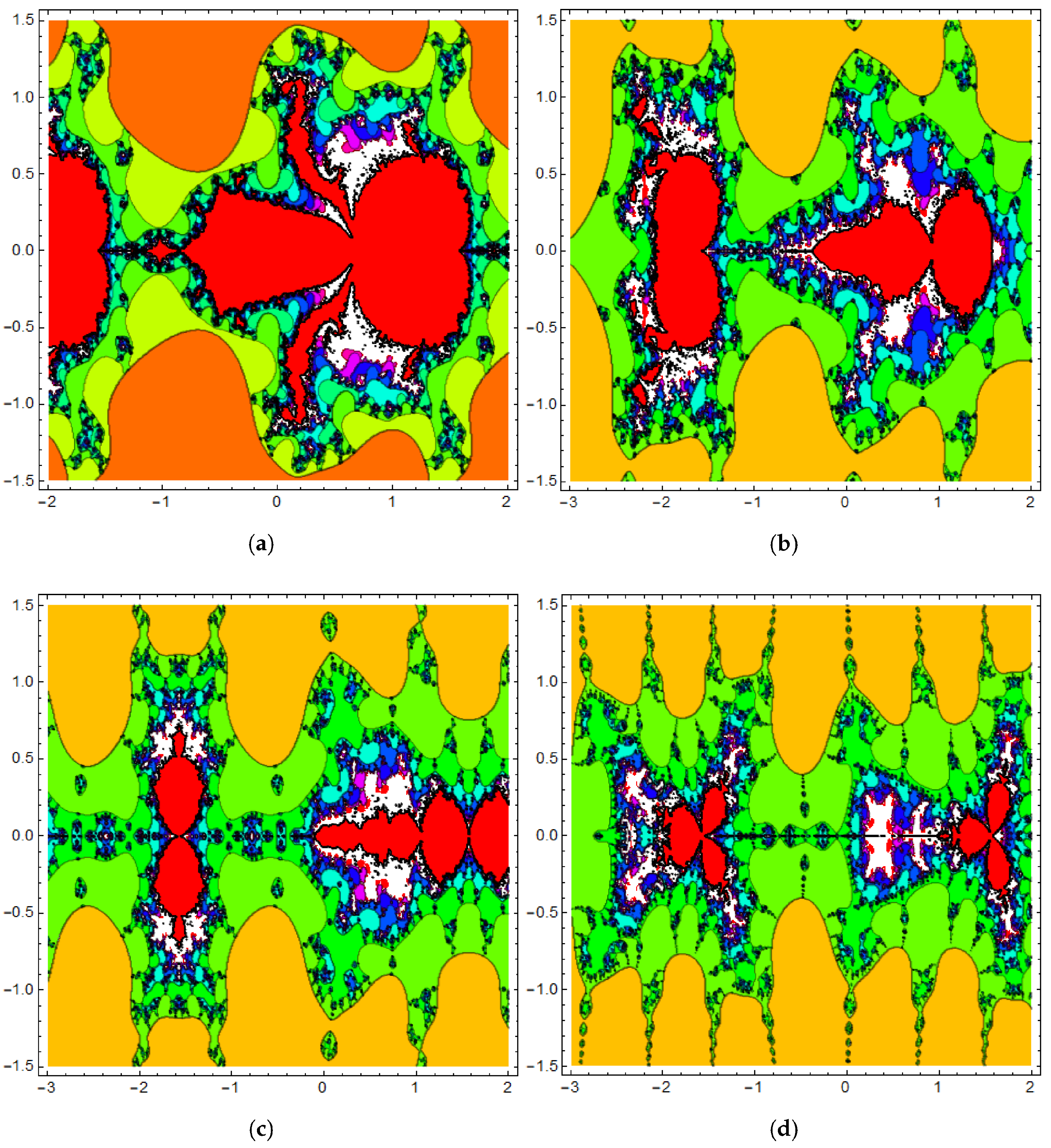
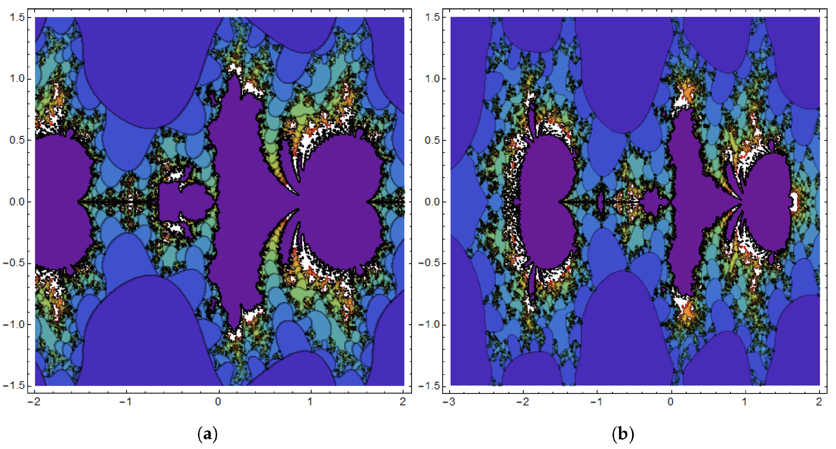
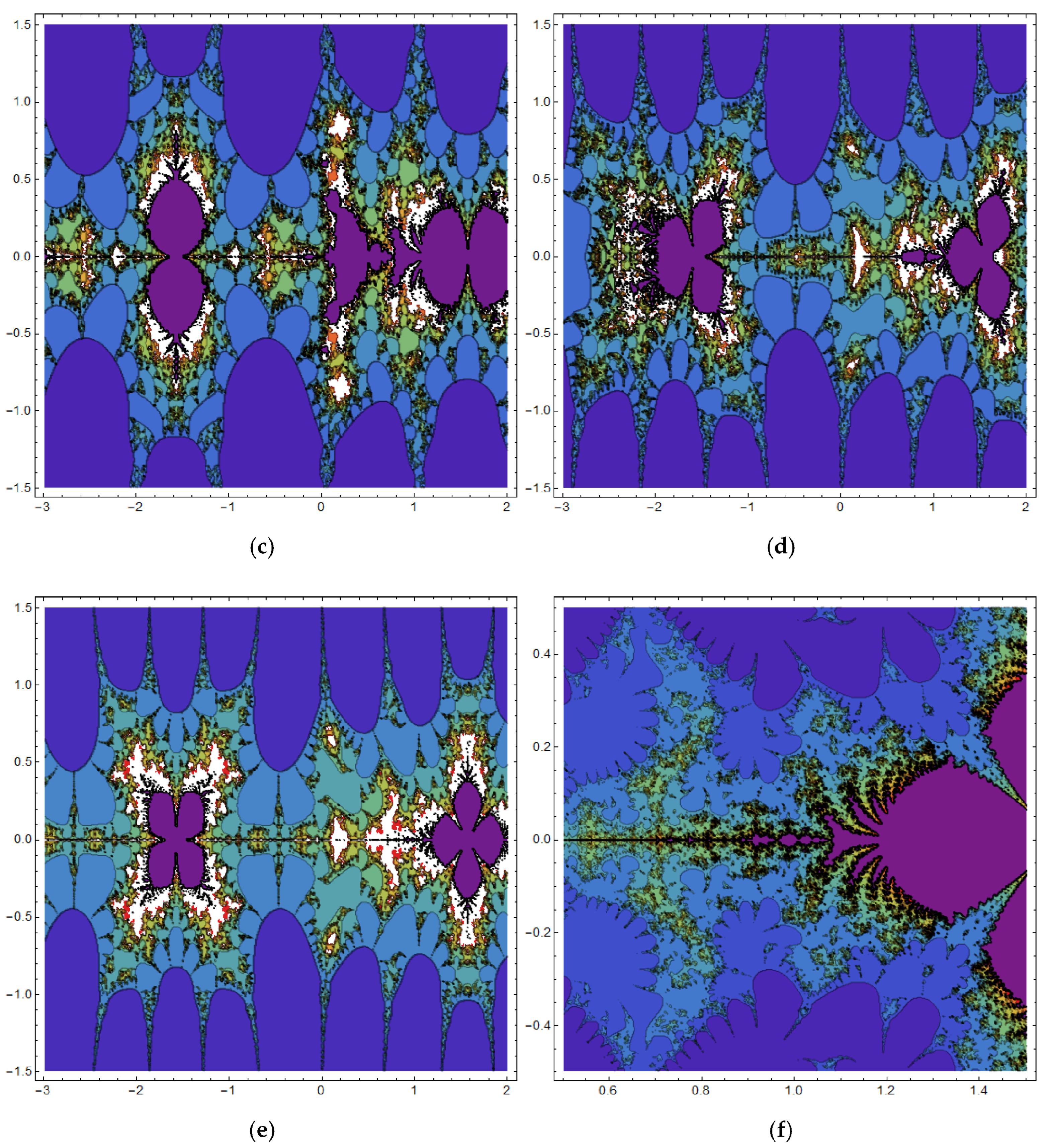
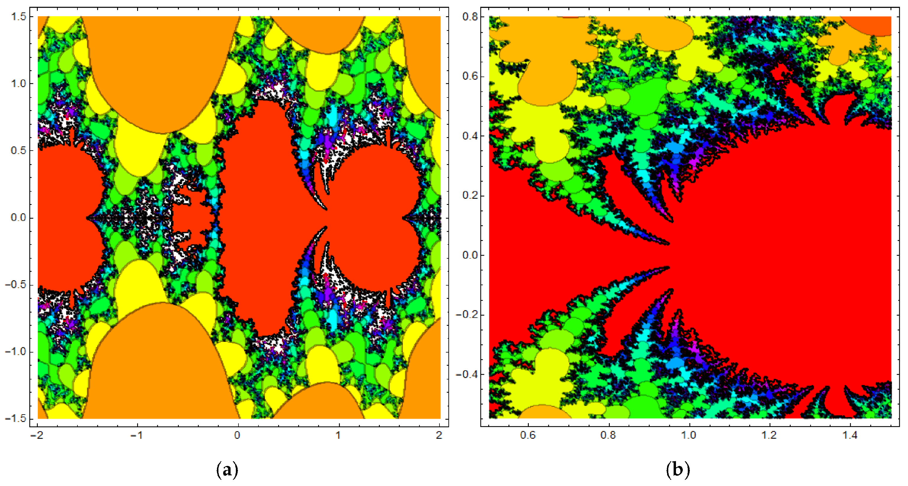
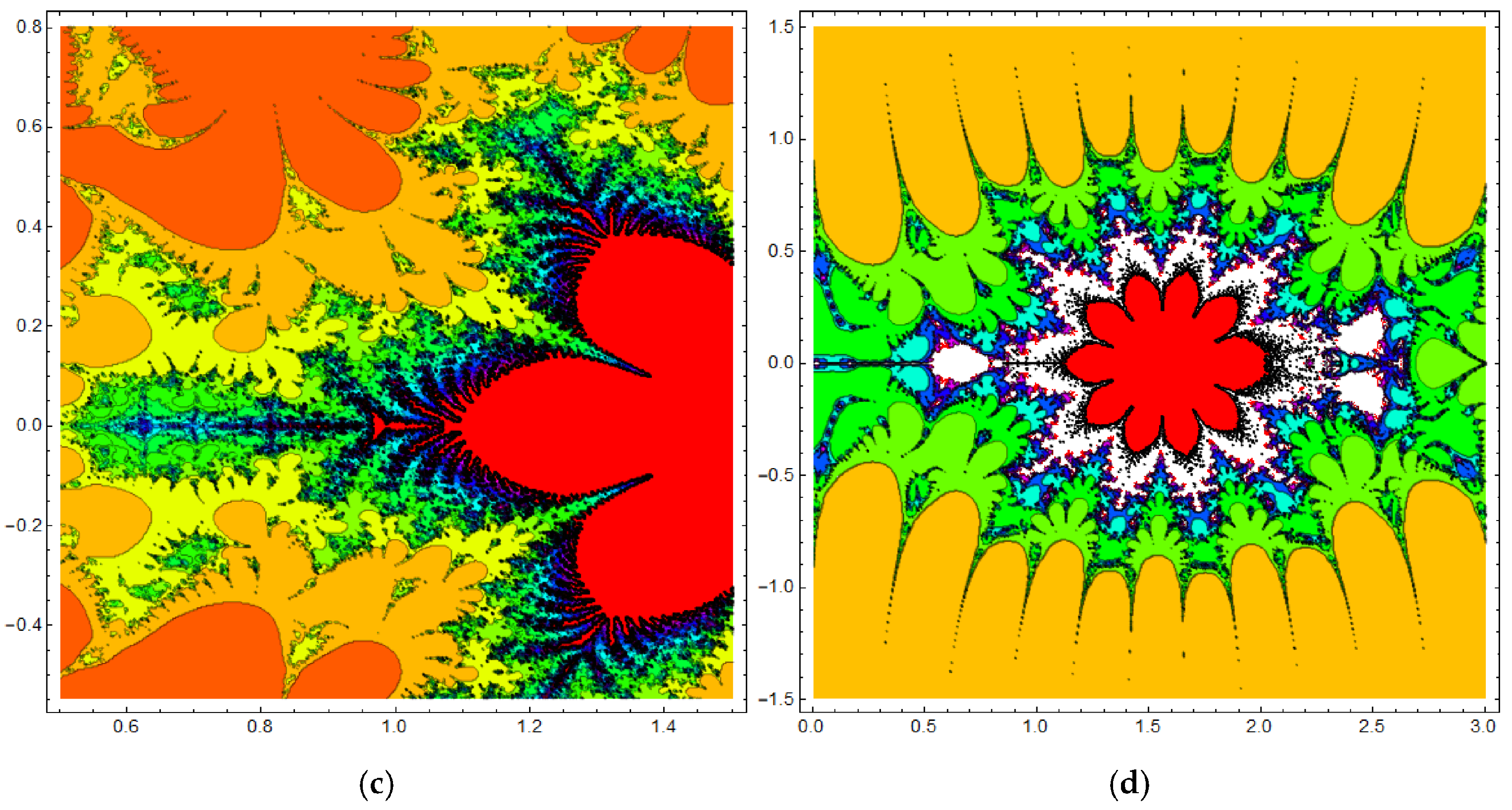
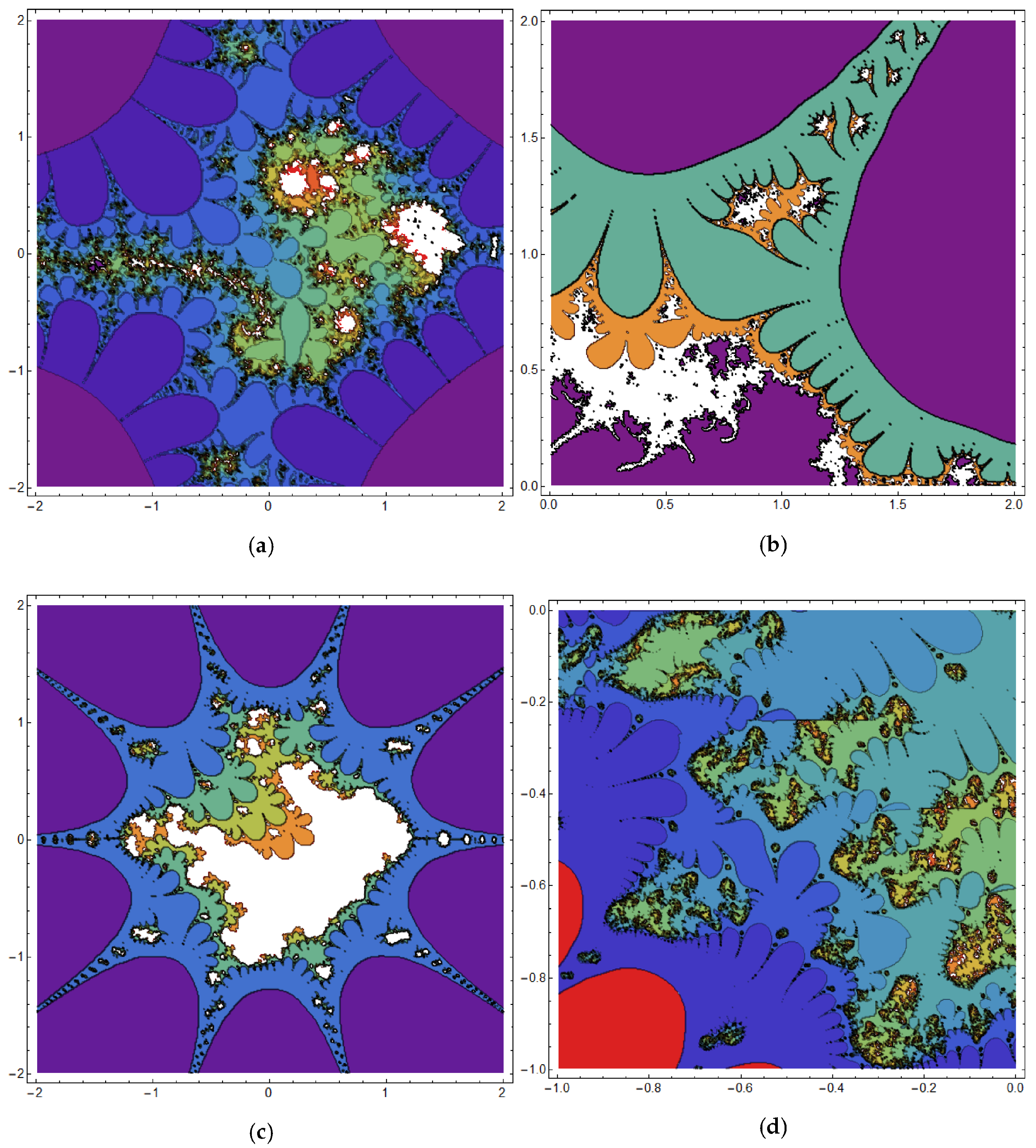
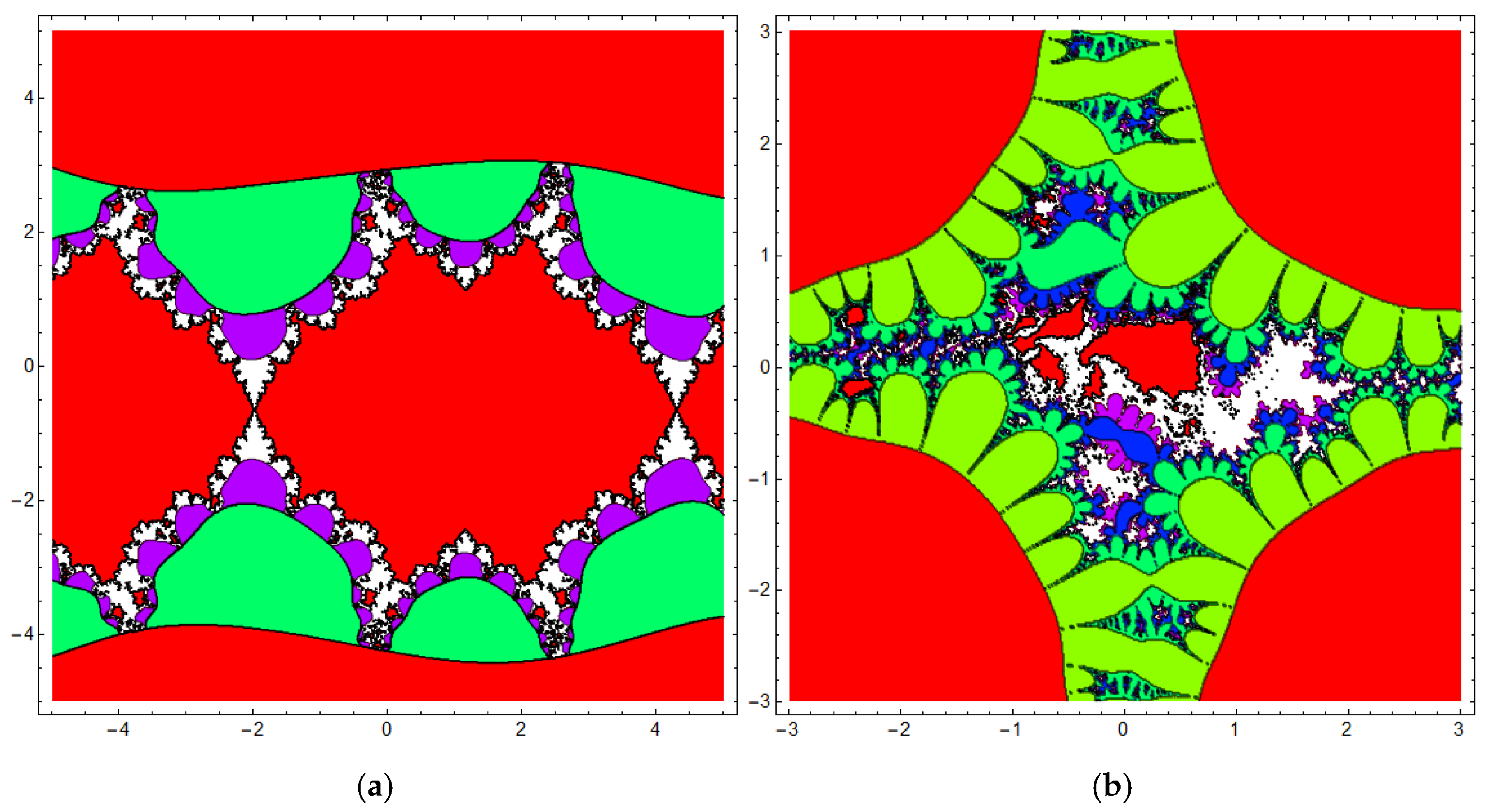
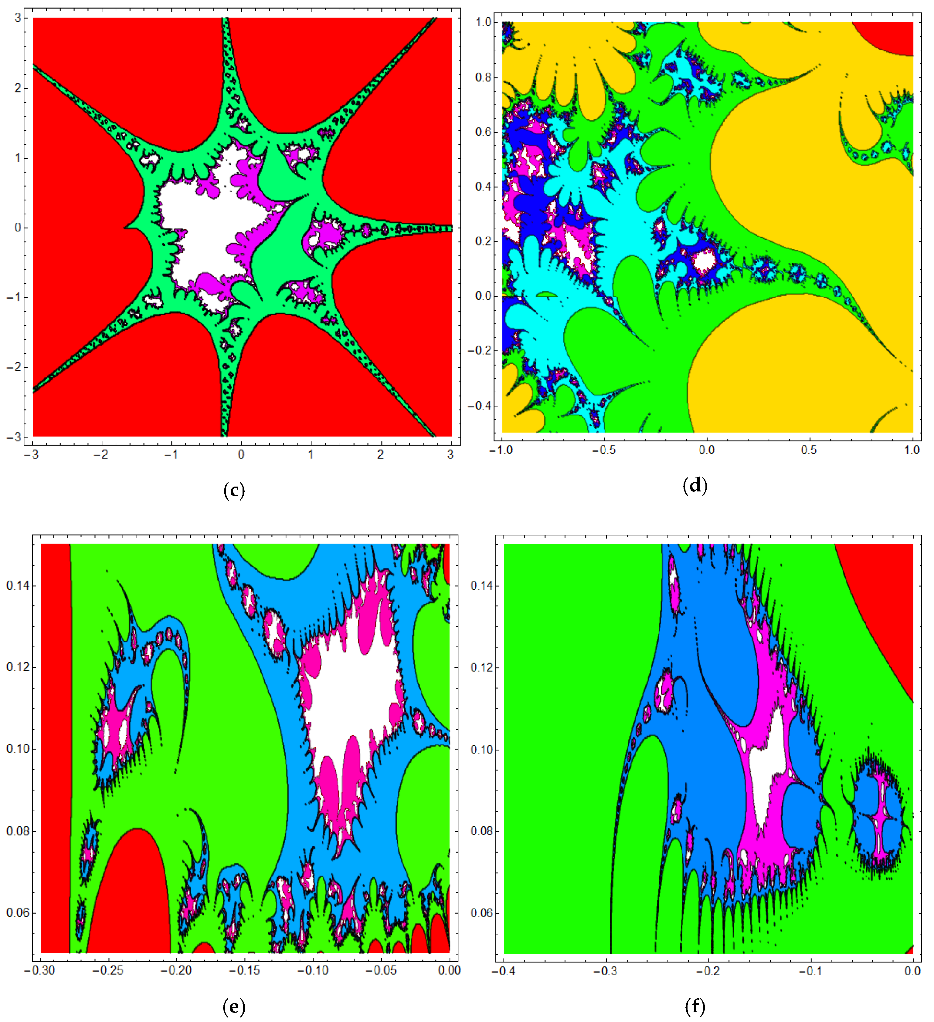
3.2. The Fractional Cosine Map Generates Fractal Sets

We extend the ideas of Julia and Mandelbrot fractal sets to the more general case of discrete fractional-order complex-valued maps. Consider the following fractional-order map

$${}^C{\Delta }_a^{\alpha }z\left(t\right)=f(z(t+\alpha -1),q),$$

(10)

where $f:\mathbb{C}\to \mathbb{C}$ and $q\in \mathbb{C},$ then the Julia set induced by (10) is defined as follows [9,10,11]:

Definition 2.

The filled-in Julia set of discrete fractional map (10) is the set Ψ of initial points $z\in \mathbb{C}$ whose evolutions under (10) are limited. The boundary of Ψ, i.e., $\partial \mathsf{\Psi }$, is referred to as the Julia set of discrete fractional map (10) and it is denoted by $J_f^{\alpha }.$

The key properties of Julia set $J_f^{\alpha }$ are listed below [9,10,11]:

(1) $J_f^{\alpha }\ne ⌀$, i.e., it is a non-empty set.

(2) $J_f^{\alpha }$ is fully invariant with respect to (10) in both forward and backward directions of iterations.

(3) Assume that the fractional map (10) has an attractive fixed point of period p at some specific values of $\alpha ,$ then $J_f^{\alpha }$ contains the basin of attraction for this fixed point, namely, $\partial {\beta }_p^{\alpha }.$ The same is true for infinity fixed point.

The Mandelbrot set, introduced by Benoit Mandelbrot in 1979 [9,10], is generalized to our fractional case in the way that the Mandelbrot set ${\mathsf{\Phi }}_f^{\alpha }$ is composed of the set of points in the plane of complex-valued parameter q at which the evolution from initial point $z\left(0\right)=0$ is bounded at the specified fixed value of $\alpha .$

The quantification of fractal properties of Julia and Mandelbrot sets can be carried out by calculating the associated space filling capacity or dimension. The well-known box-counting dimension is the most accessible among scientists and it can be defined as follows:

Definition 3.

For non-empty bounded subset Ω of ${\mathbb{R}}^n,$ consider the collections of boxes with side lengths ϵ required to cover Ω. The Minkowski–Bouligand dimension or the box-counting dimension is defined as

$${dim}_{\mathsf{\Omega }}=\underset{ϵ\to 0}{lim}\frac{log\left(N_{ϵ}\right)}{log(1/ϵ)},$$

where $N_{ϵ}$ is the number of boxes to cover $\mathsf{\Omega }.$ In addition, the lower box dimension (lower Minkowski dimension) and the upper box dimension (Kolmogorov dimension) of Ω are also defined by

$${\underline{dim}}_{\mathsf{\Omega }}=\underset{ϵ\to 0}{\underline{lim}}\frac{log\left(N_{ϵ}\right)}{log(1/ϵ)},{\overline{dim}}_{\mathsf{\Omega }}=\overline{{lim}_{ϵ\to 0}}\frac{log\left(N_{ϵ}\right)}{log(1/ϵ)},$$

respectively.

Numerical simulations are carried out to explore the generation of Mandelbrot and Julia sets from the dynamics of the proposed generalized fractional cosine map. The results for different values of the fractional order $\alpha$, the constant q, and the exponent p are shown in the next table. In addition, Table 1 provides the box-counting dimensions for the various simulation scenarios investigated.

Table 1. Summary of cases considered in numerical simulations and the associated fractal dimensions.

Figure	Fractal Set	Parameters	Fractal Dimension
Figure 2	Mandelbrot sets	$\alpha =1,$ different values of $p.$	$1.5244,1.582,1.6148,1.6594,1.5615,1.5442$
Figure 3	Mandelbrot sets	$\alpha =0.9,$ different values of $p.$	$1.8838,1.8836,1.8994,1.8893$
Figure 4	Mandelbrot sets	$\alpha =0.75,$ different values of $p.$	$1.8643,1.8828,1.8748,1.909,1.8762,1.8967$
Figure 5	Mandelbrot sets	$\alpha =0.5,$ different values of $p.$	$1.633,1.6722,1.6782,1.6838,1.6857,1.6337,1.5536$
Figure 6	Mandelbrot sets	$\alpha =0.3,$ different values of $p.$	$1.8572,1.8908,1.8904,1.5768$
Figure 7	Julia sets	$\alpha =1,$ different values of p and $q.$	$1.8426,1.8665,1.4931,1.5469$
Figure 8	Julia sets	$\alpha =0.8,$ different values of p and $q.$	$1.8765,1.489,1.8525,1.8503$
Figure 9	Julia sets	$\alpha =0.5,$ different values of p and $q.$	$1.5016,1.8864,1.5078,1.4836,1.8021,1.8034$

Table 1. Summary of cases considered in numerical simulations and the associated fractal dimensions.

Figure	Fractal Set	Parameters	Fractal Dimension
Figure 2	Mandelbrot sets	$\alpha =1,$ different values of $p.$	$1.5244,1.582,1.6148,1.6594,1.5615,1.5442$
Figure 3	Mandelbrot sets	$\alpha =0.9,$ different values of $p.$	$1.8838,1.8836,1.8994,1.8893$
Figure 4	Mandelbrot sets	$\alpha =0.75,$ different values of $p.$	$1.8643,1.8828,1.8748,1.909,1.8762,1.8967$
Figure 5	Mandelbrot sets	$\alpha =0.5,$ different values of $p.$	$1.633,1.6722,1.6782,1.6838,1.6857,1.6337,1.5536$
Figure 6	Mandelbrot sets	$\alpha =0.3,$ different values of $p.$	$1.8572,1.8908,1.8904,1.5768$
Figure 7	Julia sets	$\alpha =1,$ different values of p and $q.$	$1.8426,1.8665,1.4931,1.5469$
Figure 8	Julia sets	$\alpha =0.8,$ different values of p and $q.$	$1.8765,1.489,1.8525,1.8503$
Figure 9	Julia sets	$\alpha =0.5,$ different values of p and $q.$	$1.5016,1.8864,1.5078,1.4836,1.8021,1.8034$

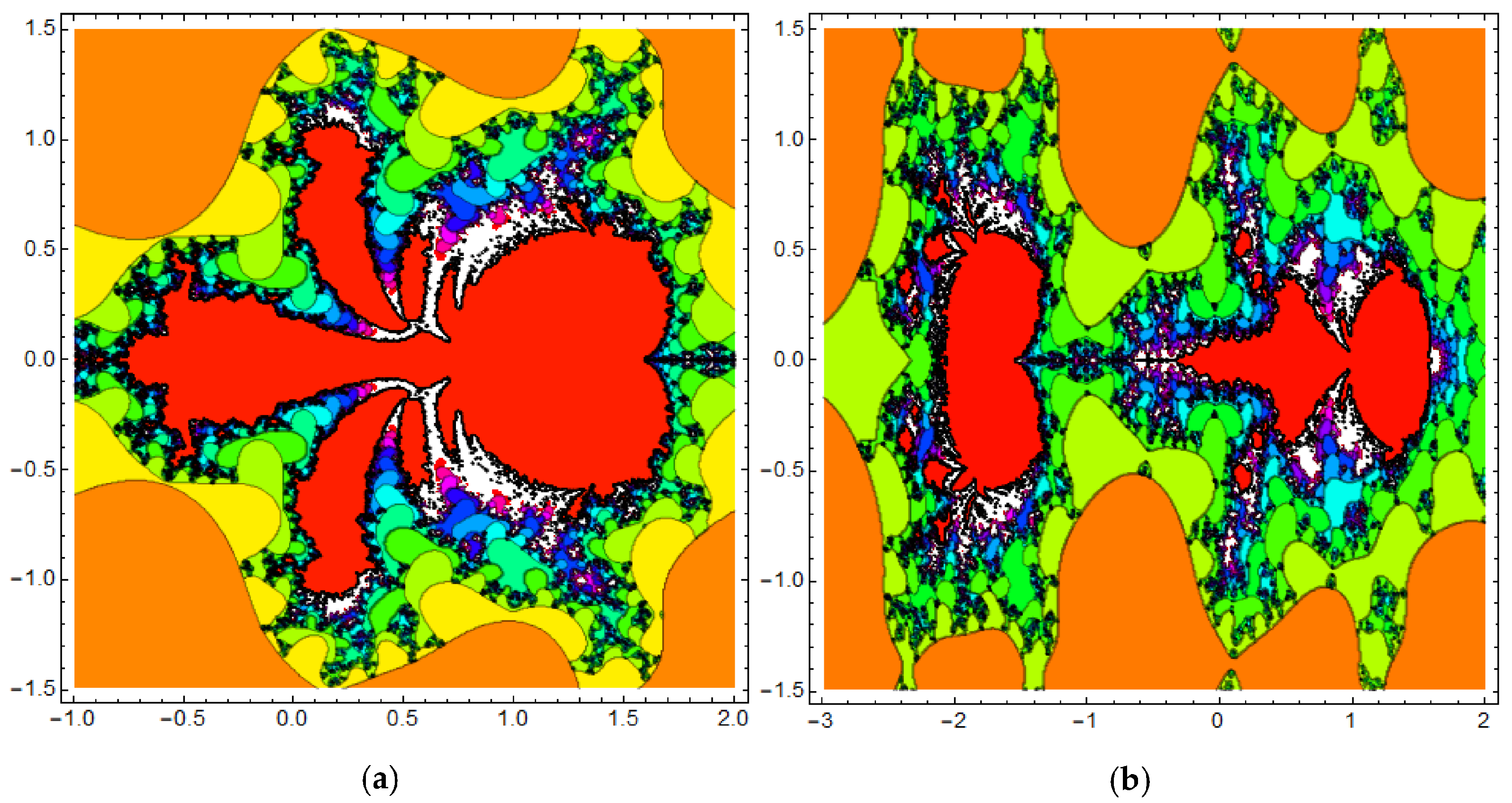
4. The Control and Synchronization of Julia Sets

This section examines the regulation and synchronization of Julia sets generated by the fractional-order cosine map. This section begins with a brief mathematical overall view.

Consider two different fractional-order cosine maps The first is called the master (driving) map and has the output $z_1\left(t\right)$ whereas the second map is referred to as the slave (response) map and it gives the output $z_2\left(t\right)$.

Definition 4.

The synchronization is said to be achieved between $z_1\left(t\right)$ and $z_2\left(t\right)$ if $z_2\to z_1$ as $t\to \infty$. Equivalently, it can be written as [11,12,13]

$$\underset{t\to \infty }{lim}\left|z_2\left(t\right)-z_1\left(t\right)\right|=0.$$

The synchronization of two solution trajectories indicates that their convergence and divergence characteristics are identical. Let $J_{f_1}^{\alpha }$ and $J_{f_2}^{\alpha }$ denote the Julia sets of fractional master and fractional slave maps, respectively, where they have fractional order $\alpha$. The definition of synchronization between two Julia sets is as follows [11,12,13,14].

Definition 5.

The asymptotic synchronization of two Julia sets $J_{f_1}^{\alpha }$ and $J_{f_2}^{\alpha }$ is achieved if

$$\underset{t\to \infty }{lim}(J_{f_1}^{\alpha }\cup J_{f_2}^{\alpha }-J_{f_1}^{\alpha }\cap J_{f_2}^{\alpha })=⌀.$$

4.1. Control of Julia Sets Generated by the Fractional Cosine Map

The Julia sets created by the fractional cosine map are controlled by varying the type of stability of a particular fixed point on the map. The proposed form of the feedback controller is

$$\upsilon \left(t\right)=-\kappa (z\left(t\right)-\overline{z})-cos[z{(t+\alpha -1)}^p+q],$$

(11)

where $\overline{z}$ is the target fixed point and the complex-valued controller gain $\kappa ={\kappa }_r+i{\kappa }_i$ is calculated as follows:

Theorem 5.

Suppose that the feedback controller (11) satisfies the following conditions

$${\kappa }_r>0,\sqrt{{\kappa }_r^2+{\kappa }_i^2}<2^{\alpha },$$

subsequently, the unstable fixed point $\overline{z}$ of controlled fractional-order cosine map

$${}^C{\Delta }_a^{\alpha }z\left(t\right)=cos[z{(t+\alpha -1)}^p+q]+\upsilon (t+\alpha -1),$$

is stabilized by changing the Julia set in its neighborhood.

Proof. 

Using control signal (11), the controlled fractional cosine map can be written as:

$${}^C{\Delta }_a^{\alpha }z\left(t\right)=-\kappa (z(t+\alpha -1)-\overline{z}).$$

(12)

Let $u\left(t\right)=z\left(t\right)-\overline{z},$ then (12) represents a structure

$${}^C{\Delta }_a^{\alpha }u\left(t\right)=-\kappa u(t+\alpha -1),$$

and the associated real-valued two dimensional fractional map is obtained as

$$\begin{array}{cc}\hfill {}^C{\Delta }_a^{\alpha }{u}_r\left(t\right)& =-{\kappa }_r{u}_r(t+\alpha -1)+{\kappa }_i{u}_i(t+\alpha -1),\hfill \\ \hfill {}^C{\Delta }_a^{\alpha }{u}_i\left(t\right)& =-{\kappa }_i{u}_r(t+\alpha -1)-{\kappa }_r{u}_i(t+\alpha -1).\hfill \end{array}$$

Define matrix J by

$$J=\left(\begin{array}{cc}-{\kappa }_r& {\kappa }_i\\ -{\kappa }_i& -{\kappa }_r\end{array}\right),$$

and hence the eigenvalues of J are given by $-{\kappa }_r\pm i{\kappa }_i.$ The sufficient conditions for local asymptotic stability of ${\kappa }_r>0$ and $\sqrt{{\kappa }_r^2+{\kappa }_i^2}<2^{\alpha }.$ □

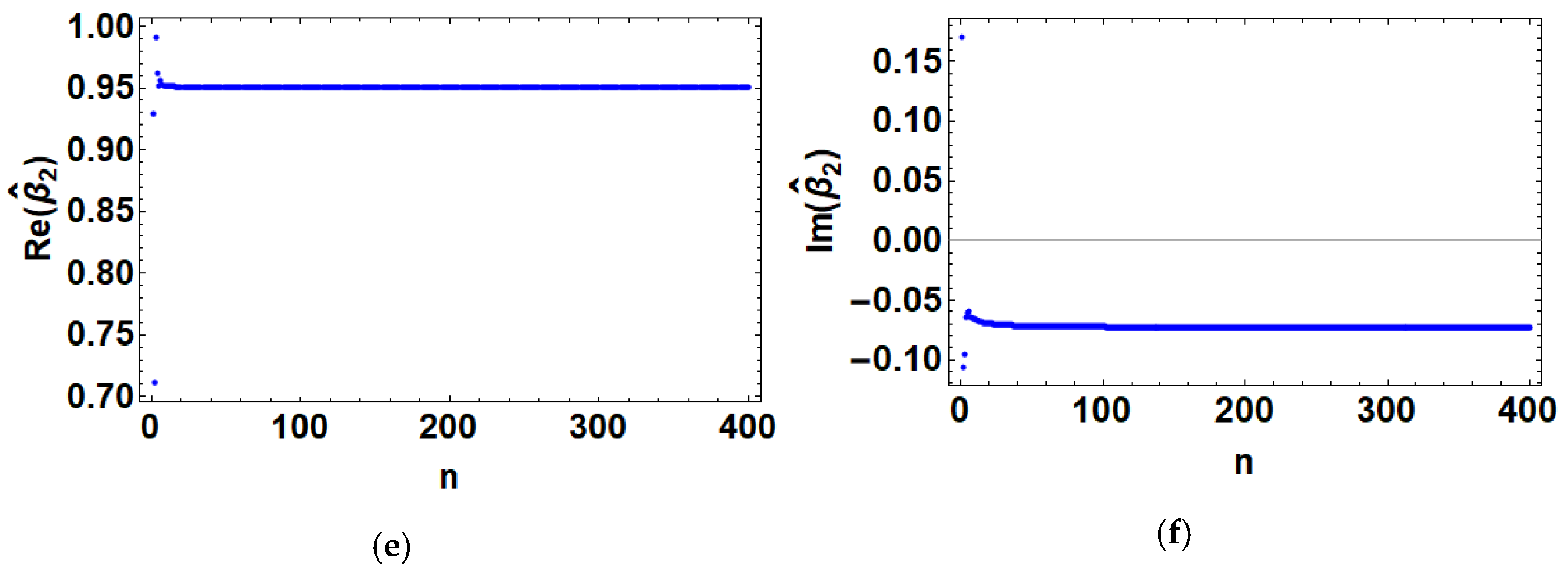
4.2. Synchronization of Julia Sets

Assume the driving system has the following configuration:

$${}^C{\Delta }_a^{\alpha }{z}_1\left(t\right)=cos[z_1{(t+\alpha -1)}^p+q_1],$$

(13)

and take into account the following response system

$${}^C{\Delta }_a^{\alpha }{z}_2\left(t\right)=cos[z_2{(t+\alpha -1)}^p+q_2]+\rho (z_1,z_2,t+\alpha -1),$$

(14)

where $\rho (z_1,z_2,t+\alpha -1)$ is an appropriate controller to be designed.

Now, two different scenarios will be investigated in the following two theorems. The first one involves the case where the values of the constants $q_1$ and $q_2$ are known a priori.

Theorem 6.

Suppose that the values of constants $q_1$ and $q_2$ in the two fractional maps (13) and (14), respectively, are known. Then, the following controller

$$\rho (z_1,z_2,t+\alpha -1)=cos[z_1{(t+\alpha -1)}^p+q_1]-cos[z_2{(t+\alpha -1)}^p+q_2]-\gamma (z_2(t+\alpha -1)-z_1(t+\alpha -1)),$$

(15)

with gain $\gamma ={\gamma }_r+i{\gamma }_i$ satisfying $\left|\gamma \right|<2^{\alpha }$ and ${\gamma }_r>0,$ can realize Julia set synchronization between the driving system (13) and the response system (14) for any initial condition.

Proof. 

One can obtain the fractional error map by subtracting (13) from (14) which can be written as

$$\begin{array}{cc}\hfill {}^C{\Delta }_a^{\alpha }e\left(t\right)& =cos[z_2{(t+\alpha -1)}^p+q_2]-cos[z_1{(t+\alpha -1)}^p+q_1]+\rho (z_1,z_2,t+\alpha -1),\hfill \\ \hfill e\left(t\right)& =z_2\left(t\right)-z_1\left(t\right).\hfill \end{array}$$

By substituting from (15) into the above error map, we get

$${}^C{\Delta }_a^{\alpha }e\left(t\right)=-\gamma e(t+\alpha -1),$$

or

$${}^C{\Delta }_a^{\alpha }(e_r\left(t\right)+e_i\left(t\right))=(-{\gamma }_r-i{\gamma }_i)(e_r(t+\alpha -1)+i{e}_i(t+\alpha -1)),$$

which can be changed into the 2D system

$$\begin{array}{cc}\hfill {}^C{\Delta }_a^{\alpha }{e}_r\left(t\right)& =-{\gamma }_r{e}_r(t+\alpha -1)+{\gamma }_i{e}_i(t+\alpha -1),\hfill \\ \hfill {}^C{\Delta }_a^{\alpha }{e}_i\left(t\right)& =-{\gamma }_i{e}_r(t+\alpha -1)-{\gamma }_r{e}_i(t+\alpha -1).\hfill \end{array}$$

The eigenvalues of the above system are found as $-{\gamma }_r\pm i{\gamma }_i$ which imply that the asymptotic stability conditions are achieved if $\left|\gamma \right|<2^{\alpha }$ and ${\gamma }_r>0.$ □

The second scenario involves the case where the value of constant $q_1$ is unknown and, therefore, an adaptive controller is to be designed along with complex-valued update laws to realize the synchronization.

Theorem 7.

Suppose that the value of constants $q_1$ in the fractional map (13) is unknown. Then, the following controller

$$\begin{array}{cc}\hfill \rho (z_1,z_2,t+\alpha -1)& ={\widehat{\beta }}_1(t+\alpha -1)cos\left(z_1{(t+\alpha -1)}^p\right)+{\widehat{\beta }}_2(t+\alpha -1)sin\left(z_1{(t+\alpha -1)}^p\right)\hfill \\ \hfill & -cos[z_2{(t+\alpha -1)}^p+q_2]-\gamma e(t+\alpha -1),\hfill \end{array}$$

(16)

along with the following update laws

$$\begin{array}{cc}\hfill \Delta {\widehat{\beta }}_1\left(n\right)& =-\frac{{\eta }_1(e(n+1)cos\left(z_1{\left(n\right)}^p\right)-e\left(n\right)cos\left(z_1{(n+1)}^p\right))}{cos\left(z_1{(n+1)}^p\right)cos\left(z_1{\left(n\right)}^p\right)},\hfill \end{array}$$

(17)

$$\begin{array}{cc}\hfill \Delta {\widehat{\beta }}_2\left(n\right)& =-\frac{{\eta }_2(e(n+1)sin\left(z_1{\left(n\right)}^p\right)-e\left(n\right)sin\left(z_1{(n+1)}^p\right))}{sin\left(z_1{(n+1)}^p\right)sin\left(z_1{\left(n\right)}^p\right)}\hfill \end{array}$$

(18)

where ${\widehat{\beta }}_1,$${\widehat{\beta }}_2$ are the estimates of $cos\left(q_1\right)$ and $-sin\left(q_1\right),$ respectively, and the complex-valued gains $\gamma ,{\eta }_1$ and ${\eta }_2$ satisfying $\left|\gamma +{\eta }_1+{\eta }_2\right|<2^{\alpha }$ and ${\gamma }_r+{\eta }_{1r}+{\eta }_{2r}>0$ can achieve Julia set synchronization between the driving system (13) and the response system (14) for any initial condition.

Proof. 

The proof is arranged in the following steps. First, the drive map is simplified to the following form:

$$\begin{array}{cc}\hfill {}^C{\Delta }_a^{\alpha }{z}_1\left(t\right)& =cos\left(q_1\right)cos\left(z_1{(t+\alpha -1)}^p\right)-sin\left(q_1\right)sin\left(z_1{(t+\alpha -1)}^p\right)\hfill \\ \hfill & ={\beta }_{1}cos\left(z_1{(t+\alpha -1)}^p\right)+{\beta }_{2}sin\left(z_1{(t+\alpha -1)}^p\right),\hfill \\ \hfill {\beta }_1& =cos\left(q_1\right),{\beta }_2=-sin\left(q_1\right).\hfill \end{array}$$

The fractional error map is then expressed as

$${}^C{\Delta }_a^{\alpha }e\left(t\right)=cos[z_2{(t+\alpha -1)}^p+q_2]-{\beta }_{1}cos\left(z_1{(t+\alpha -1)}^p\right)-{\beta }_{2}sin\left(z_1{(t+\alpha -1)}^p\right)+\rho (z_1,z_2,t+\alpha -1).$$

Second, by substituting (16) into the fractional error map, we obtain

$$\begin{array}{cc}\hfill {}^C{\Delta }_a^{\alpha }e\left(t\right)& =({\widehat{\beta }}_1(t+\alpha -1)-{\beta }_1)cos\left(z_1{(t+\alpha -1)}^p\right)+({\widehat{\beta }}_2(t+\alpha -1)-{\beta }_2)sin\left(z_1{(t+\alpha -1)}^p\right)-\gamma e(t+\alpha -1),\hfill \\ \hfill & ={\tilde{\beta }}_1(t+\alpha -1)cos\left(z_1{(t+\alpha -1)}^p\right)+{\tilde{\beta }}_2(t+\alpha -1)sin\left(z_1{(t+\alpha -1)}^p\right)-\gamma e(t+\alpha -1).\hfill \end{array}$$

In addition, note that

$$\Delta {\widehat{\beta }}_1\left(n\right)=\Delta {\tilde{\beta }}_1\left(n\right),\Delta {\widehat{\beta }}_2\left(n\right)=\Delta {\tilde{\beta }}_2\left(n\right),$$

and hence the update laws (17)–(18) can be solve to give

$${\tilde{\beta }}_1\left(n\right)=-\frac{{\eta }_{1}e\left(n\right)}{cos\left(z_1{\left(n\right)}^p\right)},{\tilde{\beta }}_2\left(n\right)=-\frac{{\eta }_{2}e\left(n\right)}{sin\left(z_1{\left(n\right)}^p\right)}.$$

Third, the error map is, therefore, reduced to

$${}^C{\Delta }_a^{\alpha }e\left(t\right)=-(\gamma +{\eta }_1+{\eta }_2)e(t+\alpha -1),$$

which implies that the corresponding 2D fractional error map in ${\mathbb{R}}^2$ has the eigenvalues $-({\gamma }_r+{\eta }_{1r}+{\eta }_{2r})\pm i({\gamma }_i+{\eta }_{1i}+{\eta }_{2i})$ at the zero fixed point. Therefore, the following conditions are sufficient to confirm the fixed point stability

$$\left|\gamma +{\eta }_1+{\eta }_2\right|<2^{\alpha },{\gamma }_r+{\eta }_{1r}+{\eta }_{2r}>0.$$

□

To validate the theoretical results obtained in this section, numerical simulations are now used. For $p=2,$ $q=1.2-0.2i$ and $\alpha =0.8,$ it can be found that the fixed point $-0.62932-0.1589012i$ is an unstable fixed point for the fractional cosine map (6). Applying the controller (11) with $\overline{z}=-0.62932-0.1589i$ and $\kappa =1,$ the fixed point is stabilized, as shown in Figure 10a,b. In a second example, consider a master system with $p=2,$ $q_1=1.2-0.2i$ and $\alpha =0.9$ while the slave system is supposed to have $p=2,$ $q_2=0.433-0.55i$ and $\alpha =0.9.$ Using the adaptive controller (15) with $\gamma =1+0.3i,$ the synchronization conditions are satisfied and the synchronization between the two systems are achieved. The evolution of the synchronization error with time is illustrated in Figure 10c,d for its real and imaginary parts. The third example involves the more realistic case where the value of $q_1$ is unknown in the master system. The value of $q_2$ in the slave system is set to $0.433-0.55i$ and the other shared values of parameters are $p=2$ and $\alpha =0.85.$ The adaptive controller (16) along with update laws (17)–(18) are employed to achieve the synchronization between the two systems and estimate the unknown values of $cos\left(q_1\right)$ and $-sin\left(q_1\right).$ In the simulations shown in Figure 11, the assigned values to $cos\left(q_1\right)$ and $sin\left(q_1\right)$ are $0.369629+0.18765i$ and $0.950742-0.072956i$, respectively. Figure 11a–f shows the real and imaginary parts of the synchronization error, ${\widehat{\beta }}_1$ and ${\widehat{\beta }}_2.$ The Julia set generated by the controlled map is affected by the stabilization of specific fixed points in the fractional cosine map or the induced synchronization between master/slave systems. For example, Figure 12 depicts the Julia sets generated by the slave fractional cosine map before and after attaining the synchronization state where it is clear that significant changes in its structure are introduced.

5. Conclusions

This research introduces a framework for investigating the fractal and dynamic properties of an extended discrete fractional cosine map with complex values. The Mandelbrot and Julia sets of the proposed map are investigated for a variety of parameters. Julia sets in complex domains: control and synchronization issues discussed. In particular, an efficient adaptive controller is constructed to achieve synchronization when there is an unknown value of the parameter in driving (master system). The proposed map has promising applications in the field of image encryption which can be conducted in future work. Our findings can be used to create a reliable and efficient chaotic color/grayscale image encrypting system. The next step in our future work is to apply the present discrete fractional complex cosine map and examine/compare the performance of the corresponding encryption schemes.

References

1. Tu, P.N.V. Dynamical Systems—An Introduction with Applications in Economics and Biology; Springer: Berlin/Heidelberg, Germany, 1995. [Google Scholar]
2. Strogatz, S.H. Nonlinear Dynamics and Chaos with Applications to Physics, Biology, Chemistry, and Engineering; CRC Press: Boca Raton, FL, USA, 2018. [Google Scholar]
3. Kuznetsov, Y.A. Elements of Applied Bifurcation Theory; Springer Science and Business Media: Berlin/Heidelberg, Germany, 2013. [Google Scholar]
4. Kocarev, L.; Lian, S. Chaos-Based Cryptography; Springer: Berlin/Heidelberg, Germany, 2011. [Google Scholar]
5. Izhikevich, E.M. Dynamical Systems in Neuroscience: The Geometry of Excitability and Bursting; MIT Press: Cambridge, MA, USA, 2007. [Google Scholar]
6. Stavroulakis, P. Chaos Applications in Telecommunications; CRC Press: Boca Raton, FL, USA, 2006. [Google Scholar]
7. Chen, G.; Yu, X. Chaos Control- Theory and Applications; Springer: Berlin/Heidelberg, Germany, 2003. [Google Scholar]
8. Guckenheimer, J.; Holmes, P. Nonlinear Oscillations, Dynamical Systems, and Bifurcations of Vector Fields; Springer Science and Business Media: Berlin/Heidelberg, Germany, 2013. [Google Scholar]
9. Mandelbrot, B.B.; Evertsz, C.J.; Gutzwiller, M.C. Fractals and Chaos: The Mandelbrot Set and Beyond; Springer: Berlin/Heidelberg, Germany, 2004. [Google Scholar]
10. Peitgen, H.; Jurgens, H.; Saupe, D. Chaos and Fractals: New Frontiers in Science; Springer: Berlin/Heidelberg, Germany, 1992. [Google Scholar]
11. Wang, Y.; Shutang, L.; Li, H. Adaptive synchronization of Julia sets generated by Mittag-Leffler function. Commun. Nonlinear Sci. Numer. Simul. 2020, 83, 105115. [Google Scholar] [CrossRef]
12. Wang, Y.; Liu, S.; Li, H. On fractional difference logistic maps: Dynamic analysis and synchronous control. Nonlinear Dyn. 2020, 102, 579–588. [Google Scholar] [CrossRef]
13. Wang, Y.; Liu, S.; Wang, W. Fractal dimension analysis and control of Julia set generated by fractional Lotka–Volterra models. Commun. Nonlinear Sci. Numer. Simul. 2019, 72, 417–431. [Google Scholar] [CrossRef]
14. Falconer, K. Fractal Geometry: Mathematical Foundations and Applications; John Wiley and Sons Ltd.: Chichester, UK, 2014. [Google Scholar]
15. Liu, S.T.; Zhang, Y.P.; Liu, C.A. Fractal Control and Its Applications; Springer Nature: Berlin/Heidelberg, Germany, 2020. [Google Scholar]
16. Jouini, L.; Ouannas, A.; Khennaoui, A.-A.; Wang, X.; Grassi, G.; Pham, V.-T. The fractional form of a new three-dimensional generalized Hénon map. Adv. Differ. Equ. 2019, 2019, 122. [Google Scholar] [CrossRef]
17. Peng, Y.; He, S.; Sun, K. Chaos in the discrete memristor-based system with fractional-order difference. Results Phys. 2021, 24, 104106. [Google Scholar] [CrossRef]
18. Edelman, M. Fractional Maps as Maps with Power-Law Memory. In Nonlinear Dynamics and Complexity; Springer: Berlin/Heidelberg, Germany, 2014; pp. 79–120. [Google Scholar]
19. Edelman, M. Universality in systems with power-law memory and fractional dynamics. In Chaotic, Fractional, and Complex Dynamics: New Insights and Perspectives; Springer: Berlin/Heidelberg, Germany, 2018; pp. 147–171. [Google Scholar]
20. Wang, C.; Ding, Q. A new two-dimensional map with hidden attractors. Entropy 2018, 20, 322. [Google Scholar] [CrossRef] [PubMed]
21. Almatroud, A.O.; Khennaoui, A.-A.; Ouannas, A.; Pham, V.-T. Infinite line of equilibriums in a novel fractional map with coexisting infinitely many attractors and initial offset boosting. Int. J. Nonlinear Sci. Numer. Simul. 2021. [Google Scholar] [CrossRef]
22. Ouannas, A.; Khennaoui, A.A.; Momani, S.; Pham, V.T. The discrete fractional duffing system: Chaos, 0–1 test, C0 complexity, entropy, and control. Chaos Interdiscip. J. Nonlinear Sci. 2020, 30, 083131. [Google Scholar] [CrossRef] [PubMed]
23. Padron, J.P.; Perez, J.P.; Díaz, J.J.P.; Huerta, A.M. Time-Delay Synchronization and Anti-Synchronization of Variable-Order Fractional Discrete-Time Chen–Rossler Chaotic Systems Using Variable-Order Fractional Discrete-Time PID Control. Mathematics 2021, 9, 2149. [Google Scholar] [CrossRef]
24. Talhaoui, M.Z.; Wang, X. A new fractional one dimensional chaotic map and its application in high-speed image encryption. Inf. Sci. 2020, 550, 13–26. [Google Scholar] [CrossRef]
25. Elsonbaty, A.; Elsadany, A.; Kamal, F. On Discrete Fractional Complex Gaussian Map: Fractal Analysis, Julia Sets Control, and Encryption Application. Math. Probl. Eng. 2022, 2022, 8148831. [Google Scholar] [CrossRef]
26. Askar, S.; Al-Khedhairi, A.; Elsonbaty, A.; Elsadany, A. Chaotic Discrete Fractional-Order Food Chain Model and Hybrid Image Encryption Scheme Application. Symmetry 2021, 13, 161. [Google Scholar] [CrossRef]
27. Al-Khedhairi, A.; Elsonbaty, A.; Elsadany, A.A.; Hagras, E.A.A. Hybrid Cryptosystem Based on Pseudo Chaos of Novel Fractional Order Map and Elliptic Curves. IEEE Access 2020, 8, 57733–57748. [Google Scholar] [CrossRef]
28. Pesin, Y.B.; Climenhaga, V. Lectures on Fractal Geometry and Dynamical Systems; American Mathematical Society: Providence, RI, USA, 2009. [Google Scholar]
29. Brambila, F. Fractal Analysis—Applications in Physics, Engineering and Technology. Available online: https://www.intechopen.com/books/fractal-analysis-applications-in-physics-engineering-andtechnology (accessed on 28 October 2018).
30. Stauffer, D.; Aharony, A. Introduction to Percolation Theory; Taylor and Francis: Abingdon, UK, 2018. [Google Scholar]
31. Daftardar-Gejji, V. (Ed.) Fractional Calculus and Fractional Differential Equations; Springer: Singapore, 2019. [Google Scholar]
32. Sun, H.; Zhang, Y.; Baleanu, D.; Chen, W.; Chen, Y. A new collection of real world applications of fractional calculus in science and engineering. Commun. Nonlinear Sci. Numer. Simul. 2018, 64, 213–231. [Google Scholar] [CrossRef]
33. Radwan, A.G.; Khanday, F.A.; Said, L.A. (Eds) Fractional-Order Design: Devices, Circuits, and Systems; Academic Press: Cambridge, MA, USA, 2021. [Google Scholar]
34. Ray, S.S.; Sahoo, S. Generalized Fractional Order Differential Equations Arising in Physical Models; Chapman and Hall/CRC: Boca Raton, FL, USA, 2018. [Google Scholar]
35. Das, S.; Pan, I. Fractional Order Signal Processing: Introductory Concepts and Applications; Springer Science and Business Media: Berlin/Heidelberg, Germany, 2011. [Google Scholar]
36. Butera, S.; Di Paola, M. A physically based connection between fractional calculus and fractal geometry. Ann. Phys. 2014, 350, 146–158. [Google Scholar] [CrossRef]
37. Wang, Y.; Li, X.; Wang, D.; Liu, S. A brief note on fractal dynamics of fractional Mandelbrot sets. Appl. Math. Comput. 2022, 432, 127353. [Google Scholar] [CrossRef]
38. Danca, M.F.; Feckan, M. Mandelbrot set and Julia sets of fractional order. arXiv 2022, arXiv:2210.02037. [Google Scholar]
39. Abdeljawad, T. On Riemann and Caputo fractional differences. Comput. Math. Appl. 2011, 62, 1602–1611. [Google Scholar] [CrossRef]
40. Čermák, J.; Győri, I.; Nechvátal, L. On explicit stability conditions for a linear fractional difference system. Fract. Calc. Appl. Anal. 2015, 18, 651. [Google Scholar] [CrossRef]
41. Abu-Saris, R.; Al-Mdallal, Q. On the asymptotic stability of linear system of fractional-order difference equations. Fract. Calc. Appl. Anal. 2013, 16, 613–629. [Google Scholar] [CrossRef]
Figure 1. The time series solutions of the generalized fractional complex cosine map at (a,b) p = 1 , α = 0.95 , q = 2 1.5 i , (c,d) p = 2 , α = 0.85 , q = 1.2 0.2 i , and (e,f) p = 2 , α = 0.7 , q = 1 + 0.3 i . .
Mathematics 11 00727 g001
Figure 2. The Mandelbrot sets generated by the generalized fractional cosine map at α = 1 , where (a) p = 2 , (b) p = 2.5 , (c) p = 3 , (d) p = 4.3 , (e) p = 5 , and (f) p = 7.7 .
Mathematics 11 00727 g002
Figure 3. The Mandelbrot sets generated by the generalized fractional cosine map at α = 0.9 , where (a) p = 2 , (b) p = 2.5 , (c) p = 3 , and (d) p = 4.3 .
Mathematics 11 00727 g003
Figure 4. The Mandelbrot sets generated by the generalized fractional cosine map at α = 0.75 , where (a) p = 2 , (b) p = 2.5 , (c) p = 3 , (d) p = 4.3 , (e) p = 5 , and (f) p = 7.7 .
Mathematics 11 00727 g004aMathematics 11 00727 g004b
Figure 5. The Mandelbrot sets generated by the generalized fractional cosine map at α = 0.5 , where (a) p = 2 , (b) p = 2.5 , (c) p = 3 , (d) p = 4.3 , (e) p = 5 and (f) p = 7.7 .
Mathematics 11 00727 g005aMathematics 11 00727 g005b
Figure 6. The Mandelbrot sets generated by the generalized fractional cosine map at α = 0.3 , where (a) p = 2 , (b) p = 2.5 , (c) p = 7.7 , and (d) p = 11.3 .
Mathematics 11 00727 g006aMathematics 11 00727 g006b
Figure 7. The Julia sets generated by the generalized fractional cosine map at α = 1 and q = 0.5 + 0.52 i , where (a) p = 2 , (b) p = 2.5 , (c) p = 4.3 , and (d) p = 7.7 .
Mathematics 11 00727 g007
Figure 8. The Julia sets generated by the generalized fractional cosine map at α = 0.8 and q = 1.9 0.25 i , where (a) p = 2 , (b) p = 3.5 , (c) p = 5 , and (d) p = 11.5 .
Mathematics 11 00727 g008
Figure 9. (ac) The Julia sets generated by the generalized fractional cosine map at α = 0.5 and q = 0.41 + 0.65 i , where (a) p = 1 , (b) p = 2 , (c) p = 3.8 . (df) The values of the parameters are α = 0.5 and q = 0.1 0.7 i , where (d) p = 5.3 , (e) p = 7 , (f) p = 11.5 .
Mathematics 11 00727 g009aMathematics 11 00727 g009b
Figure 10. (a,b) Stabilization of fixed point z ¯ = 0.62932 0.1589 i of the generalized fractional cosine map under the influence of the proposed controller (11) with κ = 1 . (c,d) The real and imaginary parts of the synchronization error between a master system with p = 2 , q 1 = 1.2 0.2 i , α = 0.9 and a slave system with p = 2 , q 2 = 0.433 0.55 i and α = 0.9 when the adaptive controller (15) is employed and γ = 1 + 0.3 i .
Mathematics 11 00727 g010
Figure 11. The real and imaginary parts of the synchronization error, β ^ 1 and β ^ 2 where the value of q 1 is unknown in the master system, the value of q 2 in the slave system is set to 0.433 0.55 i and the other values of parameters are p = 2 , α = 0.85 , γ = 0.3 + 0.3 i , η 1 = 0.2 and η 2 = 0.2 (a,b). The assigned values to cos ( q 1 ) and sin ( q 1 ) are 0.369629 + 0.18765 i (c,d) and 0.950742 0.072956 i (e,f).
Mathematics 11 00727 g011aMathematics 11 00727 g011b
Figure 12. The effects of synchronization on the Julia sets generated by the slave fractional cosine map described in Figure 11 (a) before and (b) after attaining synchronization state.
Mathematics 11 00727 g012
Disclaimer/Publisher’s Note: The statements, opinions and data contained in all publications are solely those of the individual author(s) and contributor(s) and not of MDPI and/or the editor(s). MDPI and/or the editor(s) disclaim responsibility for any injury to people or property resulting from any ideas, methods, instructions or products referred to in the content.