Abstract
Depression symptoms are comparable to Parkinson’s disease symptoms, including attention deficit, fatigue, and sleep disruption, as well as symptoms of dementia such as apathy. As a result, it is difficult for Parkinson’s disease caregivers to diagnose depression early. We examined a LIME-based stacking ensemble model to predict the depression of patients with Parkinson’s disease. This study used the epidemiologic data of Parkinson’s disease dementia patients (EPD) from the Korea Disease Control and Prevention Agency’s National Biobank, which included 526 patients’ information. We used Logistic Regression (LR) as the meta-model, and five base models, including LightGBM (LGBM), K-nearest Neighbors (KNN), Random Forest (RF), Extra Trees (ET), and AdaBoost. After cleansing the data, the stacking ensemble model was trained using 261 participants’ data and 10 variables. According to the research, the best combination of the stacking ensemble model is ET + LGBM + RF + LR, a harmonious model. In order to achieve model prediction explainability, we also combined the stacking ensemble model with a LIME-based explainable model. This explainable stacking ensemble model can help identify the patients and start treatment on them early in a way that medical professionals can comprehend.
MSC:
68T01; 68T09; 68T07
1. Introduction
Machine learning techniques have been extensively applied in recent years for a wide range of medical applications, including detecting and predicting cancer, predicting diabetes and liver illnesses, personalizing treatments, imaging, and many more. Such techniques use massive datasets and statistical tools to reveal intricate correlations between patient medical features and outcomes. Diagnosis and outcome prediction are two important areas of medicine that now use machine learning. Specifically, machine learning can be an extremely effective tool for detecting individuals at high risk of health decline.
Meanwhile, Parkinson’s disease (PD) is recognized in primary care as the second most common senile degenerative disease after Alzheimer’s disease [1]. Considering that South Korea has the oldest population growth rate in the world, it stands to reason that the incidence of PD will continue to soar [2]. Two groups of symptoms are associated with PD: non-motor symptoms such as cognitive impairment and motor symptoms such as stiffness and tremor. Depression is the most common non-motor symptom in Parkinson’s patients, affecting one out of every two patients [3,4].
Even though depression in Patients with Parkinson’s disease (PWPD) was regularly observed, only 1% of them admitted to having it, according to the Global Parkinson’s Disease Survey Steering Committee’s 2002 [5] findings. To make matters worse, depression symptoms are comparable to PD symptoms, including attention deficit, fatigue, and sleep disruption, as well as symptoms of dementia such as apathy. As a result, it is difficult for PD caregivers to diagnose depression early. Therefore, it is crucial for primary care providers to recognize and treat depression in PWPD without delay.
PD risk factors have recently been identified using machine learning methods such as the support vector machine and random forest [6,7,8]. One such method is the stacking ensemble machine, which combines various individual machine learning models with a meta-model to achieve greater accuracy [9]. Furthermore, it has been demonstrated that its accuracy in predicting outcome variables is higher [9].
However, ensemble learning models are typically criticized as “black-box” models due to their intricacy. Consequently, even when a model performs well, this does not always guarantee that its predictions are accurate all the time. As a result, when using AI to assist in clinical choices, medical professionals frequently ask: “Why should we trust the predictions of black-box models?” Consequently, it is necessary to solve the problem of model interpretability, which refers to the intuition underlying the model’s predictions, i.e., the links between inputs and outputs.
Actually, there are not enough studies that employ the stacking ensemble machine and medical data to predict disease. The objectives of the present study were to develop the stacking ensemble and local interpretable model-agnostic explanation (LIME) model to investigate major factors that could predict depression in PWPD.
2. Materials and Methods
2.1. Materials
The epidemiologic data of Parkinson’s disease dementia patients (EPD) from the Korea Disease Control and Prevention Agency’s National Biobank were used in this study. Details of the data source are presented in Byeon [10]. Briefly, from January to December 2015, data were collected from 14 tertiary medical institutions across the country under the supervision of the Korea Centers for Disease Control and Prevention (CDC). Computer-assisted personal interviews were used to conduct a health survey (CAPI). Before receiving and analyzing the data, we obtained approval from the Korea Disease Control and Prevention Agency’s Research Ethics Review Committee (No. KBN-2019-005) and the National Biobank Korea’s Lotting-out Committee (No. KBN-2019-1327).
2.2. Data Prepocessing
Before the model could be fitted, the dataset needed to be preprocessed. The raw dataset contains data on 526 patients in total, with 57 columns of characteristic information. Initially, we removed six unnecessary columns related to the ID number and date. Due to the inclusion of patients with Alzheimer’s disease in this dataset, rows containing information on these patients had to be removed. Categorical variables in the dataset were encoded using ordinal number encoding. The column “DEM DEPRESSION”, which stands for “dementia patient’s depression”, was chosen as the target feature in this study.
In order to handle missing values, columns with 50% null values and rows with missing values on “DEM DEPRESSION” were eliminated from the dataset. Because this dataset contained both numerical and categorical variables, we decided to use the forwarding fill (ffill) method to replace the remaining null values with data from the previous column or row. After removing pointless columns and handling missing values, the dataset was condensed to 261 patients with 35 variables and the target feature. Categorical variables were then encoded by ordinal encoding. Table 1 provides information on the dataset’s 35 variables and the target feature.

Table 1.
Variables and their description.
2.3. Splitting Dataset
The preprocessed dataset involved 261 patients with 35 variables and the target feature. Subsequently, 80% of the samples (208 patients) were randomly selected as the training set for model construction and feature selection. The remaining 20% (53 patients) served as the validation set.
2.4. Feature Selection
Feature selection is considered important data before implementing machine learning algorithms [11,12]. The main advantages of employing feature selection approaches are that they are used to discover and choose the most essential and highly ranked attributes through the dataset. In our paper, Recursive feature elimination with cross-validation (RFECV) with Random Forest was utilized to determine the importance of each feature.
The training data were randomly divided into ten folds for cross-validation in the first step of RFECV. This method allowed the validation data to be an entirely new collection of data used to evaluate the final model [13]. Next, for each subset, a Random Forest model’s performance was evaluated, and each feature’s importance was computed. The least significant components were eliminated. Finally, the Random Forest model was rebuilt, and importance scores were calculated again [14].
2.5. Development of Stacking Ensemble Model
In this study, we employed a stacking ensemble model using Light Gradient Boosting Machine, K-Nearest Neighbors, Random Forest, Extra Trees, and AdaBoosts as the base model and Logistic Regression as the meta-model. This approach’s initial objective was to examine the prediction performance of a single machine learning model (base model) that attempted to predict diseases. The following objective was to investigate the stacking model with the highest prediction performance by stacking several base models with the meta-model.
2.5.1. Base Model: Light Gradient Boosting Machine (LGBM)
In order to find the optimal segmentation point, certain boosting algorithms, such as the eXtreme Gradient Boosting (XGBoost) and Gradient Boosting Decision Tree (GBDT), scan every sample point for every feature. This is exceedingly time-consuming and computationally costly to satisfy current demands. To lower the expense of the experiment, LGBM is utilized as one of the base classification models [15,16]. LGBM consists of two fundamental algorithms: Gradient-Based One-Side Sampling (GOSS) and Exclusive Feature Bundling (EFB). All instances with big gradients are retained by GOSS, whereas instances with small gradients are selected randomly. The EFB method may combine a large number of exclusive characteristics into a smaller number of dense characteristics, hence drastically reducing the number of redundant calculations for zero feature values.
2.5.2. Base Model: K-Nearest Neighbors
K-Nearest Neighbors (KNN) is a “lazy” learner family member. It is memory-based and does not require a model fit. All training samples are kept in memory. A new pattern is predicted by identifying its KNN using a specified distance measure and assigning it to the class to which the majority of its nearest neighbors belong. The available measurements are Mahalobins distance, Euclidean, City block, Cosine, Chebychev, Correlation, Jaccard, Hamming, Minkowski, Semclidean, and Spearman. Despite its simplicity, KNN has been effectively implemented in several real-world applications. It is able to estimate very irregular class borders, which are unavoidable when classifying classes with a high degree of overlap. The selection of k is critical and crucial since it determines the bias-variance tradeoff of the approach. A small number of neighbors results in low bias and high variation, whereas large values of k tend to minimize variance while increasing bias. The pseudocode for KNN training is represented by Algorithm 1.
| Algorithm 1: Pseudocode for KNN training |
| Require: Initialize k, func, target, data |
| Require: Initialize neighbors = [] |
| Train first weak decision tree model |
| for Each observation data do |
| distance = Euclidean distance (data[: −1], target) |
| calculate Euclidean distance |
| append neighbors |
| end for |
| pick the top K closest training data |
| take the most common label of these labels |
| return labels |
2.5.3. Base Model: Random Forest
Random Forest (RF) [17,18] is an ensemble of decision tree predictors, as its name indicates. Due to the “wisdom of crowds” phenomenon, whereby a group of individually poor predictors can collectively operate as a significantly superior predictor, the individual trees are intended to be sufficiently stochastically diverse from one another for the resulting forest to benefit [19]. The dataset used to build each tree contains a sample of N out of N data items; however, the sample is chosen via replacement, meaning that certain items may only appear once, at various intervals, or not at all. An additional source of randomization is the fact that only a subset of the possible features is made accessible to define the split at each node of the tree, with the best split selected from the subset.
2.5.4. Base Model: Extra Trees
An alternative to Random Forest is Extra Trees (Extremely Randomized Trees, ET), which differs in the following ways. First, a tree is constructed using the original sample of N elements without selection. Second, despite being chosen by a random sampling of characteristics, the split at each node is not completely optimized. Instead, each descriptor has a random cut-off point, and any further optimization is limited to picking one of these divisions [20].
2.5.5. Base Model: AdaBoost
Freund and Schapire first introduced the AdaBoost method for ensemble learning in 1995. AdaBoost is incredibly effective. It was employed to improve the performance of a category of weak learners. This was achieved by fusing several weak classifiers’ features in an effort to create a robust classifier. AdaBoost ordinarily combines all weak classifiers while considering the weight distribution of training data to guarantee that greater weight is given to the data misclassified in earlier rounds. A weighted combination of weak classifiers followed by a threshold is the only thing the ultimate strong classifier needs to achieve the perception form [21]. Equation (1) presents the concept of the AdaBoost algorithm:
Given: where .
Initialize:
For :
- Train weak learner using distribution
- Get weak hypothesis
- Aim: select with low weighted error:
- Choose
- Update, for i = 1, …, m:
where Zt is a normalization factor (chosen so that Dt + 1 will be a distribution).
Output the final hypothesis:
2.5.6. Meta Model: Logistic Regression
Strong generalization abilities are required of the meta-learner for the second layer in order to rectify the bias of various learning algorithms toward the training set and prevent the over-fitting impact through aggregation. As a result, we developed a second level meta-learner that uses a Logistic Regression (LR) model. In reality, LR calculates the log odds of the true marker (Y* ∈ {0,1}) using the predictions made by the linear regression model. Its discriminant function fθ, is denoted by the Equation (2), which attempts to predict the probability that a particular sample will belong to the positive class. The bias is represented by b, and θ is the weight vector. The loss function specified in (3) calculates the performance of a given fθ for each training sample x and applies the L2 penalty for regularization. The sample set is represented by X, and μ is the penalty coefficient. Although LR’s classification accuracy is less accurate than certain non-parametric intelligence algorithms, it is known to deliver good results for binary classification due to its easy operation and strong stability [22].
In this study, c = 1, penalty = ‘l2’, solver = ‘lbfgs’, tol = 0.0001 were used as hyperparameters of LR. Finally, this study developed five base models and ten stacking ensemble models ((1) ET + LR, (2) LGBM + LR, (3) RF + LR, (4) AdaBoost + LR, (5) KNN + LR, (6) ET + LGBM + LR, (7) ET + LGBM + RF + LR, (8) ET + LGBM + RF + AdaBoost + LR, (9) ET + LGBM + RF + KNN + LR and (10) ET + LGBM + RF + AdaBoost + KNN + LR) to predict depression in PWPD (Figure 1).
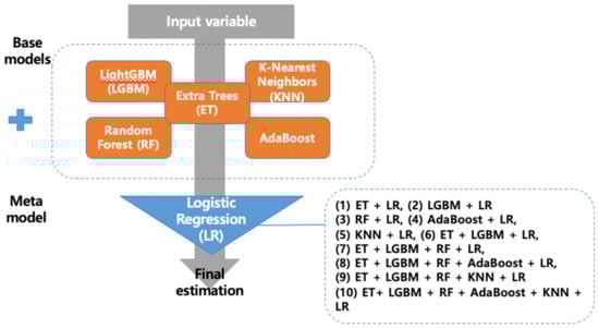
Figure 1.
Process flow diagram for predictive models.
2.6. Model Evaluation
Ten-fold cross-validation was applied to verify the prediction performance of the nine machine learning models that were built. In order to assess the prediction performance, this study employed the indices accuracy, precision, recall, and F1-score. The computation formula for each evaluation index is shown below:
Accuracy = (Truepositive + Truenegative)/(Truepositive + Truenegative + Falsepositive + Falsenegative)
Precision = Truepositive/(Truepositive + Falsepositive)
Recall = Truepositive/(Truepositive + Falsenegative)
F1 score = 2 * (Precision * Recall) * (Precision + Recall).
Our study used the assumption that a model with the highest F1-score has the best prediction ability. The model with the highest recall was regarded as the best model if the F1-score remained constant. Python 3.11.0 was used for all analyses (https://www.python.org, accessed on 23 November 2022).
2.7. Hyperparameters Fine-Tuning by Sckit-Optimize Library
Hyperparameter optimization is the process of conducting a search to identify the set of particular model configuration arguments that provide the model’s optimal performance on a given dataset. Although there are several approaches to hyperparameter optimization, contemporary techniques such as Bayesian Optimization are quick and efficient. An open-source Python library called Scikit-Optimize (version 0.8.1) offers a Bayesian optimization implementation that may be used to fine-tune the hyperparameters of machine learning models from the scikit-learn Python library.
2.8. Local Interpretable Model-Agnostic Explanations (LIME)
In order to explain the outcomes of a machine learning system, it is necessary to make a relationship between the inputs to the system and the outputs in a manner that people can understand. The topic has become increasingly relevant in recent years [23,24]. Modern machine learning systems use highly parametric designs that make it difficult to comprehend the models’ findings. In our study, Local Interpretable Model-Agnostic Explanations (LIME) were used to develop explanations for the model’s output, which indicated the correlation between depression and other variables.
To provide an explanation for each prediction made by a black-box model, Ribeiro et al. [25] introduced LIME, a perturbation-based technique for its concrete implementation using local surrogate models. By combining perturbed inputs and the appropriate black-box model outputs, this method creates a new dataset that is weighted around the instance under investigation. The extra data points are then given a weight based on the original data point by the algorithm. Finally, a surrogate model, such as linear regression, is fitted to the dataset using the sample weights. The trained explanation model may then be used to explain each raw data piece. Formally, we define an explanation as a model g ∈ G, where G is a class of potentially interpretable models. More precisely, we let Ω(g) represent a complexity metric. In classification, f(x) represents the probability (or binary indicator) that x belongs to a certain class. In order to determine the locality around x, we further use πx(z) as a closeness measure between an instance z to x. Let (f, g, πx) be a measure of how inaccurately g approximates f in the locale denoted by πx. We need to keep Ω(g) low enough to be interpretable by people while minimizing (f, g, πx) to guarantee local fidelity and interpretability. As a result of the following, LIME’s explanation is obtained: . This formulation can be used with different explanation families G, fidelity functions , and complexity measures Ω [25].
3. Results
3.1. Selected Features Assessment
In this study, REFCV selected features by using 5-fold cross-validation and accuracy as a measure-score. As a result, only 10 features were chosen from a total of 35 variables. REFCV features included DEM_AGE, DEM_EDU, DEM_ADPD_AGE, DEM_PD_DMCI_AGE, DEM_KMMSE_SCR, DEM_KMOCA_SCR, DEM_CDR_SSCR, DEM_KIADL_SCR, DEM_UPDRS_MSCR, and DEM_HYSTAG_SCR. When total variables were used, the base models were ranked in ordinal: LGBM, KNN, ET, RF, and AdaBoost. LGBM performed the best in this instance, with 0.7155 accuracy, 0.8045 recall, 0.7394 precision, and a 0.7658 F1-score. Meanwhile, for the features of REFCV, the ranking of the base models was slightly altered to LGBM, RF, ET, AdaBoost, and KNN. With accuracy, recall, precision, and F1-scores of 0.7400, 0.8199, 0.7606, and 0.7858, respectively, LGBM also demonstrated the best performance. The findings demonstrate that the REFCV feature selection method improved base models’ performance in this study dataset. Table 2 details the performance of the base models when using either all features or REFCV’s features.
Table 2.
Comparison with ML models.
3.2. Hyperparameters Tuned Models Comparison
To further boost model performance before stacking, we also fine-tuned the hyperparameters of each base model. By using Bayesian Optimization wrapped in the Scikit-Optimize library, the optimized model and its hyperparameters are shown below:
- LGBM: bagging_fraction = 0.8374829161718105, bagging_freq = 6, feature_fraction = 0.5841143936824905, learning_rate = 0.025450870095720408, min_child_samples = 2, min_split_gain = 0.1853520160149429, n_estimators = 234, num_leaves = 242, random_state = 3317, reg_alpha = 0.0032933153051456932, reg_lambda = 3.2851517043202704 × 10⁻⁶.
- RF: bootstrap = False, criterion = ‘entropy’, max_depth = 11, max_features = 0.4, min_impurity_decrease = 1 × 10⁻⁹, min_samples_leaf = 6, min_samples_split = 10, n_estimators = 300.
- ET: criterion = ‘entropy’, max_depth = 11, max_features = 1.0, min_impurity_decrease = 1.1410366199157523 × 10⁻⁷, min_samples_split = 3, n_estimators = 300.
- AdaBoost: learning_rate = 0.06748784395891723, n_estimators = 300.
- KNN: n_neighbors = 4, weights = ‘distance’.
After fine-tuning the hyper-parameters for each base model, the models’ performance increased significantly, and their rankings also changed. LGBM had the highest performance ranking among the base models, but after fine-tuning, it fell to second place, and ET became the model with the best performance. The ET model scored the best overall, with accuracy of 0.7690, recall of 0.8853, precision of 0.7672, and an F1-score of 0.8165. RF, AdaBoost, and KNN occupied the final three positions in the ranking order. Table 3 provides specifics on the performance of the hyperparameter fine-tuned models.
Table 3.
Performance of the hyperparameter fine-tuned models.
3.3. Comparing the Accuracy of Stacking Models Predicting the Depression of PWPD
Table 4 shows the predictive performance (accuracy, F1-score, precision, and recall) of 10 stacking models for predicting depression in PWPD, respectively. The results of our research indicated that the predictive performance of the “ET + LGBM + RF + LR” model (stacking ensemble: accuracy 0.7736, recall 0.8692, precision 0.7795, and F1-score 0.8172)” was the best compared with the best single model ET (accuracy 0.7690, recall 0.8853, precision 0.7672, and an F1-score 0.8165). Moreover, despite the stack model ET + LGBM + RF + AdaBoost + LR having the same performance as the top model, we did not select it. The explanation is that the model’s performance before adding AdaBoost was the same in models (8) and (10), in which AdaBoost is one of the base models. This indicates that the AdaBoost base model had no impact on the stacking ensemble models used to analyze the dataset in this study.
Table 4.
Performance of 10 stacking models.
3.4. Evaluation of LIME-Based Stacking Ensemble Model
We chose a specific instance to analyze in order to show how the LIME model works with the stacking ensemble model. Figure 2 depicts a description of a Parkinson’s disease patient suffering from depression. Figure 2a summarizes the patient’s state and contributing circumstances. This patient was 71 years old at that moment and was first diagnosed with PD at the age of 65 and with PD-D (Parkinson’s disease with dementia) or PD-MCI (Parkinson’s disease with mild cognitive impairment) at the age of 69. This person’s education period was 9 years. In addition, the patient had the Korean mini mental state examination score (DEM_KMMSE_SCR) at 25/30 points, the Clinical dementia rating sum of boxes (DEM_CDR_SSCR) at 4/5 points, the Korean montreal cognitive assessment (DEM_KMOCA_SCR) at 12/30 points, K-iADL(Korean instrumental activities of daily living score at 28 points, the Hoehn and Yahr staging score (DEM_HYSTAG_SCR) at 5/5 points, and the Motor Untitled Parkinson disease rating scale score (DEM_UPDRS_MSCR) at 45/108 points.
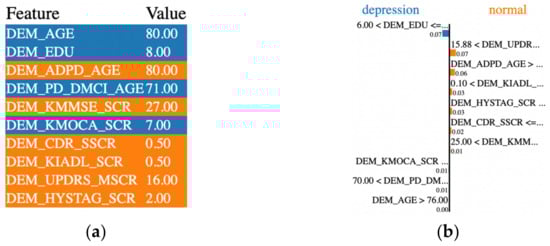
Figure 2.
Example of a PD patient with depression experience.
Our stacking ensemble model predicted that the patient would have severe depression with a probability of 85%. Figure 2b depicts the LIME methodology. The orange bars represent the variables that significantly contribute to the prediction’s rejection, whereas the blue bars represent the states and factors that considerably contribute to the prediction’s support. According to the explanation, at the time of the prediction, “the Motor Untitled Parkinson disease rating scale score, the Hoehn and Yahr staging score, K-iADL score, education period, first diagnosis age, the Korean montreal cognitive assessment, and the Korean mini mental state examination score” were the target’s main factors and states that most contribute to the prediction.
After applying LIME to all testing data in case a person had depression, we evaluated the relative contributions of variables to the prediction of depression in PWPD. With a weight of 10.36 + 0.02%, the Motor Untitled Parkinson disease rating scale score (DEM_UPDRS_MSCR) contributed the most to model prediction, while the Hoehn and Yahr staging score (DEM_HYSTAG_SCR) contributed 8.29 + 0.01%. The Korean mini mental state examination score (DEM_KMMSE_SCR), the Clinical dementia rating sum of boxes (DEM_CDR_SSCR), and the education period (DEM_EDU) were responsible for 6.82%, 5.05%, and 3.63% of the variance, respectively. As seen in Figure 3, the top variables for depression prediction were arranged in detail.
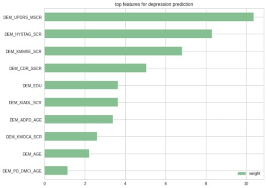
Figure 3.
LIME’s top features for depression prediction cases.
4. Discussion
This study compared the predictive performance of 15 machine learning algorithms to predict depression in PWPD in South Korea and confirmed that the ET + LGBM + RF + LR model had the best predictive performance. The findings were consistent with previous research [9,26,27], which found that the stacking ensemble model’s root-mean-square error (RMSE) was lower than that of the single machine learning model. Byeon (2021) [9] showed that the stacking ensemble model had a higher index of agreement, variance of errors, and accuracy than the single machine learning model, implying that its predictive performance could be higher for structured data such as examination data. Our research confirms this statement. Furthermore, Kaur et al. [27] demonstrated that even when all base models are combined, the stacking ensemble model does not always perform at its best. Our research also shows that combining three models into a total of five base models yielded the best performance; consequently, performance of a stacking ensemble model would be better when a model with harmony is selected rather than including all algorithms unconditionally.
Another finding of this study was the importance of the feature selection method to the model’s performance. The prediction outcomes of all models are stable once the number of chosen features exceeds a certain threshold, and adding more features will not only increase the models’ accuracy but will significantly increase the amount of computation. According to Zhang et al. [28], the REFCV feature selection method allowed them to outperform earlier studies with their Alzheimer’s disease prediction model. Our model was also reduced from 35 to 10 variables, thereby decreasing execution time and enhancing its performance. Our model’s performance was improved and execution time was lowered by reducing its 35 variables to 10. Moreover, reducing noise enables the hyperparameter to be fine-tuned with a broader range of values without excessive execution time, resulting in a more effective model.
The importance of this study is that we created a LIME-based stacking ensemble prediction model for depression in PWPD in order to explain the depression judgment of AI in a way that medical professionals can comprehend. Similar to the results of this study, many previous studies reported that the major risk factors for depression in Parkinson’s patients were gender, education level, early age at onset of PD, and age [29,30]. The fundamental processes of depression in PWPD remain unknown [31]. Nonetheless, previous studies discovered that women with PD were far more likely to be depressed. This is analogous to the general population’s gender bias in depression [32,33]. Future research is required to discover the relationship between demographic characteristics and depression in PWPD based on a large-scale cohort.
It is critical to stress to patients, their families, and other professionals that PWPD may be treated and that recovery is achievable. Unfortunately, depressive disorders are rarely recognized in professional settings, and even when they are, they are typically not adequately treated [34]. Even though depression is common in PWPD, only 1% of PWPD stated that they had depression, according to the Global Parkinson’s Disease Survey Steering Committee’s 2002 findings. These results show that, although PWPD regularly suffer depression, many PWPD, their careers, and their medical practitioners do not find depression symptoms or treat them as aging symptoms, and the patients do not receive proper diagnosis or therapy. Several studies [34,35,36] examining the risk factors for depression in PWPD have reported that daily living ability, sleep behavior disorders, cognitive level, Hoehn and Yahr stage, and environmental factors (such as social stigma and social involvement) are significant determinants of depression. These results corroborated the findings of selected factors used to develop our study’s predictive model.
The limitations of this study are as follows. First, although the model can be interpreted, the performance of our stacking ensemble model is lower than the support vector machine in Byeon [37]. Future studies are needed to find a more accurate model or explore more about features that should be used. Second, there was only a tiny sample size. Thirdly, causation could not be determined due to the cross-sectional nature of the study. To establish causality, further longitudinal research is necessary. Lastly, LIME’s explanations are not always stable or consistent due to the use of different samples or the definition of which local data points are included in the local model.
5. Conclusions
In conclusion, this study created a LIME-based stacking ensemble model to explain depression or non-depression predictions generated by a “black-box” deep learning model. The results offer a trustworthy stacking ensemble model that can aid PWPD in the prediction of depression. The LIME explanations show that this stacking ensemble model makes decisions similar to humans based on extremely logical factors. For “black-box” machine learning predictive technologies to be widely adopted in healthcare, more study into improving LIME and the traits that raise its trust among physicians is essential.
Author Contributions
Conceptualization, H.V.N. and H.B.; software, H.V.N.; methodology, H.V.N. and H.B.; validation, H.V.N. and H.B.; investigation, H.V.N. and H.B.; writing—original draft preparation, H.V.N.; formal analysis, H.B.; writing—review and editing, H.B.; visualization, H.V.N.; supervision, H.B.; project administration, H.B.; funding acquisition, H.B. All authors have read and agreed to the published version of the manuscript.
Funding
This research Supported by Basic Science Research Program through the National Research Foundation of Korea (NRF) funded by the Ministry of Education (NRF-2018R1D1A1B07041091, NRF-2021S1A5A8062526).
Institutional Review Board Statement
The study was carried out in accordance with the Helsinki Declaration and was approved by the Korea Workers’ Compensation and Welfare Service’s Institutional Review Board (or Ethics Committee) (protocol code 0439001, date of approval 31 January 2018).
Informed Consent Statement
Informed consent was obtained from all subjects involved in the study.
Data Availability Statement
The data presented in this study are provided at the request of the corresponding author. The data is not publicly available because researchers need to obtain permission from the Korea Centers for Disease Control and Prevention.
Conflicts of Interest
The authors declare no conflict of interest.
References
- Rossi, A.; Berger, K.; Chen, H.; Leslie, D.; Mailman, R.B.; Huang, X. Projection of the Prevalence of Parkinson’s Disease in the Coming Decades: Revisited. Mov. Disord. 2017, 33, 156–159. [Google Scholar] [CrossRef] [PubMed]
- Baek, J.Y.; Lee, E.; Jung, H.-W.; Jang, I.-Y. Geriatrics Fact Sheet in Korea 2021. Ann. Geriatr. Med. Res. 2021, 25, 65–71. [Google Scholar] [CrossRef] [PubMed]
- Reijnders, J.S.A.M.; Ehrt, U.; Weber, W.E.J.; Aarsland, D.; Leentjens, A.F.G. A Systematic Review of Prevalence Studies of Depression in Parkinson’s Disease. Mov. Disord. 2007, 23, 183–189. [Google Scholar] [CrossRef] [PubMed]
- Wichowicz, H.M.; Sławek, J.; Derejko, M.; Cubała, W.J. Factors Associated with Depression in Parkinson’s Disease: A Cross-Sectional Study in a Polish Population. Eur. Psychiatry 2006, 21, 516–520. [Google Scholar] [CrossRef]
- Global Parkinson’s Disease Survey Steering Committee. Factors Impacting on Quality of Life in Parkinson’s Disease: Results from an International Survey. Mov. Disord. 2002, 17, 60–67. [Google Scholar] [CrossRef]
- Byeon, H. Predicting the Severity of Parkinson’s Disease Dementia by Assessing the Neuropsychiatric Symptoms with an SVM Regression Model. Int. J. Environ. Res. Public Health 2021, 18, 2551. [Google Scholar] [CrossRef]
- Avuçlu, E.; Elen, A. Evaluation of Train and Test Performance of Machine Learning Algorithms and Parkinson Diagnosis with Statistical Measurements. Med. Biol. Eng. Comput. 2020, 58, 2775–2788. [Google Scholar] [CrossRef]
- Byeon, H. Comparing Ensemble-Based Machine Learning Classifiers Developed for Distinguishing Hypokinetic Dysarthria from Presbyphonia. Appl. Sci. 2021, 11, 2235. [Google Scholar] [CrossRef]
- Byeon, H. Exploring Factors Associated with the Social Discrimination Experience of Children from Multicultural Families in South Korea by Using Stacking with Non-Linear Algorithm. Int. J. Adv. Comput. Sci. Appl. 2021, 12, 125–130. [Google Scholar] [CrossRef]
- Byeon, H. Can the Prediction Model Using Regression with Optimal Scale Improve the Power to Predict the Parkinson’s Dementia? World J. Psychiatry 2022, 12, 1031–1043. [Google Scholar] [CrossRef]
- Albreiki, B.; Zaki, N.; Alashwal, H. A Systematic Literature Review of Student’ Performance Prediction Using Machine Learning Techniques. Educ. Sci. 2021, 11, 552. [Google Scholar] [CrossRef]
- Mutlag, W.K.; Ali, S.K.; Aydam, Z.M.; Taher, B.H. Feature Extraction Methods: A Review. J. Phys. Conf. Ser. 2020, 1591, 012028. [Google Scholar] [CrossRef]
- Cawley, G.C.; Nicola, L.C. Talbot. On Over-fitting in Model Selection and Subsequent Selection Bias in Performance Evaluation. J. Mach. Learn. Res. 2010, 11, 2079–2107. [Google Scholar]
- Kuhn, M.; Johnson, K. Feature Engineering and Selection; Chapman and Hall/CRC Data Science Ser.; Chapman & Hall/CRC: Boca Raton, FL, USA, 2019; ISBN 978-1-315-10823-0. [Google Scholar]
- Friedman, J.H. Greedy Function Approximation: A Gradient Boosting Machine. Ann. Stat. 2001, 29, 1189–1232. [Google Scholar] [CrossRef]
- Ke, G.; Meng, Q.; Finley, T.; Wang, T.; Chen, W.; Ma, W.; Ye, Q.; Liu, T.Y. LightGBM: A Highly Efficient Gradient Boosting Decision Tree. In Proceedings of the 31st Conference on Neural Information Processing Systems (NIPS 2017), Long Beach, CA, USA, 4–9 December 2017; Volume 30. [Google Scholar]
- Breiman, L. Random Forest. Mach. Learn. 2001, 45, 5–32. [Google Scholar] [CrossRef]
- Svetnik, V.; Liaw, A.; Tong, C.; Culberson, J.C.; Sheridan, R.P.; Feuston, B.P. Random Forest: A Classification and Regression Tool for Compound Classification and QSAR Modeling. J. Chem. Inf. Comput. Sci. 2003, 43, 1947–1958. [Google Scholar] [CrossRef]
- GALTON, F. Vox Populi. Nature 1907, 75, 450–451. [Google Scholar] [CrossRef]
- Geurts, P.; Ernst, D.; Wehenkel, L. Extremely Randomized Trees. Mach. Learn. 2006, 63, 3–42. [Google Scholar] [CrossRef]
- Dezhen, Z.; Kai, Y. Genetic Algorithm Based Optimization for AdaBoost. In Proceedings of the 2008 International Conference on Computer Science and Software Engineering, Wuhan, China, 12–14 December 2008. [Google Scholar] [CrossRef]
- Kleinbaum, D.G.; Klein, M. Logistic Regression; Statistics for Biology and Health Ser.; Springer: Berlin/Heidelberg, Germany, 2010; ISBN 978-1-4419-1742-3. [Google Scholar]
- Roscher, R.; Bohn, B.; Duarte, M.F.; Garcke, J. Explainable Machine Learning for Scientific Insights and Discoveries. IEEE Access 2020, 8, 42200–42216. [Google Scholar] [CrossRef]
- Nguyen, H.V.; Byeon, H. Explainable Deep-Learning-Based Depression Modeling of Elderly Community after COVID-19 Pandemic. Mathematics 2022, 10, 4408. [Google Scholar] [CrossRef]
- Ribeiro, M.T.; Singh, S.; Guestrin, C. Why should I trust you? Explaining the predictions of any classifier. In Proceedings of the 22nd ACM SIGKDD International Conference on Knowledge Discovery and Data Mining, San Francisco, CA, USA, 13–17 August 2016; pp. 1135–1144. [Google Scholar]
- Yadav, D.C.; Pal, S. To Generate an Ensemble Model for Women Thyroid Prediction Using Data Mining Techniques. Asian Pac. J. Cancer Prev. 2019, 20, 1275–1281. [Google Scholar] [CrossRef] [PubMed]
- Kaur, H.; Poon, P.K.-C.; Wang, S.Y.; Woodbridge, D.M. Depression Level Prediction in People with Parkinson’s Disease during the COVID-19 Pandemic. In Proceedings of the 2021 43rd Annual International Conference of the IEEE Engineering in Medicine & Biology Society (EMBC), Mexico, 1–5 November 2021. [Google Scholar] [CrossRef]
- Zhang, F.; Petersen, M.; Johnson, L.; Hall, J.; O’Bryant, S.E. Recursive Support Vector Machine Biomarker Selection for Alzheimer’s Disease. J. Alzheimer’s Dis. 2021, 79, 1691–1700. [Google Scholar] [CrossRef] [PubMed]
- Perrin, A.J.; Nosova, E.; Co, K.; Book, A.; Iu, O.; Silva, V.; Thompson, C.; McKeown, M.J.; Stoessl, A.J.; Farrer, M.J.; et al. Gender Differences in Parkinson’s Disease Depression. Parkinsonism Relat. Disord. 2017, 36, 93–97. [Google Scholar] [CrossRef]
- Cummings, J.L. Depression and Parkinson’s Disease: A Review. Am. J. Psychiatry 1992, 149, 443–454. [Google Scholar] [CrossRef] [PubMed]
- Marsh, L. Depression and Parkinson’s Disease: Current Knowledge. Curr. Neurol. Neurosci. Rep. 2013, 13, 409. [Google Scholar] [CrossRef]
- Riedel, O.; Heuser, I.; Klotsche, J.; Dodel, R.; Wittchen, H.U.; GEPAD Study Group. Occurrence Risk and Structure of Depression in Parkinson Disease with and without Dementia: Results from the GEPAD Study. J. Geriatr. Psychiatry Neurol. 2009, 23, 27–34. [Google Scholar] [CrossRef]
- Aarsland, D.; Påhlhagen, S.; Ballard, C.G.; Ehrt, U.; Svenningsson, P. Depression in Parkinson Disease—Epidemiology, Mechanisms and Management. Nat. Rev. Neurol. 2011, 8, 35–47. [Google Scholar] [CrossRef]
- Dobkin, R.D.; Rubino, J.T.; Friedman, J.; Allen, L.A.; Gara, M.A.; Menza, M. Barriers to Mental Health Care Utilization in Parkinson’s Disease. J. Geriatr. Psychiatry Neurol. 2013, 26, 105–116. [Google Scholar] [CrossRef]
- Havlikova, E.; van Dijk, J.P.; Nagyova, I.; Rosenberger, J.; Middel, B.; Dubayova, T.; Gdovinova, Z.; Groothoff, J.W. The Impact of Sleep and Mood Disorders on Quality of Life in Parkinson’s Disease Patients. J. Neurol. 2011, 258, 2222–2229. [Google Scholar] [CrossRef]
- Lawrence, B.J.; Gasson, N.; Kane, R.; Bucks, R.S.; Loftus, A.M. Activities of Daily Living, Depression, and Quality of Life in Parkinson’s Disease. PLoS ONE 2014, 9, e102294. [Google Scholar] [CrossRef]
- Byeon, H. Development of a Depression in Parkinson’s Disease Prediction Model Using Machine Learning. World J. Psychiatry 2020, 10, 234–244. [Google Scholar] [CrossRef]


Disclaimer/Publisher’s Note: The statements, opinions and data contained in all publications are solely those of the individual author(s) and contributor(s) and not of MDPI and/or the editor(s). MDPI and/or the editor(s) disclaim responsibility for any injury to people or property resulting from any ideas, methods, instructions or products referred to in the content. |
© 2023 by the authors. Licensee MDPI, Basel, Switzerland. This article is an open access article distributed under the terms and conditions of the Creative Commons Attribution (CC BY) license (https://creativecommons.org/licenses/by/4.0/).