AdvSCOD: Bayesian-Based Out-Of-Distribution Detection via Curvature Sketching and Adversarial Sample Enrichment

Abstract

Detecting out-of-distribution (OOD) samples is critical for the deployment of deep neural networks (DNN) in real-world scenarios. An appealing direction in which to conduct OOD detection is to measure the epistemic uncertainty in DNNs using the Bayesian model, since it is much more explainable. SCOD sketches the curvature of DNN classifiers based on Bayesian posterior estimation and decomposes the OOD measurement into the uncertainty of the model parameters and the influence of input samples on the DNN models. However, since lots of approximation is applied, and the influence of the input samples on DNN models can be hardly measured stably, as demonstrated in adversarial attacks, the detection is not robust. In this paper, we propose a novel AdvSCOD framework that enriches the input sample with a small set of its neighborhoods generated by applying adversarial perturbation, which we believe can better reflect the influence on model predictions, and then we average their uncertainties, measured by SCOD. Extensive experiments with different settings of in-distribution and OOD datasets validate the effectiveness of AdvSCOD in OOD detection and its superiority to state-of-the-art Bayesian-based methods. We also evaluate the influence of different types of perturbation.

1. Introduction

Deep neural networks (DNNs) [1,2,3,4] have revolutionized the solution of a variety of computer vision tasks, e.g., image classification and semantic segmentation, and they have refreshed the state-of-the-art records. However, since these DNN models are designed under the closed-world assumption [5], they can be hardly deployed in real-world scenarios directly. One of the major obstacles is the out-of-distribution (OOD) samples that inevitably exist. Indeed, many recent studies have reported that DNN models make overconfident predictions on OOD samples [6] and thus have hidden risks in terms of safety issues.

Current solutions to deal with OOD overconfidence issues can be broadly divided into two categories. One branch of research focuses on alleviating the issue by suppressing the prediction confidences on a small set of typical OOD samples [7,8]. However, since the suppression on this typical set can hardly generalize to all OOD samples, the OOD overconfidence issue still exists. The other branch of research instead conducts pre-step OOD detection, and thus can reject OOD samples before feeding them to the DNN models.

To conduct OOD detection, many OOD scores that show how likely a sample is to be OOD have been recently devised. Hendrycks et al. [9] proposed utilizing probabilities from softmax distributions of DNN classifiers. Though simple, this solution is validated as often being sufficient for OOD detection. Later, researchers have investigated the improvement of OOD detection by utilizing temperature scaling and adding small perturbations [10], Mahalanobis distance [11], energy-based models [12], logit normalization [13], etc. Although good detection performance has been shown, it is hardly explainable how this is attributable to these OOD scores.

An orthogonal yet more appealing direction is to employ Bayesian models to reformulate the problem [14], since it is much more explainable to some extent. The rationale behind this direction is that the uncertainty of input samples, i.e., the likelihood of being OOD, is usually highly related to the uncertainty of DNN parameters, which can be measured by Bayesian approximation. 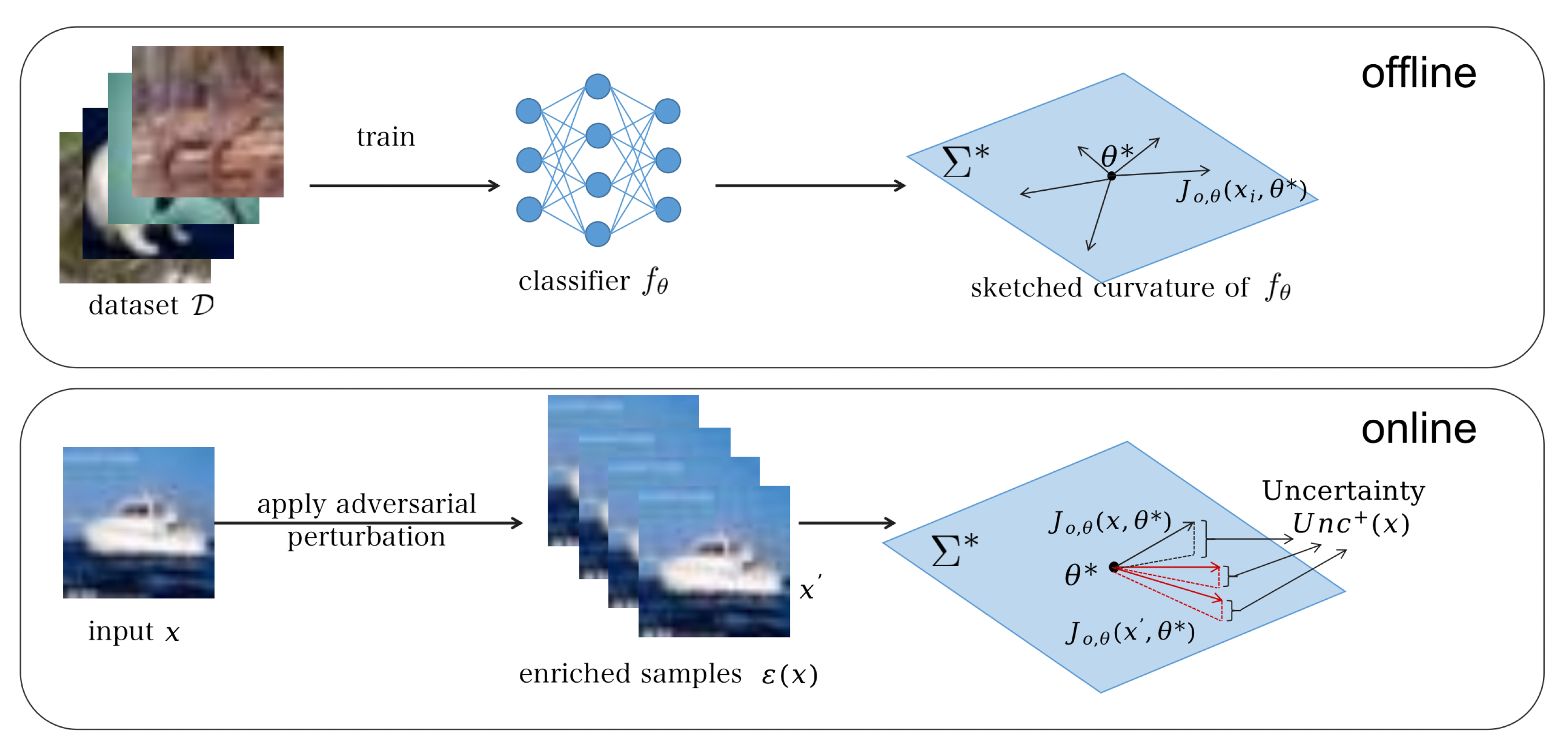Recently, sketching curvature for OOD detection (SCOD) [15] makes it efficient and effective by using the local sketched curvature (Hessian/Fisher) of DNN models as a bridge. Specifically, they measure the final uncertainty based on both the uncertainty of the model parameters and the influence of input samples on the DNN models. In particular, however, since a plethora of approximations is applied in the process, and the influence of an input sample on DNN models can hardly be estimated stably, we observe that there are deviations in the estimated uncertainty for a certain number of input samples.

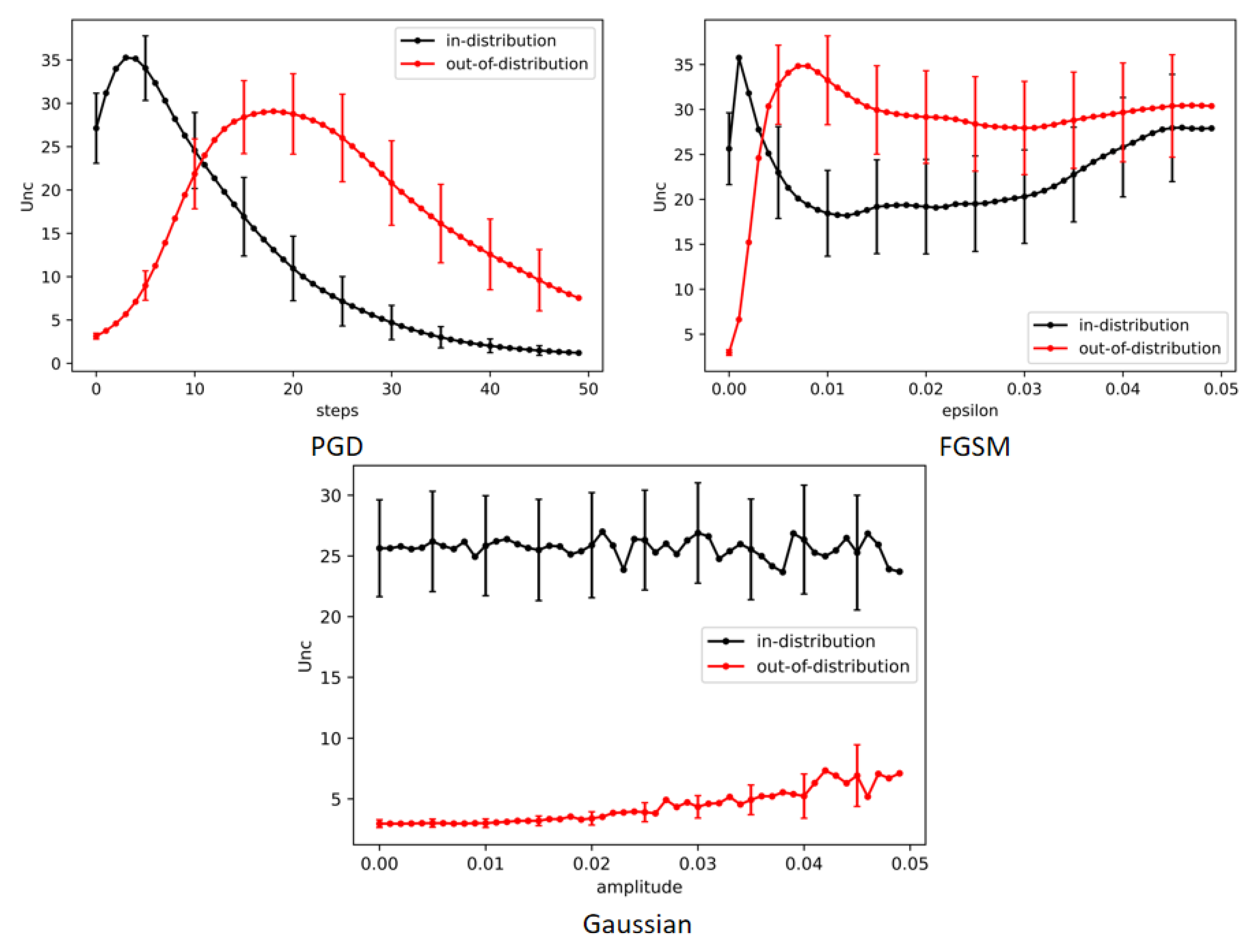
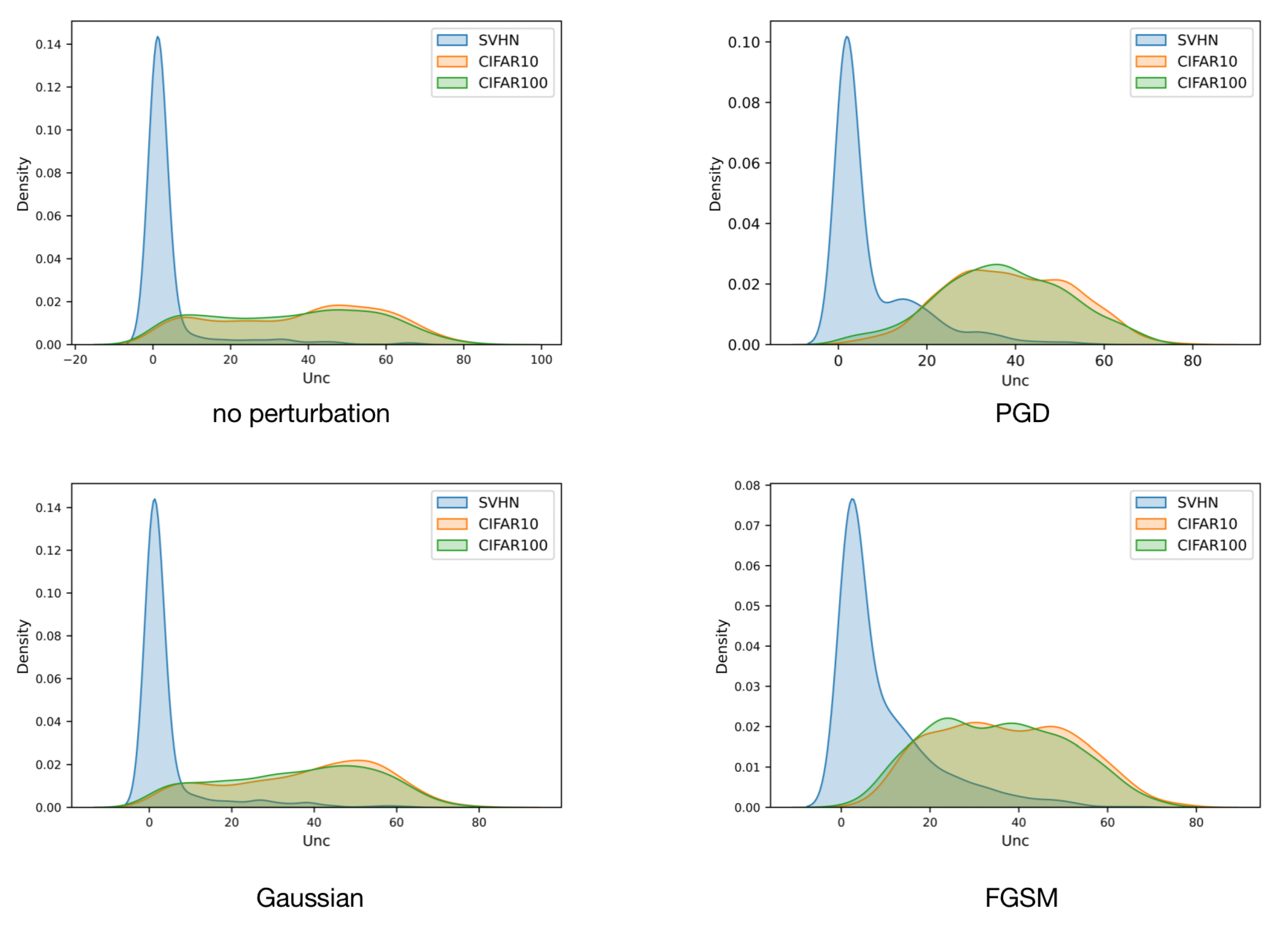
To resolve the above issue, we propose a novel AdvSCOD framework that estimates the uncertainty for each input sample by aggregating that of a small set of samples in its neighborhood. In particular, inspired by the fact that adversarial attacks that show imperceptible perturbation can lead DNN models to make totally different predictions, we enrich the input sample by applying adversarial perturbation to it, which we believe will better reflect the influence of the input sample on DNN models. Extensive experiments validate how our proposed AdvSCOD outperforms the state-of-the-art Bayesian-based methods on OOD detection. Furthermore, we also experimentally demonstrate that adversarial perturbation is better than several other types of perturbation.

Overall, our key contributions are summarized as follows:

• We propose a novel AdvSCOD framework that estimates the uncertainty of each input sample by aggregating its small neighborhoods.
• We conduct extensive experiments to validate the effectiveness of AdvSCOD and its superiority to state-of-the-art Bayesian-based OOD detection methods.
• We provide a new perspective on evaluating the sample’s influence on DNN models in view of adversarial attacks.

2. Related Work

2.1. OOD Detection

The most common solution for handling the OOD overconfidence issue of DNN models [7] is to conduct OOD detection, i.e., detecting and then rejecting OOD inputs. According to the presence or absence of label information, existing OOD detection approaches can be broadly divided into two categories: generative-based and discriminative-based.

Generative-based methods aim to model the distribution of the training dataset, e.g., by using auto-encoder [16], flow-based models [17], and autoregressive models [18,19], and thus the estimation of the likelihood of given inputs can be measured by distribution shift. Indeed, it is intuitive that the likelihood of the in-distribution (ID) samples should be higher than that of the OOD samples. However, since current generative models tend to overfit the training set, many recent works show that they are not robust in OOD detection [20]. Discriminative-based methods instead conduct OOD detection utilizing the label information. Hendrycks et al. [9] observed that using the simple maximum softmax probabilities (MSP) of DNN classifiers is sufficient for differentiating ID and OOD samples. Later, researchers further improved OOD detection by utilizing temperature scaling and adding small perturbations [10], Mahalanobis distance [11], energy-based models [12,21,22,23,24], logit normalization [13], etc. For a more complete review of OOD detection, please refer to the survey paper [25]. Different from what has been thoroughly explored, we investigate in an orthogonal direction, i.e., by employing Bayesian models.

2.2. Bayesian-Based OOD Detection

Since Bayesian approximation is powerful in characterizing epistemic uncertainty in DNNs, it is promising in handling the OOD detection task. However, Bayesian methods traditionally rely on Monte Carlo [26] or variational inference [27,28,29] and thus are not suitable for pre-trained DNNs. Therefore, current researchers instead apply the Laplace approximation to the Bayesian posterior [30], even though it requires estimating the curvature of DNNs, which is very time-consuming. Sketching curvature for OOD detection (SCOD) [15] uses the Fisher information matrix to approximate the Hessian matrix, making the process efficient. Instead of calculating the uncertainty of DNNs with a single input sample as in SCOD, we further enrich it by applying adversarial perturbations and thus making the estimation more robust.

2.3. Sample Enrichment and Adversarial Attack

Sample enrichment, or data augmentation, is widely adopted for preventing DNN models from overfitting by synthesizing label-preserving images [31,32]. It can be realized by applying random crop, padding, flipping, rotating, scaling, etc. Another type of sample enrichment adds adversarial perturbation to the training images, aiming at improving the adversarial robustness [33]. We leverage the idea of adversarial perturbation to achieve sample enrichment, which aims to make the estimation of uncertainty more accurate.

Another related direction to ours is adversarial attack [33,34,35,36,37,38], whose purpose is to apply imperceptible perturbation to mislead DNN classifiers. In contrast, we apply adversarial perturbation to the input sample to enrich it for better evaluating the influence on the DNN models.

3. Background and Problem Formulation

3.1. Problem Statement of OOD Detection

We formulate the problem in the context of image classification with DNNs. Given a DNN classifier $f_{\theta }$ trained on the dataset $\mathcal{D}$ with pairs of images and their corresponding labels $\{(x_i,y_i)\mid i=1,\dots ,M\}$, where $x_i\in R^d$ and $y_i\in \{1,2,\dots ,K\}$ and $\theta$ represents the parameters of f, we aim to define a measurement that can determine whether an input image $x\in R^d$ belongs to the ID or OOD samples by using $f_{\theta }$.

3.2. Bayesian Neural Networks and OOD Detection

Probabilistic DNN. The DNN classifier $f_{\theta }$ can be considered as a probabilistic model $P(y\mid x,\theta )$. Given an input image x, the classifier f outputs o using weights $\theta$,

$$o=f_{\theta }\left(x\right),$$

(1)

where o is the predicted logit, and then a distributional family $\mathcal{P}$ maps o to a distribution over the targets, i.e., $P\left(y\right)$,

$$P\left(y\right)=\mathcal{P}\left(o\right)$$

(2)

In this view, we can learn the weights $\theta$ by maximum likelihood (MLE) estimation,

$$\begin{array}{cc}\hfill {\theta }^{\mathrm{MLE}}& =arg\underset{\theta }{max}logP(\mathcal{D}\mid \theta )\hfill \\ \hfill & =arg\underset{\theta }{max}\sum logP\left(y_i\mid x_i,\theta \right)\hfill \end{array}$$

(3)

By giving a prior of $\theta$, it further becomes a maximum posterior estimate (MAP),

$$\begin{array}{cc}\hfill {\theta }^{\mathrm{MAP}}& =arg\underset{\theta }{max}logP(\theta \mid \mathcal{D})\hfill \\ \hfill & =arg\underset{\theta }{max}logP(\mathcal{D}\mid \theta )+logP\left(\theta \right)\hfill \end{array}$$

(4)

Bayesian Neural Networks. Instead of estimating a single optimal point as in Equation (4), Bayesian neural networks (BNN) find the posterior distribution $P(\theta \mid \mathcal{D})$ of the parameter $\theta$ and thus introduce uncertainty in the prediction.

Formally, the predictive distribution of an unknown label y of a test data item x is given by

$$P(y\mid x)={\mathbb{E}}_{P(\theta \mid \mathcal{D})}\left[P(y\mid x,\theta )\right]$$

(5)

However, directly calculating the above equation is usually intractable. Therefore, researchers usually use Laplace approximation to estimate the distribution $P(\theta \mid \mathcal{D})$ and use Monte Carlo sampling to calculate the final expected value.

BNN-based OOD Detection. Many recent works show that the uncertainty of BNN can be utilized for OOD detection, since the predictions on ID and OOD samples have different uncertainties [39,40,41,42,43].

Suppose the prior of $\theta$ follows a Gaussian distribution with a standard deviation of $\sigma$; the Laplace posterior of the variance of $\theta$ can be calculated by

$$\mathsf{\Sigma }=\frac{1}{2}{(H_L+\frac{1}{2{\sigma }^{2}I})}^{-1}$$

(6)

where $H_L$ is the Hessian matrix with respect to the parameters of the pretrained DNN classifier f, i.e., $\theta$, and I is an identity matrix. Therefore, we could utilize $\mathsf{\Sigma }$ to measure the uncertainty of DNNs, so as to conduct OOD detection [23,44].

However, for complex DNN models, calculating this exact Bayesian posterior approximation can still be challenging, where estimating and inversing huge matrices to calculate $\sigma$ is demanded.

3.3. SCOD [15]

The framework of sketching curvature for OOD Detection (SCOD) estimates the uncertainty in two respects: (1) the uncertainty of the model parameters on the prediction and (2) the influence of input samples on the DNN models.

For the uncertainty of the model parameters, SCOD re-estimates the variance of parameters by replacing the Hessian matrix in Equation (6) with the Fisher information matrix, whose calculation is more efficient and numerically stable,

$${\mathsf{\Sigma }}^{*}=\frac{1}{2}{\left(\sum _1^M{F}_{{\theta }^{*}}\left(x_i\right)+\frac{1}{2{\epsilon }^2}I\right)}^{-1},$$

(7)

where $F_{{\theta }^{*}}\left(x_i\right)$ denotes the weight-space Fisher evaluated for a particular input $x_i$ and the trained weights ${\theta }^{*}$, which is calculated by

$$F_{{\theta }^{*}}\left(x_i\right)=J_{o,{\theta }^{*}}^{\top }{F}_o\left(o\right)J_{o,{\theta }^{*}},$$

(8)

with $J_{o,{\theta }^{*}}$ denoting the Jacobian matrix evaluated for data $x_i$ under the parameter ${\theta }^{*}$. That is, $J_{o,{\theta }^{*}}[i,j]=\partial f_i/\partial {\theta }_j^{*}$. Note that the process of estimating the uncertainty can be conducted offline.

As for the influence of input samples, i.e., the uncertainty determined by the certain input sample x, we directly measure it using Equation (8), that is, $F_{\theta }^{*}\left(x\right)$. Note that this process is conducted online.

Therefore, the final uncertainty can be calculated as follows,

$$Unc\left(x\right)=Tr\left(F_{{\theta }^{*}}{\mathsf{\Sigma }}^{*}\right),$$

(9)

where $Tr(·)$ calculates the trace. Note that, although the calculation of Hessian matrix is much more efficient than the original Fisher matrix, SCOD further accelerates the process by splitting the original matrix into smaller ones. Since it is not the focus of this paper, we refer the reader to the original SCOD paper [15].

Discussion and Our Solution However, since lots of information is discarded in the approximation, the calculated Fisher information matrix may not be that accurate. Furthermore, as reported in the field of adversarial attacks, a slight change in the input image can lead the classifier to make a totally different prediction. In that case, the estimation of $J_{o,{\theta }^{*}}$ is also quite unstable. Both factors make the calculated uncertainty inaccurate.

To handle the above issues, we propose utilizing the averaged uncertainty calculated together with an enriched sample set in its small neighborhood, instead of using the value evaluated on a single one. In particular, since applying an adversarial attack is expected to bring about the largest deviation in $J_{o,{\theta }^{*}}$, we choose the enriched sample set obtained by applying adversarial perturbation.

4. Method

In this section, we propose a simple OOD detection framework with sketching curvature and adversarial sample enrichment (AdvSCOD). The framework consists of two key steps: sample enrichment via adversarial perturbation, and uncertainty averaging with enriched samples. Please refer to Figure 1 and Algorithm 1 for demonstration.

Algorithm 1 AdvSCOD

1: Input: $f_{\theta }(·);$▹ A pre-trained DNN model 2: $Unc(·);$▹ A SCOD function to calculate Uncertainty 3: x $;$▹ The input sample 4: $\lambda ,T,\alpha ;$ ▹ Hyperparameters 5: Output: ${Unc}^{+}$▹ An enhanced Unc value for input x 6: $x^0=x$; 7: for $t\leftarrow 1$ to T do 8:  $x^{t+1}={\mathsf{\Pi }}_{x+\mathcal{S}}\left(x^t+\alpha sgn\left({\mathcal{\nabla }}_{x}L(\theta ,x,y)\right)\right);$▹ PGD attack 9:  $\mathcal{E}\left(x\right).append\left(x^{t+1}\right)$; 10: end for 11: ${Unc}^{+}\left(x\right)=Unc\left(x\right)+\lambda \times {\sum }_{x^{{}^{\prime }}\in \mathcal{E}\left(x\right)}Unc\left(x^{{}^{\prime }}\right)$; 12: return${Unc}^{+}\left(x\right)$

4.1. Sample Enrichment via Adversarial Perturbation

To enrich the input sample x, we propose applying adversarial perturbation on x, which is imperceptible for humans, and thus will not introduce any semantic shifts. That is, the samples after applying perturbation have the same ID/OOD property as the original input sample x. Specifically, we choose the popular iterative-based projected gradient descent (PGD) [33],

$$x^{t+1}=Cli{p}_{x,ϵ}\left({\mathsf{\Pi }}_{x+\mathcal{S}}\left(x^t+\alpha sign\left({\mathcal{\nabla }}_{x}L(\theta ,x,y)\right)\right)\right)$$

(10)

where y is the predicted category made by the DNN classifier $f_{\theta }$ on the sample x, $L(\theta ,x,y)$ is the loss function, i.e., cross-entropy loss, for $f_{\theta }$, $\mathcal{S}\in R^d$ is the manipulative power of the adversary defined by a $l_{\infty }$-ball with radius $ϵ$, t is the iteration, $\alpha$ is the step size, and $sign(·)$ is the direction function.

Therefore, after T iterations of PGD, we finally obtain an enriched sample set $\mathcal{E}\left(x\right)=\{x^1,\dots ,x^T\}$.

4.2. Uncertainty Averaging with Enriched Samples

Given x and the enriched sample set $\mathcal{E}\left(x\right)=\{x^1,\dots ,x^T\}$, we calculate the final uncertainty simply by averaging the Unc value measured by SCOD,

$${Unc}^{+}\left(x\right)=Unc\left(x\right)+\lambda \times \sum _{x^{{}^{\prime }}\in \mathcal{E}\left(x\right)}Unc\left(x^{{}^{\prime }}\right)$$

(11)

where $\lambda$ is a hyperparameter that is empirically set to 0.01.

5. Experimental Results

5.1. Implementation

We implement our AdvSCOD framework and reproduce all the OOD detection methods mentioned above with PyTorch and report the results executed on a workstation with an Intel Xeon E5-2678 [email protected] Hz and 64 GB of memory using a single RTX 2080Ti GPU. For AdvSCOD, we set the number of adversarial samples $T=25$. For other OOD detection methods, we follow the settings in their original papers.

5.2. Experimental Setup

5.2.1. DNN Classifier and Datasets

For the DNN classifiers, we choose the popular GoogLeNet [45] on the datasets with color images, e.g., CIFAR-10, CIFAR-100, and SVHN, and LeNet [46] on the datasets with gray images, e.g., MNIST and Fashion. We convert color images to gray images, when evaluating using LeNet, and vice versa.

5.2.2. Perturbation Solutions

We adopted three perturbation methods, including two adversarial perturbations, i.e., PGD [33] and FGSM [47], and one Gaussian perturbation. FGSM is a one-step adversarial attack method by which we generate a series of perturbated samples via adjusting the amplitude. For PGD, we consider all the intermediate samples generated during the attack as perturbated samples. For the Gaussian perturbation, we collected perturbated samples by applying different intensities of Gaussian noise. Specifically, we set $\alpha =0.0002,l_{\infty }$ bound $ϵ=0.01$ in PGD perturbation for the experiments on SVHN, CIFAR10, and CIFAR100, and $\alpha =0.002,ϵ=0.1$ for the experiments on MNIST and Fashion. For the perturbation amplitude in FGSM and Gaussian perturbation, we set the range between 0 and $0.05$ on SVHN, CIFAR10, and CIFAR100, and we set the range between 0 and $0.2$ for MNIST and Fashion. The mean and variance of Gaussian perturbation are set to 0 and 1, respectively.

5.2.3. Baseline OOD Detection Solutions

We compared our proposed AdvSCOD with four state-of-the-art Bayesian-based OOD detection solutions, i.e., Naive [40], KFAC Laplace [48], Local Ensembles [44], and SCOD [15]. Naive produces a measure of uncertainty directly from the output of the pretrained model. The KFAC Laplace and Local Ensembles are similar to ours, with both using the curvature of the model to enhance the pretrained model for uncertainty estimation. Even though KFAC Laplace also relies on Laplace approximation, it uses different approximation methods to approximate the results of the Hessian matrix. Local Ensembles instead uses local second-order information to approximate the variance of prediction results across an ensemble of models from the same class.

5.2.4. Evaluation Metrics

To evaluate the performance of OOD detection, we adopted two commonly used metrics: AUROC and FPR95 following [9]. AUROC represents the area under the precise recall curve, and a larger value of the AUROC indicates better OOD detection performance. FPR95 represents the false positive rate of OOD examples when true positive rate of in-distribution examples is at 95%, which is better with lower values. Specifically, since better AUROC and FPR95 results are obtained if the OOD dataset has higher complexity than the ID one, we also adopted two other metrics, i.e., AUROC${}_{avg}$ and FPR95${}_{avg}$, which are the average values of AUROC and FRP95 with flipped settings of ID and OOD.

5.3. Performance Comparison and Analysis

5.3.1. Comparison of Our Results with The State-Of-The-Art Methods

We compare AdvSCOD with three state-of-the-art Bayesian-based OOD detection solutions, i.e., Local Ensembles, KFAC Laplace, Naive, and SCOD. The results reported in

Table 1. Comparison of the OOD detection performance measured by AUROC (larger values are better). Bold numbers are superior results.

ID	OOD	Local Ensembles	KFAC Laplace	Naive	SCOD	AdvSCOD
SVHN	CIFAR10	0.9371	0.9483	0.9480	0.9573	0.9668
	CIFAR100	0.9423	0.9462	0.9461	0.9456	0.9538
	MNIST	0.7379	0.7831	0.7910	0.7769	0.7568
	Fashion	0.9364	0.9426	0.9375	0.9391	0.9441
CIFAR10	SVHN	0.9198	0.9230	0.9235	0.9224	0.9358
	CIFAR100	0.8766	0.8788	0.8787	0.8768	0.8830
	MNIST	0.8727	0.8631	0.8747	0.8660	0.9281
	Fashion	0.9371	0.8634	0.8740	0.9106	0.9473
CIFAR100	SVHN	0.8047	0.8102	0.7779	0.8224	0.8323
	CIFAR10	0.7951	0.8115	0.7725	0.8071	0.8136
	MNIST	0.7086	0.7403	0.7111	0.7356	0.7512
	Fashion	0.8884	0.9226	0.9003	0.9179	0.9208
MNIST	SVHN	0.9601	0.9454	0.9796	0.9798	0.9870
	CIFAR10	0.9575	0.9459	0.9595	0.9767	0.9861
	CIFAR100	0.9692	0.9634	0.9685	0.9830	0.9900
	Fashion	0.9417	0.9373	0.9375	0.9554	0.9714
Fashion	SVHN	0.9673	0.9654	0.9941	0.9768	0.9790
	CIFAR10	0.9575	0.9459	0.9707	0.9810	0.9840
	CIFAR100	0.9692	0.9806	0.9739	0.9790	0.9824
	MNIST	0.8056	0.8347	0.7824	0.8876	0.9696

,

Table 2. Comparison of the OOD detection performance measured by AUROC${}_{avg}$. Bold numbers are superior results.

Dataset Pair	Local Ensembles	KFAC Laplace	Naive	SCOD	AdvSCOD
(SVHN,CIFAR10)	0.9284	0.9357	0.9357	0.9399	0.9513
(SVHN,CIFAR100)	0.8735	0.8782	0.8620	0.8840	0.8931
(SVHN,MNIST)	0.8490	0.8642	0.8853	0.8783	0.8719
(SVHN,Fashion)	0.9519	0.9540	0.9658	0.9580	0.9616
(CIFAR10,CIFAR100)	0.8358	0.8452	0.8256	0.8419	0.8483
(CIFAR10,MNIST)	0.9151	0.9045	0.9171	0.9214	0.9571
(CIFAR10,Fashion)	0.9473	0.9046	0.9224	0.9458	0.9657
(CIFAR100,MNIST)	0.8389	0.8518	0.8398	0.8593	0.8706
(CIFAR100,Fashion)	0.9288	0.9516	0.9371	0.9485	0.9516
(MNIST,Fashion)	0.8737	0.8860	0.8599	0.9215	0.9705

,

Table 3. Comparison of the OOD detection performance measured by FPR95 (lower value is better). Bold numbers are superior results.

ID	OOD	Local Ensembles	KFAC Laplace	Naive	SCOD	AdvSCOD
SVHN	CIFAR10	0.1872	0.1923	0.1928	0.1464	0.1417
	CIFAR100	0.1992	0.1952	0.1957	0.1682	0.1596
	MNIST	0.8037	0.8011	0.7056	0.7774	0.7941
	Fashion	0.2723	0.2184	0.2685	0.2604	0.1841
CIFAR10	SVHN	0.2278	0.2360	0.2348	0.2261	0.2221
	CIFAR100	0.3905	0.3896	0.3914	0.3846	0.3706
	MNIST	0.4282	0.4181	0.3875	0.4213	0.2633
	Fashion	0.4085	0.4181	0.3895	0.2735	0.1867
CIFAR100	SVHN	0.6118	0.5980	0.6206	0.5233	0.4872
	CIFAR10	0.5766	0.5742	0.6313	0.5518	0.5039
	MNIST	0.6206	0.6218	0.6566	0.6296	0.6034
	Fashion	0.4374	0.2936	0.3653	0.3173	0.2868
MNIST	SVHN	0.1436	0.1334	0.0836	0.0635	0.0501
	CIFAR10	0.1807	0.1639	0.1636	0.0990	0.0706
	CIFAR100	0.1772	0.1992	0.1364	0.0768	0.0495
	Fashion	0.2767	0.2521	0.2524	0.1999	0.1211
Fashion	SVHN	0.0603	0.0712	0.0226	0.0586	0.0503
	CIFAR10	0.0733	0.0692	0.0778	0.0612	0.0406
	CIFAR100	0.0757	0.0733	0.0815	0.0685	0.0516
	MNIST	0.5116	0.4078	0.4944	0.4356	0.1831

and

Table 4. Comparison of the OOD detection performance measured by FPR95${}_{avg}$. Bold numbers are superior results.

Dataset Pair	Local Ensembles	KFAC Laplace	Naive	SCOD	AdvSCOD
(SVHN,CIFAR10)	0.2075	0.2142	0.2138	0.1862	0.1819
(SVHN,CIFAR100)	0.4055	0.3966	0.4082	0.3458	0.3234
(SVHN,MNIST)	0.4737	0.4672	0.3946	0.4204	0.4221
(SVHN,Fashion)	0.1663	0.1448	0.1456	0.1595	0.1172
(CIFAR10,CIFAR100)	0.4836	0.4819	0.5113	0.4682	0.4373
(CIFAR10,MNIST)	0.3044	0.2910	0.2756	0.2601	0.1669
(CIFAR10,Fashion)	0.2409	0.2437	0.2336	0.1673	0.1137
(CIFAR100,MNIST)	0.3989	0.4105	0.3965	0.3532	0.3265
(CIFAR100,Fashion)	0.2566	0.1835	0.2234	0.1929	0.1692
(MNIST,Fashion)	0.3942	0.3299	0.3734	0.3177	0.1521

show that AdvSCOD outperforms the four state-of-the-art solutions in all cases with different settings of ID and OOD datasets under both AUROC and FRP95 metrics. In particular, we would like to highlight that the AUROC performance of AdvSCOD is improved by at least 0.01, and the FPR95 value is decreased by nearly 0.01, compared with SCOD, which is evaluated on each single sample. Therefore, we conclude that our solution, which enriches adversarial samples for uncertainty estimation, is effective in practice.

5.3.2. How Perturbation Affects Uncertainty

To validate our assumption that SCOD may be unstable, we re-calculate the uncertainty using SCOD on images that are under perturbation. Instead of reporting the results of all the images, we choose those samples that have original wrong OOD detection results using SCOD, such that the instability of calculated uncertainty can be better demonstrated. Furthermore, we choose three different types of perturbation, with two adversarial perturbation, i.e., PGD and FGSM, and one Gaussian noise-based perturbation.

The results are depicted in Figure 2. It can be seen that, although the uncertainty of these OOD samples is very low under the original SCOD measurement, it will be sharply enlarged after applying adversarial perturbation. On the contrary, the uncertainty of ID samples under the SCOD measurement drops. This trend continues when the perturbation amplitude increases, and the newly calculated uncertainty of OOD samples soon surpasses that of ID samples. Although the uncertainty slightly drops when the applied perturbation amplitude is a bit large, we could see that the uncertainty of OOD samples is always larger than that of ID samples. By contrast, although the uncertainty of OOD samples will be also enlarged with Gaussian perturbation applied, it is still significantly lower than that of ID samples. Therefore, we can conclude that applying adversarial perturbation on the samples is a good way to differentiate ID and OOD samples under the SCOD measurement.

5.3.3. Comparison of Different Perturbations

Since the trend of the SCOD uncertainty with applying perturbation is expected to be helpful in differentiating ID and OOD samples as shown in Figure 2, we compare the OOD detection performance of AdvSCOD with three different kinds of perturbation. Specifically, we illustrate the distribution of uncertainty scores of ID samples, i.e., SVHN, and OOD samples, i.e., CIFAR10 and CIFAR100, with and without the application of perturbation, as shown in Figure 3.

The results in Figure 3 show that the distribution of uncertainty scores only changes very slightly after Gaussian perturbation is applied, while the changes after applying both adversarial perturbations are quite obvious. Indeed, compared with the original distributions, the distributions of ID and OOD samples after the application of adversarial perturbation are much more separated, indicating that it is easier to differentiate them. In particular, the degree of separation with the application of PGD perturbation is a bit larger.

To better demonstrate which type of perturbation is more suitable for AdvSCOD in conducting OOD detection, we also report quantitative experimental results in

Table 5. Comparison of the OOD detection performance of AdvSCOD with different types of perturbation. The values on the left side and right side of “/” are the results measured by AUROC and FPR95, respectively. Bold numbers are superior results.

ID	OOD	FGSM	Gaussian	PGD
SVHN	CIFAR10	0.9597/0.1398	0.9571/0.1435	0.9635/0.1417
	CIFAR100	0.9508/0.1681	0.9463/0.1651	0.9538/0.1596
	MNIST	0.7613/0.7926	0.7746/0.7770	0.7568/0.7941
	Fashion	0.9389/0.2818	0.9391/0.2604	0.9441/0.1841
CIFAR10	SVHN	0.9334/0.2234	0.9229/0.2255	0.9358/0.2221
	CIFAR100	0.8779/0.3740	0.8777/0.3776	0.8830/0.3706
	MNIST	0.8874/0.4035	0.8667/0.4211	0.9281/0.2633
	Fashion	0.9364/0.2339	0.9104/0.2735	0.9473/0.1867
CIFAR100	SVHN	0.8304/0.5039	0.8221/0.5232	0.8323/0.4872
	CIFAR10	0.8116/0.5327	0.8073/0.5524	0.8136/0.5039
	MNIST	0.7481/0.6117	0.7356/0.6298	0.7512/0.6034
	Fashion	0.9206/0.3071	0.9159/0.3168	0.9208/0.2868
MNIST	SVHN	0.9829/0.0625	0.9801/0.0634	0.9870/0.0501
	CIFAR10	0.9862/0.0655	0.9770/0.0982	0.9861/0.0706
	CIFAR100	0.9899/0.0512	0.9833/0.0752	0.9900/0.0495
	Fashion	0.9613/0.1540	0.9557/0.1818	0.9714/0.1211
Fashion	SVHN	0.9778/0.0522	0.9768/0.0588	0.9790/0.0503
	CIFAR10	0.9823/0.0467	0.9810/0.0612	0.9840/0.0406
	CIFAR100	0.9797/0.0530	0.9788/0.0682	0.9824/0.0516
	MNIST	0.9566/0.3024	0.8871/0.4356	0.9696/0.1831

and

Table 6. Comparison of the OOD detection performance of AdvSCOD measured by AUROC${}_{avg}$/FPR95${}_{avg}$ with different types of perturbation. Bold numbers are superior results.

Dataset Pair	FGSM	Gaussian	PGD
(SVHN,CIFAR10)	0.9466/0.1816	0.9400/0.1845	0.9496/0.1819
(SVHN,CIFAR100)	0.8906/0.3360	0.8842/0.3442	0.8931/0.3234
(SVHN,MNIST)	0.8721/0.4275	0.8773/0.4202	0.8719/0.4221
(SVHN,Fashion)	0.9584/0.1670	0.9580/0.1596	0.9616/0.1172
(CIFAR10,CIFAR100)	0.8448/0.4533	0.8425/0.4650	0.8483/0.4373
(CIFAR10,MNIST)	0.9368/0.2345	0.9219/0.2596	0.9571/0.1669
(CIFAR10,Fashion)	0.9593/0.1403	0.9457/0.1673	0.9657/0.1137
(CIFAR100,MNIST)	0.8690/0.3315	0.8595/0.3525	0.8706/0.3265
(CIFAR100,Fashion)	0.9502/0.1800	0.9474/0.1925	0.9516/0.1692
(MNIST,Fashion)	0.9589/0.2282	0.9214/0.3087	0.9705/0.1521

. It can be seen that AdvSCOD with PGD perturbation is the best under both the AUROC and FPR95 metrics. AdvSCOD with FGSM perturbation is the second best and outperforms AdvSCOD with Gaussian perturbation in most cases. Therefore, we choose PGD perturbation in our AdvSCOD framework.

5.3.4. Evaluation on Large-Scale Datasets

We also report the OOD detection performance of AdvSCOD evaluated with large-scale datasets, e.g., SUN [49] and iNaturalist [50], as OOD. The results reported in

Table 7. Comparison of the OOD detection performance using large-scale datasets. Bold numbers are superior results.

ID	OOD	Local Ensembles	KFAC Laplace	Naive	SCOD	AdvSCOD
SVHN	SUN	0.9412	0.9539	0.9575	0.9508	0.9613
	iNaturalist	0.9546	0.9499	0.9505	0.9549	0.9635
CIFAR10	SUN	0.8824	0.9075	0.8942	0.8889	0.8983
	iNaturalist	0.8413	0.8544	0.8496	0.8533	0.8581
CIFAR100	SUN	0.7613	0.7822	0.7779	0.7814	0.7925
	iNaturalist	0.7746	0.7884	0.7561	0.7923	0.8035

show that AdvSCOD performs the best, and the values are comparable to those evaluated on small-scale datasets, validating the claim that SCOD is scalable to large-scale datasets.

5.3.5. Parameter Tuning Experiments

In this section, we evaluate the OOD performance of AdvSCOD with different values of hyper-parameters, e.g., $\alpha$ and $\lambda$.

The results reported in

Table 8. Comparison of the OOD detection performance measure by AUROC with different settings of $\alpha$. Bold numbers are superior results.

ID	OOD	$\mathit{\alpha }/2$	$\mathit{\alpha }$	$\mathit{\alpha }\ast 2$
SVHN	CIFAR10	0.9633	0.9635	0.9628
	CIFAR100	0.9531	0.9538	0.9533
CIFAR10	SVHN	0.9423	0.9420	0.9412
	CIFAR100	0.8828	0.8830	0.8815
MNIST	Fashion	0.9713	0.9714	0.9701

show that the performance slightly changes if we enlarge or decrease the value of $\alpha$, but the results are almost the best with current settings of $\alpha$. Therefore, we choose these $\alpha$ values, e.g., 0.0002 in SVHN, CIFAR10 and CIFAR100, and 0.002 in MNIST and Fashion.

The results reported in

Table 9. Comparison of the OOD detection performance measure by AUROC with different settings of $\lambda$. Bold numbers are superior results.

ID	OOD	$\mathit{\lambda }=0.001$	$\mathit{\lambda }=0.01$	$\mathit{\lambda }=0.1$	$\mathit{\lambda }=1$
SVHN	CIFAR10	0.9603	0.9635	0.9631	0.9617
	CIFAR100	0.9516	0.9538	0.9524	0.9512
CIFAR10	SVHN	0.9413	0.9420	0.9411	0.9402
	CIFAR100	0.8834	0.8830	0.8811	0.8802
MNIST	Fashion	0.9698	0.9714	0.9713	0.9708

show that the performance only slightly changes with different values of $\lambda$. In particular, the performance is the best with $\lambda =0.01$. Therefore, we set $\lambda$ to 0.01 in the experiments.

6. Conclusions

In this paper, we have proposed a novel Bayesian-based AdvSCOD framework for robust OOD detection. It is derived from our observation that the uncertainty estimated by SCOD is not robust, since there is a lot of approximation and the influence of the input samples on DNN models can hardly be measured stably. Inspired by the fact adversarial attacks that show imperceptible perturbation can affect the prediction of DNN models significantly, we propose enriching the input sample with those in its neighborhood generated by applying adversarial perturbation, which we believe can better reflect the influence on model predictions, and then we average their uncertainties. Extensive experiments validate the effectiveness of AdvSCOD and its superiority to the state-of-the-art Bayesian-based OOD detection solutions. We hope that our work can inspire more research on handling OOD detection in a more explainable Bayesian view.

Limitation and Future Work Due to the complexity of Bayesian-based methods in sketching curvature, we found that our AdvSCOD is quite slow when the ID dataset is large. In the future, we plan to accelerate AdvSCOD by handling more difficult and large-scale settings.

References

1. LeCun, Y.; Bengio, Y.; Hinton, G. Deep learning. Nature 2015, 521, 436–444. [Google Scholar] [CrossRef] [PubMed]
2. He, K.; Zhang, X.; Ren, S.; Sun, J. Deep residual learning for image recognition. In Proceedings of the IEEE Conference on Computer Vision and Pattern Recognition, Las Vegas, NV, USA, 27–30 June 2016; pp. 770–778. [Google Scholar]
3. Tang, K.; Ma, Y.; Miao, D.; Song, P.; Gu, Z.; Tian, Z.; Wang, W. Decision fusion networks for image classification. IEEE Trans. Neural Netw. Learn. Syst. 2022. [Google Scholar] [CrossRef] [PubMed]
4. Simonyan, K.; Zisserman, A. Very Deep Convolutional Networks for Large-Scale Image Recognition. In Proceedings of the International Conference on Learning Representations, San Diego, CA, USA, 7–9 May 2015. [Google Scholar]
5. Bendale, A.; Boult, T. Towards open world recognition. In Proceedings of the IEEE Conference on Computer Vision and Pattern Recognition, Boston, MA, USA, 7–12 June 2015; pp. 1893–1902. [Google Scholar]
6. Nguyen, A.; Yosinski, J.; Clune, J. Deep neural networks are easily fooled: High confidence predictions for unrecognizable images. In Proceedings of the IEEE Conference on Computer Vision and Pattern Recognition, Boston, MA, USA, 8–10 June 2015; pp. 427–436. [Google Scholar]
7. Hein, M.; Andriushchenko, M.; Bitterwolf, J. Why relu networks yield high-confidence predictions far away from the training data and how to mitigate the problem. In Proceedings of the IEEE/CVF Conference on Computer Vision and Pattern Recognition, Long Beach, CA, USA, 16–20 June 2019; pp. 41–50. [Google Scholar]
8. Tang, K.; Miao, D.; Peng, W.; Wu, J.; Shi, Y.; Gu, Z.; Tian, Z.; Wang, W. CODEs: Chamfer Out-of-Distribution Examples against Overconfidence Issue. In Proceedings of the IEEE/CVF International Conference on Computer Vision, Long Beach, CA, USA, 15–20 June 2021; pp. 1153–1162. [Google Scholar]
9. Hendrycks, D.; Gimpel, K. A baseline for detecting misclassified and out-of-distribution examples in neural networks. arXiv 2016, arXiv:1610.02136. [Google Scholar]
10. Liang, S.; Li, Y.; Srikant, R. Enhancing the reliability of out-of-distribution image detection in neural networks. arXiv 2017, arXiv:1706.02690. [Google Scholar]
11. Lee, K.; Lee, K.; Lee, H.; Shin, J. A simple unified framework for detecting out-of-distribution samples and adversarial attacks. Adv. Neural Inf. Process. Syst. 2018, 31, 7167–7177. [Google Scholar]
12. Liu, W.; Wang, X.; Owens, J.; Li, Y. Energy-based out-of-distribution detection. Adv. Neural Inf. Process. Syst. 2020, 33, 21464–21475. [Google Scholar]
13. Wei, H.; Xie, R.; Cheng, H.; Feng, L.; An, B.; Li, Y. Mitigating Neural Network Overconfidence with Logit Normalization. In Proceedings of the International Conference on Machine Learning, Baltimore, MD, USA, 17–23 July 2022. [Google Scholar]
14. Kim, K.; Shin, J.; Kim, H. Locally Most Powerful Bayesian Test for Out-of-Distribution Detection using Deep Generative Models. Adv. Neural Inf. Process. Syst. 2021, 34, 14913–14924. [Google Scholar]
15. Sharma, A.; Azizan, N.; Pavone, M. Sketching curvature for efficient out-of-distribution detection for deep neural networks. In Proceedings of the Uncertainty in Artificial Intelligence, PMLR, Virtual Event, 27–30 July 2021; pp. 1958–1967. [Google Scholar]
16. Kingma, D.P.; Welling, M. Auto-encoding variational bayes. arXiv 2013, arXiv:1312.6114. [Google Scholar]
17. Rezende, D.; Mohamed, S. Variational inference with normalizing flows. In Proceedings of the International Conference on Machine Learning, PMLR, Lille, France, 7–9 July 2015; pp. 1530–1538. [Google Scholar]
18. Van den Oord, A.; Kalchbrenner, N.; Espeholt, L.; Vinyals, O.; Graves, A. Conditional image generation with pixelcnn decoders. Adv. Neural Inf. Process. Syst. 2016, 29, 4790–4798. [Google Scholar]
19. Salimans, T.; Karpathy, A.; Chen, X.; Kingma, D.P. Pixelcnn++: Improving the pixelcnn with discretized logistic mixture likelihood and other modifications. arXiv 2017, arXiv:1701.05517. [Google Scholar]
20. Nalisnick, E.; Matsukawa, A.; Teh, Y.W.; Gorur, D.; Lakshminarayanan, B. Do Deep Generative Models Know What They Do not Know? In Proceedings of the International Conference on Learning Representations, New Orleans, LA, USA, 6–9 May 2019. [Google Scholar]
21. Lin, Z.; Roy, S.D.; Li, Y. Mood: Multi-level out-of-distribution detection. In Proceedings of the IEEE/CVF Conference on Computer Vision and Pattern Recognition, Nashville, TN, USA, 20–25 June 2021; pp. 15313–15323. [Google Scholar]
22. Morteza, P.; Li, Y. Provable guarantees for understanding out-of-distribution detection. In Proceedings of the AAAI Conference on Artificial Intelligence, Virtual, 22 February–1 March 2022; Volume 8. [Google Scholar]
23. Wang, H.; Liu, W.; Bocchieri, A.; Li, Y. Can multi-label classification networks know what they don’t know? Adv. Neural Inf. Process. Syst. 2021, 34, 29074–29087. [Google Scholar]
24. Sun, Y.; Guo, C.; Li, Y. React: Out-of-distribution detection with rectified activations. Adv. Neural Inf. Process. Syst. 2021, 34, 144–157. [Google Scholar]
25. Yang, J.; Zhou, K.; Li, Y.; Liu, Z. Generalized out-of-distribution detection: A survey. arXiv 2021, arXiv:2110.11334. [Google Scholar]
26. Neal, R.M. Bayesian Learning for Neural Networks; Springer Science & Business Media: Berlin/Heidelberg, Germany, 2012; Volume 118. [Google Scholar]
27. Graves, A. Practical variational inference for neural networks. Adv. Neural Inf. Process. Syst. 2011, 24, 2348–2356. [Google Scholar]
28. Blundell, C.; Cornebise, J.; Kavukcuoglu, K.; Wierstra, D. Weight uncertainty in neural network. In Proceedings of the International Conference on Machine Learning, PMLR, Lille, France, 6 July–11 July 2015; pp. 1613–1622. [Google Scholar]
29. Liu, Q.; Wang, D. Stein variational gradient descent: A general purpose bayesian inference algorithm. Adv. Neural Inf. Process. Syst. 2016, 29, 2370–2378. [Google Scholar]
30. MacKay, D.J. A practical Bayesian framework for backpropagation networks. Neural Comput. 1992, 4, 448–472. [Google Scholar] [CrossRef] [Green Version]
31. Krizhevsky, A.; Sutskever, I.; Hinton, G.E. ImageNet Classification with Deep Convolutional Neural Networks. In Proceedings of the Advances in Neural Information Processing Systems, Lake Tahoe, NV, USA, 3–6 December 2012; Pereira, F., Burges, C., Bottou, L., Weinberger, K., Eds.; Curran Associates, Inc.: Red Hook, NY, USA, 2012; Volume 25. [Google Scholar]
32. Cubuk, E.D.; Zoph, B.; Shlens, J.; Le, Q.V. Randaugment: Practical automated data augmentation with a reduced search space. In Proceedings of the IEEE/CVF Conference on Computer Vision and Pattern Recognition Workshops, Seattle, WA, USA, 14–19 June 2020; pp. 702–703. [Google Scholar]
33. Madry, A.; Makelov, A.; Schmidt, L.; Tsipras, D.; Vladu, A. Towards Deep Learning Models Resistant to Adversarial Attacks. In Proceedings of the International Conference on Learning Representations, Vancouver, BC, Canada, 30 April–3 May 2018. [Google Scholar]
34. Ren, K.; Zheng, T.; Qin, Z.; Liu, X. Adversarial attacks and defenses in deep learning. Engineering 2020, 6, 346–360. [Google Scholar] [CrossRef]
35. Yuan, X.; He, P.; Zhu, Q.; Li, X. Adversarial examples: Attacks and defenses for deep learning. IEEE Trans. Neural Netw. Learn. Syst. 2019, 30, 2805–2824. [Google Scholar] [CrossRef] [Green Version]
36. Tang, K.; Shi, Y.; Lou, T.; Peng, W.; He, X.; Zhu, P.; Gu, Z.; Tian, Z. Rethinking Perturbation Directions for Imperceptible Adversarial Attacks on Point Clouds. IEEE Internet Things J. 2022. [Google Scholar] [CrossRef]
37. Tang, K.; Shi, Y.; Wu, J.; Peng, W.; Khan, A.; Zhu, P.; Gu, Z. NormalAttack: Curvature-Aware Shape Deformation along Normals for Imperceptible Point Cloud Attack. Secur. Commun. Netw. 2022, 2022, 1186633. [Google Scholar] [CrossRef]
38. Hong, J.; Tang, K.; Gao, C.; Wang, S.; Guo, S.; Zhu, P. GM-Attack: Improving the Transferability of Adversarial Attacks. In Proceedings of the International Conference on Knowledge Science, Engineering and Management, Singapore, 6–8 August 2022; Springer: Berlin/Heidelberg, Germany, 2022; pp. 489–500. [Google Scholar]
39. Gal, Y.; Ghahramani, Z. Dropout as a bayesian approximation: Representing model uncertainty in deep learning. In Proceedings of the International Conference on Machine Learning, PMLR, New York, NY, USA, 20–22 June 2016; pp. 1050–1059. [Google Scholar]
40. Lakshminarayanan, B.; Pritzel, A.; Blundell, C. Simple and scalable predictive uncertainty estimation using deep ensembles. Adv. Neural Inf. Process. Syst. 2017, 30, 6402–6413. [Google Scholar]
41. Osawa, K.; Swaroop, S.; Khan, M.E.E.; Jain, A.; Eschenhagen, R.; Turner, R.E.; Yokota, R. Practical deep learning with Bayesian principles. Adv. Neural Inf. Process. Syst. 2019, 32, 4289–4301. [Google Scholar]
42. Malinin, A.; Gales, M. Predictive uncertainty estimation via prior networks. Adv. Neural Inf. Process. Syst. 2018, 31, 7047–7058. [Google Scholar]
43. Malinin, A.; Gales, M. Reverse kl-divergence training of prior networks: Improved uncertainty and adversarial robustness. Adv. Neural Inf. Process. Syst. 2019, 32, 14520–14531. [Google Scholar]
44. Madras, D.; Atwood, J.; D’Amour, A. Detecting extrapolation with local ensembles. arXiv 2019, arXiv:1910.09573. [Google Scholar]
45. Szegedy, C.; Liu, W.; Jia, Y.; Sermanet, P.; Reed, S.; Anguelov, D.; Erhan, D.; Vanhoucke, V.; Rabinovich, A. Going deeper with convolutions. In Proceedings of the IEEE Conference on Computer Vision and Pattern Recognition, Boston, MA, USA, 7–12 June 2015; pp. 1–9. [Google Scholar]
46. LeCun, Y.; Bottou, L.; Bengio, Y.; Haffner, P. Gradient-based learning applied to document recognition. Proc. IEEE 1998, 86, 2278–2324. [Google Scholar] [CrossRef] [Green Version]
47. Goodfellow, I.J.; Shlens, J.; Szegedy, C. Explaining and harnessing adversarial examples. arXiv 2014, arXiv:1412.6572. [Google Scholar]
48. Ritter, H.; Botev, A.; Barber, D. A scalable laplace approximation for neural networks. In Proceedings of the 6th International Conference on Learning Representations, ICLR 2018, Vancouver, BC, Canada, 30 April–3 May 2018; Volume 6. [Google Scholar]
49. Xiao, J.; Hays, J.; Ehinger, K.A.; Oliva, A.; Torralba, A. Sun database: Large-scale scene recognition from abbey to zoo. In Proceedings of the 2010 IEEE Computer Society Conference on Computer Vision and Pattern Recognition, San Francisco, CA, USA, 13–18 June 2010; pp. 3485–3492. [Google Scholar]
50. Van Horn, G.; Mac Aodha, O.; Song, Y.; Cui, Y.; Sun, C.; Shepard, A.; Adam, H.; Perona, P.; Belongie, S. The inaturalist species classification and detection dataset. In Proceedings of the IEEE Conference on Computer Vision and Pattern Recognition, Salt Lake City, UT, USA, 18–23 June 2018; pp. 8769–8778. [Google Scholar]
Figure 1. Demonstration of the AdvSCOD framework.
Mathematics 11 00692 g001
Figure 2. The trends of uncertainly calculation of the samples that have been misclassified by SOCD when applying different types of perturbation. We used SVHN as the ID dataset and CIFAR10 and CIFAR100 as the OOD datasets.
Mathematics 11 00692 g002
Figure 3. The distribution of uncertainty calculated on samples with the application of different types of perturbations. We use SVHN as the ID dataset and CIFAR10 and CIFAR100 as the OOD datasets.
Mathematics 11 00692 g003