Article

Delicate Comparison of the Central and Non-Central Lyapunov Ratios with Applications to the Berry–Esseen Inequality for Compound Poisson Distributions

by
Vladimir Makarenko
1,2,* and
Irina Shevtsova
1,2,3,4,*
1
Faculty of Computational Mathematics and Cybernetics, Lomonosov Moscow State University, Leninskie Gory, 1/52, 119991 Moscow, Russia
2
Moscow Center for Fundamental and Applied Mathematics, 119991 Moscow, Russia
3
Federal Research Center “Informatics and Control”, Russian Academy of Sciences, Vavilov Str., 44/2, 119333 Moscow, Russia
4
Department of Mathematics, School of Science, Hangzhou Dianzi University, Hangzhou 310005, China
*
Authors to whom correspondence should be addressed.
Mathematics 2023, 11(3), 625; https://doi.org/10.3390/math11030625
Submission received: 10 December 2022 / Revised: 16 January 2023 / Accepted: 23 January 2023 / Published: 26 January 2023

Abstract

:
For each t ( 1 , 1 ) , the exact value of the least upper bound H ( t ) = sup { E | X | 3 / E | X t | 3 } over all the non-degenerate distributions of the random variable X with a fixed normalized first-order moment E X 1 / E X 1 2 = t , and a finite third-order moment is obtained, yielding the exact value of the unconditional supremum M : = sup L 1 ( X ) / L 1 ( X E X ) = 17 + 7 7 / 4 , where L 1 ( X ) = E | X | 3 / ( E X 2 ) 3 / 2 is the non-central Lyapunov ratio, and hence proving S. Shorgin’s (2001) conjecture on the exact value of M. As a corollary, an analog of the Berry–Esseen inequality for the Poisson random sums of independent identically distributed random variables X 1 , X 2 , is proven in terms of the central Lyapunov ratio L 1 ( X 1 E X 1 ) with the constant 0.3031 · H t ( 1 t 2 ) 3 / 2 [ 0.3031 , 0.4517 ) , t [ 0 , 1 ) , which depends on the normalized first-moment t : = E X 1 / E X 1 2 of random summands and being arbitrarily close to 0.3031 for small values of t, an almost 1.5 size improvement from the previously known one.

1. Introduction

Let X , X 1 , X 2 , be independent and identically distributed random variables (i.i.d. r.v.’s), N λ be a Poisson r.v. with expectation λ > 0 and independent of the sequence { X n } n 1 for each λ > 0 . The r.v. is
S λ = X 1 + X 2 + + X N λ
and is called a Poisson random sum, and its distribution is called a compound Poisson. Here, for definiteness, we assume that k = 1 0 ( · ) = 0 . Poisson random sums S λ are popular mathematic models in many fields. In particular, in the classical collective risk model [1], the r.v. S λ describes the total insurance claim amount per time unit with the intensity of the claim arrivals equaling λ . Many examples of applied problems that make use of Poisson random sums can be found, e.g., in the books [2,3,4]. As a rule, these problems can be successfully solved only if the distribution of the r.v. S λ is either known or approximated accurately enough.
Assume that E X 2 ( 0 , ) . We denote
S ˜ λ = S λ E S λ D S λ = S λ λ E X λ E X 2 ,
F λ ( x ) : = P ( S ˜ λ < x ) , Φ ( x ) = 1 2 π x e t 2 / 2 d t , x R .
As is well known, under the above assumptions, the compound Poisson distributions are asymptotically normal:
Δ λ ( X ) : = sup x | F λ ( x ) Φ ( x ) | 0 , λ .
Therefore, irrespective of the common distribution L ( X ) of the summands X 1 , X 2 , , the distribution function (d.f.) of the Poisson random sum S λ can be approximated by the normal law with the corresponding location and scale parameters under reasonable (”convenient,” computable) estimates Δ λ Δ ¯ λ for the uniform distance Δ λ :
Φ ( x ) Δ ¯ λ F λ ( x ) Φ ( x ) + Δ ¯ λ , x R .
Under the above assumptions, Δ λ may converge to zero arbitrarily and slowly ([5], Theorems 5 and 8). Some possible upper bounds for Δ λ in this situation were presented in [6]. However, under some additional moment-type conditions, the rate of convergence of Δ λ to zero can be rather universally estimated by a “convenient” power-type function. For example, if E | X | 2 + δ < for some δ ( 0 , 1 ] , then Δ λ = O λ δ / 2 , as λ . A particular form of O ( ) is determined by the available moment characteristics of L ( X ) .
The main attention was traditionally given to the case δ = 1 since, generally, for δ > 1 , the convergence rate remains the same as for δ = 1 . Moreover, by analogy with convergence rate bounds for the sums of a non-random number of independent r.v.s’, central moments were initially used in the moment-type bounds for Δ λ since these bounds themselves were obtained by a more or less ingenious application of the formula of total probability in order to extend to random sums the bounds initially constructed for non-random sums. These bounds had a rather cumbersome form, as shown in [7,8].
However, in the construction of the estimates of the accuracy of the normal approximation to compound Poisson distributions, it turned out to be convenient and reasonable to use non-central moments. In these terms, the bounds take a pretty simple form [9,10]
Δ λ ( X ) C 1 λ · L 1 ( X ) , λ > 0 ,
where
L 1 ( X ) = E | X | 3 ( E X 2 ) 3 / 2
is the non-central Lyapunov ratio or non-central Lyapunov fraction. Estimate (1) is an analog of the Berry–Esseen inequality for Poisson random sums (or for compound Poisson distributions).
The first upper bounds for the constant C 1 [9,10,11] were greater than the then best-known upper bounds for the absolute constant C in the classical Berry–Esseen inequality [12,13]
sup x R | P X 1 + + X n n E X n D X < x Φ ( x ) | C n · L 0 ( X ) , n N ,
where
L 0 ( X ) = E | X E X | 3 ( D X ) 3 / 2 = L 1 ( X E X )
is known as the central Lyapunov ratio or the central Lyapunov fraction. Michel [14] was the first to prove that C 1 C (four years later, this result was independently re-proved in [15]). Finally, the authors of [16] succeeded in proving that C 1 < C . Namely, in that paper, the upper bound of C 1 0.345 was obtained, which was strictly less than the lower bound C E : = ( 1 0 + 3 ) / ( 6 2 π ) = 0.4097 [17] for the absolute constant C. Later the upper bound of 0.345 for C 1 was lowered to 0.3041 [18] (see also [19], Theorem 2.4.3) and 0.3031 ([20], Theorem 4). The first lower bound, C 1 0.2344 , for C 1 , was obtained in the paper [21]. In ([5], Theorem 5) and ([22], Chapter 3, p. 50), this estimate was improved to
C 1 sup γ > 0 , m N 0 γ e γ k = 0 m γ k k ! Φ m γ γ 0.266012 = 2 3 2 π + 0.0000505
In [5], an intermediate estimate was obtained in terms of the least upper bound with respect to γ and m, whereas in [22], exact values γ = 6.4206 , m = 6 , were found to provide the lower bound for this supremum. However, if we let γ = m , then the limit value is 2 / ( 3 2 π ) only. The lower bound for the constant C 1 is presented here with the separation of the term 2 / ( 3 2 π ) , and due to that, this number plays the same asymptotic role in inequality (1), as the Esseen lower bound C E in the classical Berry–Esseen inequality. For more details concerning the asymptotically exact constants, see [5,23]. A detailed survey of the moment-type bounds for the accuracy of the normal approximation to the compound Poisson distribution, including both the case 0 δ < 1 and asymptotic settings, can be found in [5] (for the case δ = 1 and non-asymptotic setting see also [18], Section 3).
It should be noted that the estimate (1) in terms of the non-central Lyapunov ratio L 1 ( X ) implies a similar estimate in terms of the central Lyapunov ratio
Δ λ ( X ) C 0 λ · L 0 ( X ) , λ > 0 ,
where C 0 is an absolute constant, but not vice versa. Namely, let
J ( X ) = J ( L ( X ) ) : = L 1 ( X ) L 0 ( X ) = E | X | 3 E | X E X | 3 D X E X 2 3 / 2 ,
and let P be the class of all distributions on R with finite third moments. In 1996 S. Shorgin [24] proved that for any L ( X ) P
J ( X ) 2 2 < 2.8285 and inf L ( X ) P J ( X ) = 0 ,
hence, with the account of the upper bound C 1 0.3031 [20], it follows that C 0 2 2 C 1 < 0.8573 , and also that inequality (4) does not imply (1); that is, bounding (1) in terms of the non-central Lyapunov ratio not only obtains in a more natural way than (4) but is also more accurate. However, inequality (4) is more natural and extremely convenient in estimating the rate of convergence of distributions of randomly stopped random walks with equivalent elementary trends and variances to variance-mean mixtures of normal laws [25,26,27,28,29], in particular, to skew the exponential power law, skew the Student’s law, and more generally, the variance-generalized gamma and generalized hyperbolic distributions. Note that such asymptotic behavior of the elementary trends and variances is typical for the increments of a Wiener process with drift, and due to the considerable trends, the central moments of elementary increments are computed in a much simpler way than the non-central ones, which gives an advantage to inequality (4) over inequality (1).
In 2001, S. Shorgin [30] suggested that
sup L ( X ) P J ( X ) = sup L ( X ) P L 1 ( X ) L 0 ( X ) = 17 + 7 7 4 = 1.48997 = : C S H
and described the hypothetical extreme of the two-point distribution of the r.v. X.
In 2011, Korolev, Shevtsova, and Shorgin [31] demonstrated that the least upper bound sup L ( X ) P J ( X ) can be found in the class of distributions concentrated in at most three points, and that the estimate sup L ( X ) P J ( X ) 1.49 was computed numerically, which implies that C 0 < 1.49 C 1 1.49 · 0.3031 < 0.4517 , see also ([19], Section 2.4). Note that, as of 2011, the best-known upper bound for C 1 was 0.3041 [18], yielding a worse upper bound C 0 < 1.49 · 0.3041 < 0.4532 , published in the cited works.
In the present paper, a complete proof of hypothesis (5) is given, but the main result consists of the solution to this problem in a more delicate setting. Namely, we suggest the fixing of the value of the normalized mathematical expectation E X / E X 2 = t ( 1 , 1 ) and instead of the unconditional optimization problem (5), we solve the problem of conditional optimization
sup L ( X ) P : E X = t E X 2 J ( X ) = sup L ( X ) P : E X = t , E X 2 = 1 L 1 ( X ) L 1 ( X t ) = 1 t 2 3 / 2 sup L ( X ) P : E X = t , E X 2 = 1 E | X | 3 E | X t | 3 ,
which allows us to take the possible smallness of the centering parameter E X / E X 2 into account and majorize the ratio J ( X ) = L 1 ( X ) / L 0 ( X ) by a quantity close to unity, which is almost one and a half times more accurate, than is allowed by (5). The values t = ± 1 are not considered here because the only distribution satisfying the conditions E X = t = ± 1 and E X 2 = 1 is the degenerate in the point t one. The solution to the conditional optimization problem (6) reduces the calculation of the least upper bound to
H ( t ) : = sup E | X | 3 E | X t | 3 : L ( X ) P , E X = t , E X 2 = 1 , 1 < t < 1 .
In the present paper, H ( t ) is calculated for each value of the centering parameter t ( 1 , 1 ) (Theorem 1 and Table 1), and hypothesis (5) is proved by writing the sup J ( X ) in the form
sup L ( X ) P J ( X ) = sup t ( 1 , 1 ) H ( t ) 1 t 2 3 / 2
and calculating the latest upper bound with respect to t ( 1 , 1 ) (Theorem 2 and Table 1). In particular, from (7), it follows that for any L ( X ) P , we have
J ( X ) = L 1 ( X ) L 0 ( X ) H E X E X 2 1 ( E X ) 2 E X 2 3 / 2 ,
and hence, for any distribution L ( X ) P with the known value of the normalized first-order moment E X / E X 2 = t ( 1 , 1 ) , inequality (4) holds with a sharper value of the constant
C 0 = C 0 ( t ) : = C 1 · H ( t ) 1 t 2 3 / 2 0.3031 · 17 + 7 7 4 < 0.4517 .
The values of C 0 ( t ) rounded up to the fourth digit are presented for some t [ 0 , 1 ) in the fourth column of Table 1. In addition, in Theorem 3, the form of the constant C 0 ( t ) , t ( 1 , 1 ) , is presented for the case where only an upper bound | E X | / E X 2 t is known for the normalized expectation.
Regarding the methods, computation of the least upper bound in (7) is implemented in two steps: a reduction to the distributions concentrated in two points at most (see Section 3, “Reduction to the case of two-point distributions”), and the analysis of the two-point distributions (see Section 4, “Analysis of the two-point distributions”), the last step is, in fact, the most difficult one from a technical point of view. It also should be noted here that the standard technique based on the works [32,33,34] (see also [35]) allows the reduction of only up to the three-point distributions, since there are three linear conditions in total for L ( X ) in (6) and (7): the two moment conditions E X = t a n d E X 2 = 1 , plus one probability normalization condition E X 0 E 1 = 1 . In fact, the same moments should be fixed in (5) to make the objective function
L 1 ( X ) C S H · L 0 ( X ) = E | X | 3 ( E X 2 ) 3 / 2 C S H · E | X E X | 3 ( D X ) 3 / 2 ,
linear with respect to L ( X ) , and hence, no further reduction in (5) can be allowed by just the standard techniques. Therefore, we used an alternative approach based on the construction of a special lower bound to | x t | 3 with two tangency points in the form of a linear combination of the functions 1 , x , x 2 , a n d | x | 3 , generating the required moment conditions E 1 = 1 , E X = t , E X 2 = 1 , E | X | 3 < (Lemma 1 in Section 3), and then integrating the obtained inequality with respect to x (Lemma 2 in Section 3). This trick allows us to immediately reduce the calculation of the least upper bound in (7) to the analysis of the two-point distributions, which is implemented in Lemma 4 of Section 4.
Section 2, “Formulations of main results,” contains accurate formulations of the main results, and Section 5, “Proofs of main results,” contains their proofs.
To conclude this introductory overview, note as well that an “opposite” problem of comparing the central and non-central absolute moments
E | X E X | p E | X | p sup
was considered in the papers [36], with p = 3 and [37], with an arbitrary p > 1 ; for a wider class of functions of X and X E X , including | · | p ; and also in [38] with p = 3 under an additional restriction E X / E X 2 = t for each t ( 1 , 1 ) .

2. Formulations of Main Results

Theorem 1.
For every t ( 1 , 1 )
H ( t ) : = sup L ( X ) P : E X = t E X 2 E | X | 3 E | X t | 3 = 1 , t = 0 , 1 + 3 t 2 1 t 2 · 1 z 2 ( t ) 1 3 z 2 ( t ) , 0 < | t | < t 0 , 2 z ( t ) ( 3 z 2 ( t ) ) , t 0 | t | < 1 ,
where t 0 = 5 7 6 = 0.6263 ,
z ( t ) = u ( t ) , 0 < t < t 0 , v ( t ) , t 0 t < 1 ,
u ( t ) , 0 < t < 3 / 2 = 0.8660 , is the unique root of the equation
4 u 1 u 2 3 u 2 1 = 4 t 2 3 3 t 1 t 2
on the interval 0 < u < 3 3 ; and v ( t ) , t ( 0 , 1 ) , is the unique root of the equation
2 ( 1 v 2 ) 3 / 2 v ( 3 v 2 ) = t ( 3 2 t 2 ) ( 1 t 2 ) 3 / 2
on the interval 0 < v < 1 . The function H ( t ) is continuous and monotonically increasing on [ 0 , 1 ) with lim t 1 H ( t ) = + . The supremum in (7) is attained for 0 < t < 1 only on the two-point distribution of the form
P ( X = x ) = p = 1 P ( X = y ) = : 1 q ,
where x = x ( t ) = t + ( 1 t 2 ) q / p , y = y ( t ) = t ( 1 t 2 ) p / q , and
p = p ( t ) = 1 2 ( 1 z ( t ) ) , t ( 0 , 1 ) .
The values of the functions H ( t ) and p ( t ) for some t [ 0 , 1 ) rounded up to the fourth digit are given in the second and fifth columns of Table 1. Since the function p ( t ) is close to linear (see the left graph in Figure 1), for more clarity, the right graph in Figure 1 also represents the normalized function
p ˜ ( t ) : = p ( t ) p ( 0 + ) + t ( p ( 1 ) p ( 0 + ) ) = p ( t ) 3 3 6 + t 1 2 3 3 6 , 0 < t < 1 .
The next statement provides a simple upper bound for H ( t ) for small | t | in the form of a fractional-rational expression.
Proposition 1.
The function H defined in (8) admits the upper bound
H ( t ) H ^ ( t ) : = 5 t + 6 2 2 ( 1 t 2 ) ( 3 2 2 t ) for every 0 t t 0 ,
where H ^ is continuous and monotonically increasing on [ 0 , t 0 ] with
lim t 0 + H ^ ( t ) 1 H ( t ) 1 = 1 .
Theorem 2.
For every t ( 1 , 1 ) , we have
sup L ( X ) P : E X = t E X 2 J ( X ) = sup L ( X ) P : E X = t E X 2 E | X | 3 E | X t | 3 ( 1 t 2 ) 3 / 2 = H ( t ) ( 1 t 2 ) 3 / 2 ,
where the function H ( t ) ( 1 t 2 ) 3 / 2 is even and continuous on the interval ( 1 , 1 ) , increases on the interval 0 < t < t 0 = 5 7 6 = 0.6263 , decreases on the interval t 0 < t < 1 , and
lim t ± 1 H ( t ) ( 1 t 2 ) 3 / 2 = 1 ,
sup 1 < t < 1 ( t ) ( 1 t 2 ) 3 / 2 = sup L ( X ) P J ( X ) = 1 t 0 2 1 2 t 0 2 + 2 t 0 4 = 17 + 7 7 4 = 1.489971 ,
with the supremums attained only at the points t = ± t 0 and only on the two-point distribution of the form
P X = t 0 1 = t 0 2 , P ( X = 0 ) = 1 t 0 2 .
The existence of the upper bound (15) for H allows us to immediately construct a simple and rather tight majorant for the function H ( t ) ( 1 t 2 ) 3 / 2 for a small t.
Proposition 2.
For 0 t t 0 , we have
H ( t ) ( 1 t 2 ) 3 / 2 < H ^ ( t ) ( 1 t 2 ) 3 / 2 = 1 t 2 ( 5 t + 6 2 ) 2 ( 3 2 2 t ) ,
where H ^ ( t ) ( 1 t 2 ) 3 / 2 is continuous and monotonically increasing on [ 0 , t 0 ] and satisfies
lim t 0 + H ^ ( t ) ( 1 t 2 ) 3 / 2 1 H ( t ) ( 1 t 2 ) 3 / 2 1 = 1 ,
H ^ ( t 0 ) ( 1 t 0 2 ) 3 / 2 = 1.5144 = H ( t 0 ) ( 1 t 0 2 ) 3 / 2 + 0.0244
The values of the function H ( t ) ( 1 t 2 ) 3 / 2 for some t [ 0 , 1 ) , rounded up to the fourth digit, are presented in the third column of Table 1. The plots of the functions H ( t ) ( 1 t 2 ) 3 / 2 and H ^ ( t ) ( 1 t 2 ) 3 / 2 are given in Figure 2.
Theorem 2 and inequality (1) directly imply the following estimate of the accuracy of the normal approximation to the distribution of a Poisson random sum in terms of the central moments of the summands.
Theorem 3.
Using the notation from Section 1, for every t ( 1 , 1 ) and for any common distribution of random summands L ( X ) P with E X = t E X 2 , we have
Δ λ ( X ) C 0 ( t ) λ · L 0 ( X ) , λ > 0 ,
where
C 0 ( t ) = C 1 · H ( t ) ( 1 t 2 ) 3 / 2 0.3031 · 17 + 7 7 4 < 0.4517 , t ( 1 , 1 ) .
If | E X | t E X 2 , then inequality (19) holds for each t [ 0 , 1 ) with C 0 ( t ) replaced by C 0 t t 0 , where t 0 = 5 7 6 = 0.6263 is defined in Theorem 1. Moreover, C 0 ( t ) admits the estimate
C 0 ( t ) 0.3031 · 1 t 2 ( 5 t + 6 2 ) 2 ( 3 2 2 t ) , 0 t t 0 ,
whose right-hand side is monotonically increasing on ( 0 , t 0 ) .
The values of C 0 ( t ) , rounded up to the fourth digit, are presented for some t [ 0 , 1 ) in the fourth column of Table 1.
Before turning to the proofs of these theorems, note that we obviously have H ( 0 ) = 1 ,
H ( t ) = sup L ( X ) P : E X = t , E X 2 = 1 E | X | 3 E | X t | 3 = sup L ( X ) P : E X = t , E X 2 = 1 E | ( X ) | 3 E | ( X ) ( t ) | 3 = sup Y P : E Y = t , E Y 2 = 1 E | Y | 3 E | Y ( t ) | 3 = H ( t ) ,
and hence, it suffices to consider t ( 0 , 1 ) only.

3. Reduction to the Case of Two-Point Distributions

The aim of the present section is to prove that for every r.v. X with E X = t a n d E X 2 = 1 , there exists an r.v. Y with the same expectation and variance, and with the third absolute moment matching X (and whose distribution is then uniquely defined), such that E | X t | 3 E | Y t | 3 . Since E | X | 3 = E | Y | 3 , this would immediately imply that E | X t | 3 / E | X | 3 E | Y t | 3 / E | Y | 3 , and, hence, the investigation of the least upper bound in
H ( t ) = sup L ( X ) P : E X = t , E X 2 = 1 E | X | 3 E | X t | 3 = sup ρ 1 sup L ( X ) P : E X = t , E X 2 = 1 , E | X | 3 = ρ ρ E | X t | 3
can be restricted to the analysis of the two-point distributions only.
Following Richter [39], we start with the construction (Lemma 1) of a special lower bound for the function | x t | 3 , x R , which satisfies the following two important properties:
  • it is a linear combination a + b x + c x 2 + d | x | 3 , a , b , c , d R , of the functions 1 , x , x 2 , | x | 3 generating the given moment conditions E 1 = 1 , E X = t , E X 2 = 1 , E | X | 3 = ρ [ 1 , ) ; and
  • it has exactly two tangent points with | x 1 | 3 .
Afterward, we integrate (Lemma 2) the obtained inequality with respect to x to construct a lower bound to E | X t | 3 as a linear combination of 1 , E X , E X 2 , and E | X | 3 and note that equality in the obtained inequality is attained iff X is a two-point r.v. with possible special values. Finally, we prove in Lemma 3 that for every ρ 1 and any r.v. X satisfying the above three moment conditions E X = t , E X 2 = 1 , a n d E | X | 3 = ρ , there exists a two-point distribution (of the r.v. Y), whose support satisfies all the conditions in the coefficients a ,   b ,   c ,   a n d d of 1 ,   x ,   x 2 ,   a n d   | x | 3 imposed by Lemma 2 and which then satisfies the required inequality
E | X t | 3 a + b E X + c E X 2 + d E | X | 3 = a + b · t + c + d · ρ = E | Y t | 3 .
The last statement allows us to immediately conclude that only the two-point distributions may be extremal.
Lemma 1.
Let t R { 0 } . Then for all u , v R such that
u + v > 0 , u < 1 < v ,
the inequality
| x t | 3 a + b x + c x 2 + d | x | 3 , x R ,
holds, where
a = a t ( u , v ) = | t | 3 a 1 ( u , v ) ,
b = b t ( u , v ) = t | t | b 1 ( u , v ) ,
c = c t ( u , v ) = | t | c 1 ( u , v ) ,
d = d ( u , v ) ,
a 1 ( u , v ) = 2 u v u v 2 u 2 v 2 2 u 2 v u 2 2 u v 2 + 4 u v v 2 u v 3 , u 0 , 6 u 4 v 2 u 4 12 u 3 v 2 + 4 u 3 v + 6 u 2 v 4 12 u 2 v 3 + 6 u 2 v 2 + 4 u v 3 v 4 u v u + v u 2 4 u v + v 2 , u < 0 , b 1 ( u , v ) = 3 ( 2 u 3 v 2 4 u 3 v + u 3 + 2 u 2 v 3 4 u 2 v 2 + + 5 u 2 v 4 u v 3 + 5 u v 2 4 u v + v 3 ) / u v 3 , u 0 , 3 4 u 3 v u 3 4 u 2 v 2 3 u 2 v + 4 u v 3 3 u v 2 + 4 u v v 3 u v u 2 4 u v + v 2 , u < 0 , c 1 ( u , v ) = 3 u 3 4 u 2 v 2 + 5 u 2 v 4 u 2 + 5 u v 2 4 u v + 2 u + v 3 4 v 2 + 2 v u v 3 , u 0 , 3 u 4 + 4 u 3 v 4 u 3 6 u 2 v 2 + 2 u 2 + 4 u v 3 + v 4 4 v 3 + 2 v 2 u v u + v u 2 4 u v + v 2 , u < 0 , d ( u , v ) = u + v 2 u 2 4 u v + 2 u + v 2 + 2 v 2 u v 3 , u 0 , u + v 2 u 2 4 u v + 2 u + v 2 + 2 v 2 u + v u 2 4 u v + v 2 , u < 0 ,
with equality attained exactly in the two points: u t and v t .
Remark 1.
In [38], Lemma 1, it was demonstrated that for any t R { 0 } and real u , v such that
u + v < 0 , v > 1 ,
the inequality
| x t | 3 a t ( u , v ) + b t ( u , v ) x + c t ( u , v ) x 2 + d t ( u , v ) | x | 3 , x R ,
holds with the same functions a t ,   b t ,   c t ,   a n d d t , as in Lemma 1 for the case where u < 0 with equality attained exactly the two points u t and v t .
Let
f ( x ) = | x 1 | 3 and g ( x ) = a + b x + c x 2 + d | x | 3 , x R ,
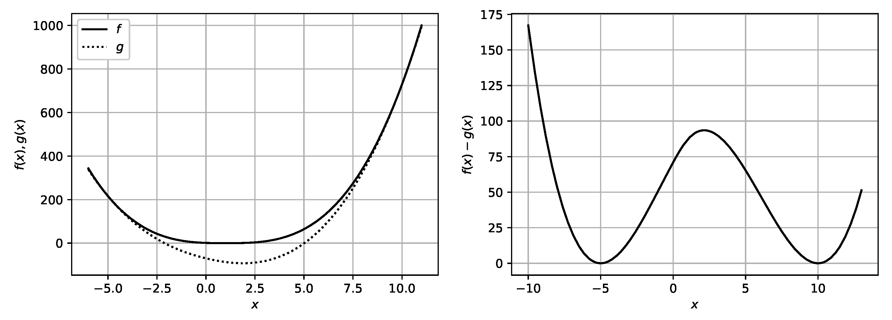
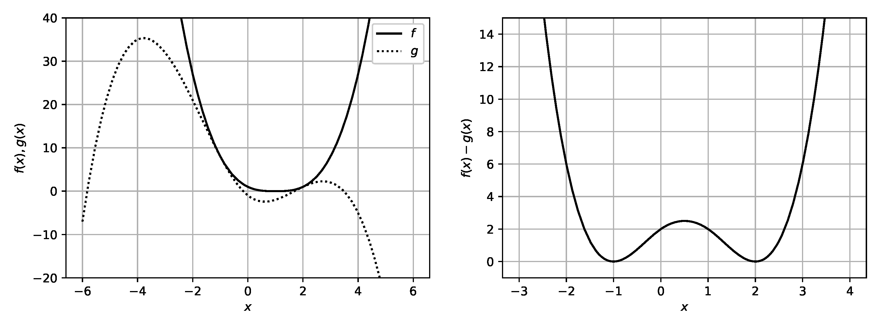
be the left-hand and right-hand sides of (20) with t = 1 , respectively. Figure 3, Figure 4 and Figure 5 illustrate that several variants of the location of tangency points of the functions f and g with respect to the stationary points of g are possible. On the left side of these figures are the plots of f ( x ) (solid line) and g ( x ) (dotted line), whereas on the right side, for clarity, is the plot of the difference f ( x ) g ( x ) .
Proof. 
By virtue of the relations (21)–(24), the problem is reduced to the case of t = 1 by the scale transformation. We let
f ( x ) = | x 1 | 3 , g ( x ) = a + b x + c x 2 + d | x | 3 , h ( x ) = f ( x ) g ( x ) , x R .
The coefficients a, b, c, and d given in the formulation of the lemma, were constructed so that points u and v were the tangency points of the functions g ( x ) and f ( x ) ; that is, these coefficients are defined as the solution to the system of the following four linear equations:
g ( u ) = f ( u ) , g ( u ) = f ( u ) , g ( v ) = f ( v ) , g ( v ) = f ( v ) , a + b u + c u 2 + d | u | 3 = ( 1 u ) 3 , b + 2 c u + 3 d u | u | = 3 ( 1 u ) 2 , a + b v + c v 2 + d v 3 = ( v 1 ) 3 , b + 2 c v + 3 d v 2 = 3 ( v 1 ) 2 .
Next, we proved that h ( x ) 0 for any x R .
1. Let 0 u < 1 . Then
a 1 ( u , v ) = 2 u v u v 2 u 2 v 2 2 u 2 v u 2 2 u v 2 + 4 u v v 2 u v 3 , b 1 ( u , v ) = 3 2 u 3 v 2 4 u 3 v + u 3 + 2 u 2 v 3 4 u 2 v 2 + 5 u 2 v 4 u v 3 + 5 u v 2 4 u v + v 3 u v 3 , c 1 ( u , v ) = 3 u 3 4 u 2 v 2 + 5 u 2 v 4 u 2 + 5 u v 2 4 u v + 2 u + v 3 4 v 2 + 2 v u v 3 , a n d d ( u , v ) = u + v 2 u 2 4 u v + 2 u + v 2 + 2 v 2 u v 3 .
(1a) Let x 1 . We have
h ( x ) = 2 u 1 2 x v 2 2 u v + u x 3 u 3 v x + v + 2 x u v 3 .
Since
2 ( u 1 ) 2 ( x v ) 2 0 , ( u v ) 3 < 0 ,
it suffices to show that
s 1 ( x ) : = 2 u v + u x 3 u 3 v x + v + 2 x 0 .
We have
s 1 ( 1 ) = 2 ( u 1 ) ( v 1 ) < 0 a n d
s 1 ( x ) = u 3 v + 2 < 0 , sin ce v > 1 u + 2 3 ,
therefore, s 1 ( x ) < 0 and h ( x ) 0 . Moreover, h ( x ) = 0 if and only if x = v .
(1b) Let 0 x < 1 . Then
h ( x ) = 2 x u 2 v 1 2 2 u v 3 u x + u + v x 3 v + 2 x u v 3 .
Since
2 ( x u ) 2 ( v 1 ) 2 0 , ( u v ) 3 < 0 ,
it suffices to show that
s 2 ( x ) : = ( v 3 u + 2 ) x + 2 u v + u 3 v 0 .
We have
s 2 ( 0 ) = 2 u v + u 3 v < 0 , sin ce v > 1 > u 3 2 u ; a n d
s 2 ( 1 ) = 2 ( u 1 ) ( v 1 ) < 0 ,
min { s 2 ( 0 ) , s 2 ( 1 ) } s 2 ( x ) max { s 2 ( 0 ) , s 2 ( 1 ) } ,
therefore, s 2 ( x ) < 0 and h ( x ) 0 . Moreover, h ( x ) = 0 if and only if x = u .
(1c) Let x < 0 . Then
h ( x ) = 3 ( 1 x ) 2 b 2 c x + 3 d x 2 ,
h ( x ) = 6 ( d 1 ) x + 2 ( 3 c ) ,
h ( 0 ) 0 ,
moreover, h ( 0 ) = 0 if and only if u = 0 (as it was proved above),
h ( 0 ) = b 3 = 6 u v 1 2 u 2 + u v 2 v v u 3 ,
d 1 = 2 u 1 2 u 3 v + 2 v u 3 ,
3 c = 6 v 1 2 2 u 2 u v u v 3 .
Taking into account the relations
6 u ( v 1 ) 2 ( v u ) 3 0 ,
u 2 + u v 2 v < 0 , sin ce v > 1 > u 2 2 u ,
we have h ( 0 ) 0 . Moreover, h ( 0 ) = 0 if and only if u = 0 . Note that
2 ( u 1 ) 2 ( v u ) 3 > 0 ,
u 3 v + 2 < 0 , sin ce v > 1 > u + 2 3 ,
6 ( v 1 ) 2 ( u v ) 3 < 0 ,
2 u 2 u v < 0 , sin ce v > 1 > 2 u 2 u ,
therefore, d 1 < 0 , 3 c > 0 , and h ( x ) > 0 . Hence, h ( x ) increases, and with the account of h ( 0 ) 0 , we find that h ( x ) < 0 for x < 0 ; that is, h ( x ) decreases for x < 0 . Since h ( 0 ) 0 , we have h ( x ) > 0 for x < 0 .
2. Now let u < 0 . We have
a 1 ( u , v ) = 6 u 4 v 2 u 4 12 u 3 v 2 + 4 u 3 v + 6 u 2 v 4 12 u 2 v 3 + 6 u 2 v 2 + 4 u v 3 v 4 u v u + v u 2 4 u v + v 2 , b 1 ( u , v ) = 3 4 u 3 v u 3 4 u 2 v 2 3 u 2 v + 4 u v 3 3 u v 2 + 4 u v v 3 u v u 2 4 u v + v 2 , c 1 ( u , v ) = 3 u 4 + 4 u 3 v 4 u 3 6 u 2 v 2 + 2 u 2 + 4 u v 3 + v 4 4 v 3 + 2 v 2 u v u + v u 2 4 u v + v 2 , d ( u , v ) = u + v 2 u 2 4 u v + 2 u + v 2 + 2 v 2 u + v u 2 4 u v + v 2 .
(2a) Let x 1 . Then
h ( x ) = 2 x v 2 s 3 ( x ) v u u + v u 2 4 u v + v 2 ,
where
s 3 ( x ) = 3 u 4 6 u 3 + 3 u 2 v 2 + 6 u 2 v x 6 u 2 v 3 u 2 x + 3 u 2 6 u v 2 x + 4 u v + 2 u x + 3 v 2 x v 2 2 v x .
Note that
2 ( x v ) 2 ( v u ) ( u + v ) ( u 2 4 u v + v 2 ) 0
with the equality attained iff x = v . Therefore, it suffices to show that s 3 ( x ) > 0 . However, this follows from the relations
s 3 ( 1 ) = 3 u 4 6 u 3 + 3 u 2 v 2 2 u ( v 1 ) ( 3 v + 1 ) + 2 v ( v 1 ) > 0 ,
s 3 ( x ) = 3 u 2 ( 2 v 1 ) 2 u ( 3 v 2 1 ) + v ( 3 v 2 ) > 0 .
(2b) Let x 0 . Then
h ( x ) = 2 ( x u ) 2 s 4 ( x ) ( v u ) ( u + v ) ( u 2 4 u v + v 2 ) ,
where
s 4 ( x ) = 3 u 2 v 2 6 u 2 v x + 3 u 2 x u 2 + 6 u v 2 x 6 u v 2 + 4 u v 2 u x + 3 v 4 6 v 3 3 v 2 x + 3 v 2 + 2 v x .
Note that
2 ( x u ) 2 ( v u ) ( u + v ) ( u 2 4 u v + v 2 ) 0 ,
with the equality attained iff x = u . Therefore, it suffices to show that s 4 ( x ) > 0 . However, this follows from the relations
s 4 ( 0 ) = u 2 ( 3 v 2 1 ) 2 u v ( 3 v 2 ) + 3 v 2 ( v 1 ) 2 > 0 ,
s 4 ( x ) = ( v u ) ( 3 u ( 2 v 1 ) ( 3 v 2 ) ) < 0 .
(2c) Let 0 < x < 1 . For all u < 0 , v > 1 , u + v > 0 , we have
h ( 0 ) = 2 u 2 u 2 ( 3 v 2 1 ) 2 u v ( 3 v 2 ) + 3 v 2 ( v 1 ) 2 v u u + v u 2 4 u v + v 2 > 0 ,
h ( 1 ) = 2 v 1 2 3 u 4 6 u 3 + 3 u 2 v 2 2 u 3 v 2 2 v 1 + 2 v ( v 1 ) v u u + v u 2 4 u v + v 2 > 0 ,
h ( 0 ) = 6 u u 2 2 v 1 u v 2 v 1 + 2 v ( v 1 ) 2 v u u 2 4 u v + v 2 > 0 .
Moreover,
h ( x ) = 12 ( 1 u v ) ( u 2 + u ( 1 4 v ) + v 2 + v 2 ) ( u + v ) ( u 2 4 u v + v 2 ) 0 u + v 1 .
Consider the case u + v 1 . Since h ( x ) 0 , the function h is concave. Since h ( 0 ) > 0 , the function h has at most one root x 0 on the interval 0 x 1 . Moreover, h ( x ) 0 for 0 x x 0 and h ( x ) 0 for x 0 x 1 . Therefore, h ( x ) either increases on the whole interval 0 x 1 (if h is nonnegative), or increases on 0 x x 0 and decreases on x 0 x 1 , so that
min 0 x 1 h ( x ) = min { h ( 0 ) , h ( 1 ) } .
Since h ( 0 ) > 0 and h ( 1 ) > 0 , we have h ( x ) > 0 .
Now consider the case 0 < u + v < 1 . In this case, h is convex. Note that
h ( 1 ) = 6 v 1 2 u v 2 u 3 2 u 2 v + u 2 v 2 v 1 v ( v 1 ) v u u + v u 2 4 u v + v 2 < 0 .
Since h ( 0 ) > 0 , h ( 1 ) < 0 , and h is convex, the function h has exactly one root x 1 on the interval 0 x 1 . Moreover, h ( x ) 0 for 0 x x 1 and h ( x ) 0 for x 1 x 1 . So, the function h increases on the interval [ 0 , x 1 ] and decreases on [ x 1 , 1 ] . Therefore,
min 0 x 1 h ( x ) = min { h ( 0 ) , h ( 1 ) } .
With the account of h ( 0 ) > 0 and h ( 1 ) > 0 , we have h ( x ) > 0 for all 0 x 1 .     □
Lemma 1 trivially yields the following statement.
Lemma 2.
For any L ( X ) P , t R { 0 } and every u , v R such that
u + v > 0 , u < 1 < v ,
the inequality
E | X t | 3 a t ( u , v ) + b t ( u , v ) E X + c t ( u , v ) E X 2 + d ( u , v ) E | X | 3 ,
holds with equality attained iff the distribution of the r.v. X is concentrated in the two points: u t and v t .
By P 2 , let us denote the class of all the non-degenerate two-point distributions. Obviously, P 2 P .
Lemma 3.
For any t ( 0 , 1 )
H ( t ) : = sup L ( X ) P : E X = t , E X 2 = 1 E | X | 3 E | X t | 3 = sup L ( X ) P 2 : E X = t , E X 2 = 1 E | X | 3 E | X t | 3 ,
moreover, the least upper bound on the right-hand side can be attained only on the two-point distributions.
Proof. 
It suffices to prove that for any ϱ 1 and r.v. X with
E X = t , E X 2 = 1 , a n d E | X | 3 = ϱ
there exists a two-point r.v. Y with
E Y = t , E Y 2 = 1 , a n d E | Y | 3 = ϱ ,
satisfying the inequality
E | X t | 3 E | Y t | 3 .
Indeed, the above moment conditions imply that
H ( t ) = sup ϱ 1 sup L ( X ) P : E X = t , E X 2 = 1 , E | X | 3 = ϱ ϱ E | X t | 3 sup ϱ 1 sup Y P 2 : E Y = t , E Y 2 = 1 , E | Y | 3 = ϱ ϱ E | Y t | 3 , 0 < t < 1 ,
where only equality is possible since P 2 P .
(1) Let ϱ > 1 . Consider a two-point r.v. Y p that takes values x > y with probabilities p and q = 1 p , respectively, and satisfies E Y p = t , E Y p 2 = 1 . Then we necessarily have
x = x ( p ) = t + ( 1 t 2 ) q / p , y = y ( p ) = t ( 1 t 2 ) p / q .
We show that x + y > 0 iff p < 1 + t 2 . We have
x + y > 0 2 t p q + 1 t 2 ( q p ) p q > 0 2 t p ( 1 p ) > 1 t 2 ( 2 p 1 ) .
The last inequality trivially holds for 0 < p 1 2 since the left-hand side is positive, whereas the right-hand side is non-positive. If 1 2 < p < 1 , then both sides of this inequality are positive. Therefore, they can be squared:
4 t 2 p ( 1 p ) > ( 1 t 2 ) ( 4 p 2 4 p + 1 ) t 2 > ( 2 p 1 ) 2 p < 1 + t 2 .
Unifying the intervals under consideration, we obtain the desired statement. Note that on 0 , 1 + t 2 the function
ϱ ˜ ( p ) E | Y p | 3 = p t + q p ( 1 t 2 ) 3 + q | t p q ( 1 t 2 ) | 3
of the argument, p takes all the values from the interval ( 1 , + ) because, for any 0 < t < 1 , we have
ϱ ˜ 1 + t 2 = 1 , lim p 0 + ϱ ˜ ( p ) = +
and ϱ ˜ ( p ) is continuous. Hence, for every ϱ > 1 there exists p 0 = p 0 ( ϱ ) 0 , 1 + t 2 such that E | Y p 0 | 3 = ϱ . Furthermore, note that,
y ( p 0 ) < t < x ( p 0 ) , x ( p 0 ) + y ( p 0 ) > 0 ,
and, hence, the couple u = y ( p 0 ) / t a n d v = x ( p 0 ) / t satisfy all the conditions of Lemma 2, according to which, with the account of the definition of the r.v. Y p 0 , we have
E | X t | 3 a t ( u , v ) + b t ( u , v ) t + c t ( u , v ) + d ( u , v ) ϱ = E | Y p 0 t | 3 ,
where the equality is attained iff the distribution of the r.v. X is concentrated in exactly two points u t = y ( p 0 ) and v t = x ( p 0 ) ; that is, iff X = d Y p 0 . Therefore, the desired statement holds with the r.v. Y = d Y p 0 .
(2) Now let ϱ = 1 . By virtue of Jensen’s inequality, for the strictly convex function f ( x ) = x 3 / 2 , x 0 , we have
1 = E | X | 3 = E f ( X 2 ) f ( E X 2 ) = f ( 1 ) = 1 ,
where the equality holds iff
P ( X 2 = E X 2 ) = 1 , i . e . , P ( | X | = 1 ) = 1 .
The condition E X = t immediately implies that, in this case, the r.v. X must have the two-point distribution of the form P ( X = ± 1 ) = ( 1 ± t ) / 2 . So, the desired statement holds with Y = d X . □

4. Analysis of Two-Point Distributions

Recall that by P 2 , we denoted the class of all the non-degenerate two-point distributions.
Lemma 4.
(a)For any t ( 0 , 1 )
sup L ( X ) P 2 : E X = t , E X 2 = 1 E | X | 3 E | X t | 3 = max 1 < z < 1 M ( z , t ) = M ( z ( t ) , t ) ,
where the function z ( t ) , t ( 0 , 1 ) , is defined in Theorem 1 (see (9))
M ( z , t ) = M 1 ( z , t ) , 1 < z < 1 2 t 2 , M 2 ( z , t ) , 1 2 t 2 z < 1 ,
M 1 ( u , t ) = 1 + 3 t 2 1 t 2 · 1 u 2 a ( t ) u 1 u 2 1 + u 2 , u ( 1 , 1 ) ,
M 2 ( v , t ) = b ( t ) 1 v 2 + 2 v v 2 + 1 , v ( 1 , 1 ) ,
a ( t ) = 4 t 2 3 3 t 1 t 2 , b ( t ) = t ( 3 2 t 2 ) ( 1 t 2 ) 3 / 2 , t ( 0 , 1 ) .
Moreover, the supremum in (25) is attained only on the two-point distribution defined in Theorem 1 (see (12)).
(b)The functions M , M 1 , a n d M 2 are differentiable in the domain ( z , t ) ( 1 , 1 ) × ( 0 , 1 ) and have continuous derivatives there.
(c)There hold the equalities
lim z 1 + M 1 ( z , t ) = lim z 1 M 1 ( z , t ) = 1 , t ( 0 , 1 ) ,
lim z 1 + M 2 ( z , t ) = 1 , lim z 1 M 2 ( z , t ) = 1 , t ( 0 , 1 ) ,
lim t 0 M 1 ( z , t ) = 1 , lim t 0 M 2 ( z , t ) = 2 z z 2 + 1 , z ( 1 , 1 ) ,
lim t 1 M 2 ( z , t ) = + , z ( 1 , 1 ) .
(d)The function z ( t ) is continuously differentiable and monotonically decreasing on the interval t ( 0 , 1 ) with
z ( 0 + ) = 3 3 , z ( t 0 ) = 7 2 3 , z ( 1 ) = 0 .
Moreover, the inequalities
z ( t ) 1 2 t 2 , t ( 0 , t 0 ] ,
z ( t ) 1 2 t 2 , t [ t 0 , 1 ) ,
hold, and the equality in each of them is attained only at the endpoint t = t 0 : = 5 7 6 = 0.6263 , defined in Theorem 1.
Proof. 
(a) Consider a two-point distribution
P ( X = x ) = p = 1 P ( X = y ) = 1 q ,
with some x > t > y , p ( 0 , 1 ) . From the conditions
E X = t a n d E X 2 = 1 ,
it follows that
x = t + q p ( 1 t 2 ) a n d y = t p q ( 1 t 2 ) .
Denote
H ˜ ( p , t ) = E | X | 3 E | X t | 3 = p | x | 3 + q | y | 3 p ( x t ) 3 + q ( t y ) 3 , p ( 0 , 1 ) , t ( 0 , 1 ) .
Then
H ˜ ( t ) : = sup L ( X ) P 2 : E X = t , E X 2 = 1 E | X | 3 E | X t | 3 = sup 0 < p < 1 H ˜ ( p , t ) .
Let us show that the last supremum has the form (25) with z ( t ) defined in (9).
For 0 < p t 2 , we have y 0 and
H ˜ ( p , t ) = p x 3 + q y 3 p ( x t ) 3 + q ( t y ) 3 = t ( 3 2 t 2 ) + q p p q ( 1 t 2 ) 3 / 2 p 2 + q 2 p q ( 1 t 2 ) 3 / 2 = b ( t ) p q + ( q p ) p 2 + q 2 .
For t 2 < p < 1 , we have y < 0 and
H ˜ ( p , t ) = 1 + t ( 4 t 2 3 ) ( p q ) + 6 t 2 1 t 2 p q p 2 + q 2 p q ( 1 t 2 ) 3 / 2 = 1 + 3 t 2 1 t 2 · a ( t ) p q ( p q ) + 2 p q p 2 + q 2 .
In terms of a new variable
z = q p = 1 2 p ,
we have
p q = 1 z 2 4 , p 2 + q 2 = 1 + z 2 2 , and sup p ( 0 , 1 ) H ˜ ( p , t ) = sup z ( 1 , 1 ) H ˜ 1 z 2 , t
Observing that
H ˜ 1 z 2 , t = M ( z , t ) ,
we may finally write
H ˜ ( t ) : = sup p ( 0 , 1 ) H ˜ ( p , t ) = sup 1 < z < 1 M ( z , t ) , t ( 0 , 1 ) .
We show that z ( t ) is the unique global maximum point of the function M ( · , t ) for each t ( 0 , 1 ) , whence, with the account of relations (26), (27), (30), the item (a) would follow.
For M 1 , we have
M 1 ( u , t ) u = 3 t 2 1 t 2 · a ( t ) ( 3 u 2 1 ) 4 u 1 u 2 1 u 2 · ( 1 + u 2 ) 2 ,
and hence, the stationary points of M 1 ( · , t ) can be determined from the equation
g ( u ) : = 4 u 1 u 2 3 u 2 1 = a ( t ) ,
which coincides with (10).
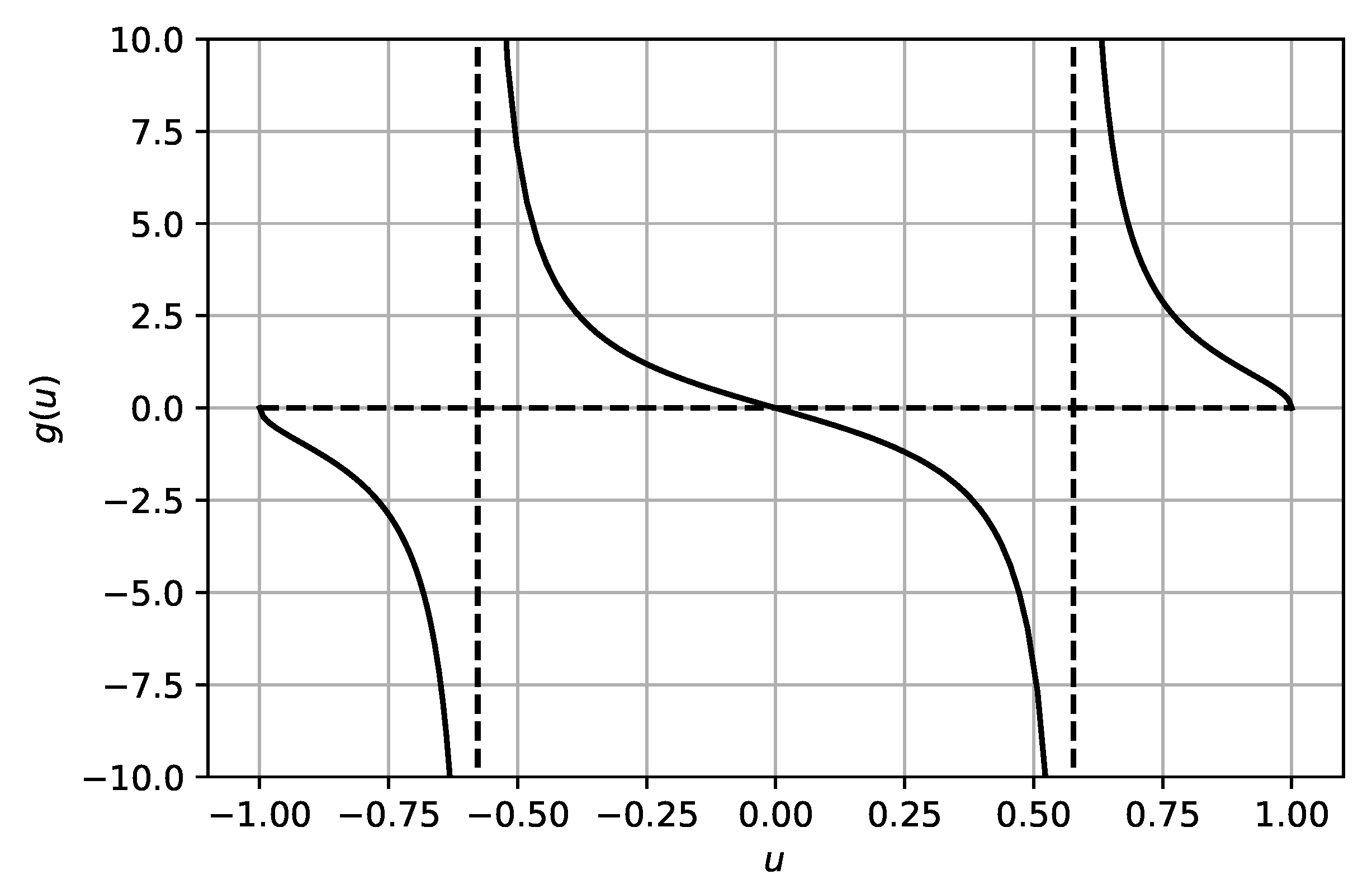
Note that the function g ( u ) is even, continuously differentiable and monotonically decreasing on the intervals ( 1 , 3 / 3 ) , ( 3 / 3 , 3 / 3 ) , and ( 3 / 3 , 1 ) and has discontinuity points of the second kind in the points u = ± 3 / 3 (see the plot of g ( u ) in Figure 6). Therefore, there exist the inverse functions
g 1 1 : ( , 0 ) ( 1 , 3 / 3 ) ,
g 2 1 : R ( 3 / 3 , 3 / 3 ) ,
g 3 1 : ( 0 , + ) ( 3 / 3 , 1 ) ,
each of which is differentiable and monotonically decreasing in its domain.
If a ( t ) = 0 (that is, t = 3 / 2 ), then it is easy to make sure that u = 0 is the unique maximum point and unique stationary point of the function M 1 ( · , t ) on ( 1 , 1 ) .
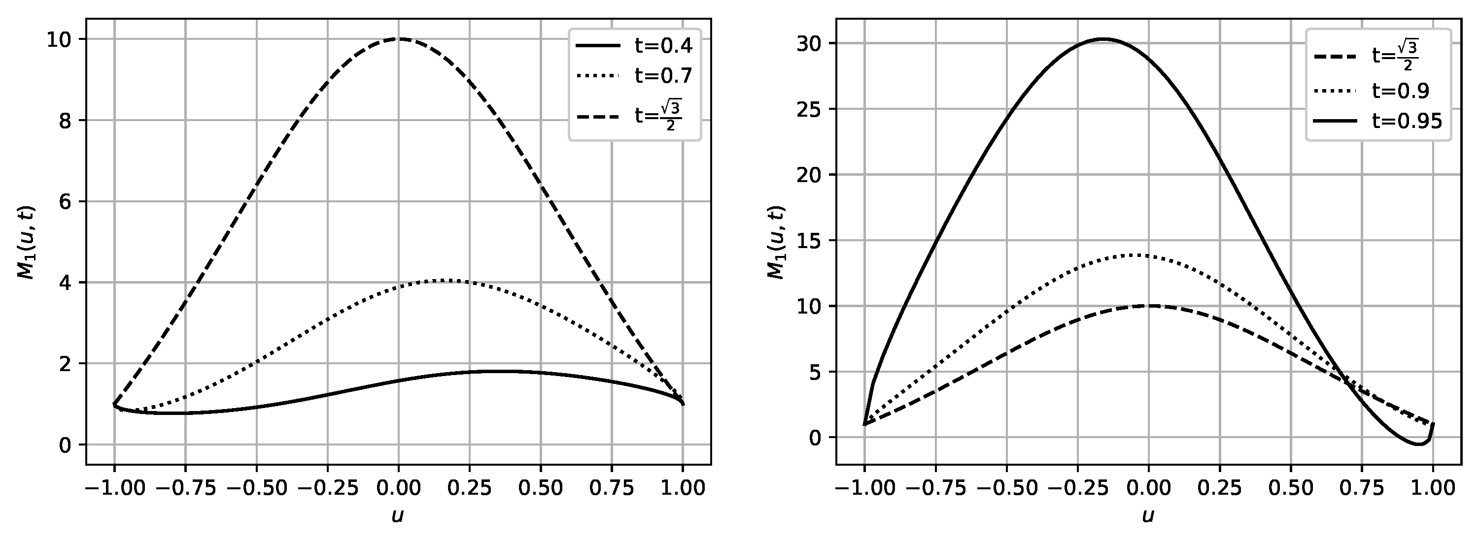
Now let a ( t ) 0 . By u 1 ( t ) < u 2 ( t ) denote the roots of the equation g ( u ) = a ( t ) on the interval u ( 1 , 1 ) . If a ( t ) > 0 (that is, t > 3 / 2 ), then u 1 ( t ) = g 2 1 ( a ( t ) ) , u 2 ( t ) = g 3 1 ( a ( t ) ) are respectively the points of local maximum and minimum of the function M 1 ( · , t ) (see the plots of the function M 1 ( · , t ) for some t in Figure 7). Moreover, a ( t ) u 1 ( t ) < 0 and M 1 ( u 1 ( t ) , t ) > 1 . Since a ( t ) is continuously differentiable and monotonically increasing, both u 1 ( · ) and u 2 ( · ) are continuously differentiable and monotonically decreasing with
u 1 ( 3 / 2 + ) = 0 , u 1 ( 1 ) = 3 / 3 ,
u 2 ( 3 / 2 + ) = 1 , u 2 ( 1 ) = 3 / 3 .
And if a ( t ) < 0 (that is, t < 3 / 2 ), then u 1 ( t ) = g 1 1 ( a ( t ) ) , u 2 ( t ) = g 2 1 ( a ( t ) ) are the points of local minimum and maximum, respectively. Moreover, a ( t ) u 2 ( t ) < 0 and M 1 ( u 2 ( t ) , t ) > 1 . Since a ( t ) is continuously differentiable and monotonically increasing, both u 1 ( t ) and u 2 ( t ) are continuously differentiable and monotonically decreasing on the interval t ( 0 , 3 / 2 ) with
u 1 ( 0 + ) = 3 / 3 , u 1 ( 3 / 2 ) = 1 ,
u 2 ( 0 + ) = 3 / 3 , u 2 ( 3 / 2 ) = 0 .
Since M 1 ( ± 1 , t ) = 1 , the local maximum point of the function M 1 ( · , t ) is the point of its global maximum on the whole interval u ( 1 , 1 ) .
So, for an arbitrary s ( 1 , 1 ) , we have
sup 1 < u < s M 1 ( u , t ) = M 1 ( 0 s , t ) , a ( t ) = 0 , M 1 ( u 1 ( t ) s , t ) , a ( t ) > 0 , M 1 ( u 2 ( t ) s , t ) 1 , a ( t ) < 0
(here, the symbols ∨ and ∧ denote the maximum and minimum, respectively). For s = 1 2 t 2 , we have
sup 1 < u < 1 2 t 2 M 1 ( u , t ) = M 1 1 2 , 3 2 = 32 5 , t = 3 / 2 , M 1 ( u 1 ( t ) ( 1 2 t 2 ) , t ) , 3 / 2 < t < 1 , M 1 ( u 2 ( t ) ( 1 2 t 2 ) , t ) 1 , 0 < t < 3 / 2 .
Compare 1 2 t 2 with u 2 ( t ) for 0 < t < 3 2 and with u 1 ( t ) for 3 2 < t < 1 . If 3 2 < t < 1 , then, as it has already been noted, 3 / 3 < u 1 ( t ) < 0 , and hence, u 1 ( t ) > 3 / 3 1 2 t 2 trivially for 1 2 + 3 6 t < 1 . And if t 3 2 , 1 2 + 3 6 = ( 0.866 , 0.888 ) , then 1 2 t 2 3 3 , 1 2 3 3 , 3 3 , that is, point 1 2 t 2 belongs to the same interval 3 3 , 3 3 of the monotonic decrease of the function g ( u ) , as u 1 ( t ) , and hence, on the interval of the values of t under consideration, we have
1 2 t 2 u 1 ( t ) g ( 1 2 t 2 ) g ( u 1 ( t ) ) a ( t )
4 t ( 2 t 2 1 ) 1 t 2 6 t 4 + 6 t 2 1 4 t 2 3 3 t 1 t 2
12 t 2 ( 2 t 2 1 ) ( 1 t 2 ) ( 4 t 2 3 ) ( 6 t 4 + 6 t 2 1 ) 6 t 4 10 t 2 + 3 0
t 5 7 6 , 5 + 7 6 3 2 , 1 2 + 3 6 = 3 2 , 1 2 + 3 6 .
(In the third step here, we also took into account that 6 t 4 + 6 t 2 1 > 0 for t 1 2 3 6 , 1 2 + 3 6 3 2 , 1 2 + 3 6 ) . So, unifying the obtained interval with the domain t 1 2 + 3 6 , we finally conclude that
u 1 ( t ) > 1 2 t 2 for all t 3 2 , 1 .
It remains to compare 1 2 t 2 with u 2 ( t ) on the interval 0 < t < 3 2 . As it has already been noted, on this interval, we have 0 < u 2 ( t ) < 3 3 , and hence, u 2 ( t ) > 0 1 2 t 2 a fortiori for 0.707 = 2 2 t < 3 2 and u 2 ( t ) < 3 / 3 1 2 t 2 for 0 < t 1 2 3 6 = 0.459 If t 1 2 3 6 , 2 2 , then 1 2 t 2 0 , 3 3 3 3 , 3 3 ; that is, the point 1 2 t 2 belongs to the same interval 3 3 , 3 3 of the monotonic decrease of the function g ( u ) , as u 2 ( t ) , and hence,
1 2 t 2 u 2 ( t ) g ( 1 2 t 2 ) g ( u 2 ( t ) ) a ( t ) .
Further calculations completely coincide with what has been done for the comparison of u 1 ( t ) and 1 2 t 2 , including the remark on the positiveness of the polynomial 6 t 4 + 6 t 2 1 on the interval t 1 2 3 6 , 2 2 . Therefore, for t under consideration, we have
u 2 ( t ) 1 2 t 2 t 5 7 6 , 5 + 7 6 1 2 3 6 , 2 2 = 5 7 6 , 2 2 ,
u 2 ( t ) < 1 2 t 2 t 1 2 3 6 , 5 7 6 .
Unifying the obtained domains of the values of t, we finally get
u 2 ( t ) 1 2 t 2 on the interval t 0 , 3 2 5 7 6 = : t 0 t < 3 2 ,
with equality attained only at the point t = t 0 .
Taking into account that u 2 ( t ) is the global maximum point of the function M 1 ( · , t ) for 0 < t < 3 / 2 , and also that
M 1 ( 1 2 t 2 , t ) | t = 3 / 2 = M 1 1 2 , 3 2 ,
we conclude that
max 1 < u < 1 2 t 2 M 1 ( u , t ) = M 1 ( u 2 ( t ) , t ) , 0 < t < t 0 , M 1 ( 1 2 t 2 , t ) 1 , t 0 t < 3 2 , M 1 ( 1 2 t 2 , t ) , 3 2 t < 1 .
We now consider the behavior of the function M 2 ( · , t ) . Since both functions 1 v 2 / ( v 2 + 1 ) and v / ( v 2 + 1 ) increase for v ( 1 , 0 ] , M 2 ( v , t ) increases in v ( 1 , 0 ] for every t ( 0 , 1 ) .
The numerator of the derivative
M 2 ( v , t ) v = b ( t ) v ( v 2 3 ) + 2 ( 1 v 2 ) 3 / 2 1 v 2 · ( v 2 + 1 ) 2
decreases on the interval v ( 0 , 1 ) and takes the values 2 > 0 and 2 b ( t ) < 0 of different signs at the endpoints. Therefore, the equation M 2 v = 0 , which is equivalent to
f ( v ) : = 2 ( 1 v 2 ) 3 / 2 v ( 3 v 2 ) = b ( t )
and coincides with (11), has a unique root on ( 0 , 1 ) , which is the maximum point of M 2 ( v , t ) on the interval v [ 0 , 1 ] . Since the function f ( v ) is continuously differentiable and monotonically decreasing on the interval v ( 0 , 1 ) with f ( + 0 ) = + , f ( 1 ) = 0 , there exists an inverse function
f 1 : ( 0 , + ) ( 0 , 1 ) ,
which is also continuously differentiable and monotonically decreasing. Furthermore, since the function b ( t ) is continuously differentiable and monotonically increasing on the interval t ( 0 , 1 ) , Equation (33) has a unique root
v ( t ) = f 1 ( b ( t ) ) ,
on v ( 0 , 1 ) , which is the global maximum point of the function M 2 ( · , t ) on the whole interval ( 1 , 1 ) (see the plots of the function M 2 ( · , t ) for some t in Figure 8). Moreover, v ( t ) is continuously differentiable and monotonically decreasing for t ( 0 , 1 ) , as a superposition of two continuously differentiable functions, one of which ( b ( t ) ) increases, whereas the other one ( f 1 ( b ) ) decreases. By conducting direct calculations we make sure that b ( 0 ) = 0 , b ( 1 ) = + , and hence, v ( 0 + ) = 1 , v ( 1 ) = 0 .
So, for an arbitrary s ( 1 , 1 ) , we have
sup s v < 1 M 2 ( v , t ) = M 2 ( v ( t ) s , t ) .
In particular, for s = 1 2 t 2 we obtain
sup 1 2 t 2 v < 1 M 2 ( v , t ) = M 2 ( v ( t ) ( 1 2 t 2 ) , t ) .
Compare v ( t ) and 1 2 t 2 . Since v ( t ) ( 0 , 1 ) for all t ( 0 , 1 ) by definition, a fortiori v ( t ) > 0 1 2 t 2 for 2 2 t < 1 . On the interval 0 < t < 2 2 , we have
1 2 t 2 v ( t ) f ( 1 2 t 2 ) f ( v ( t ) ) b ( t )
8 t 3 ( 1 t 2 ) 3 / 2 ( 2 t 2 1 ) ( 2 t 4 2 t 2 1 ) t ( 3 2 t 2 ) ( 1 t 2 ) 3 / 2
8 t 2 ( 1 t 2 ) 3 ( 3 2 t 2 ) ( 2 t 2 1 ) ( 2 t 4 2 t 2 1 ) 6 t 4 10 t 2 + 3 0
t 5 7 6 , 5 + 7 6 0 , 2 2 = 5 7 6 , 2 2 = [ 0.626 , 0.707 ) .
On the third step here we also took into account the fact that 2 t 2 1 < 0 , 2 t 4 2 t 2 1 < 0 in the domain of the values of t under consideration. Thus, unifying the obtained interval with the domain t 2 / 2 , we arrive at
v ( t ) 1 2 t 2 on the interval t ( 0 , 1 ) t 0 t < 1 ,
with equality attained only at the point t = t 0 .
So, for s = 1 2 t 2 we finally obtain
max 1 2 t 2 v < 1 M 2 ( v , t ) = M 2 ( 1 2 t 2 , t ) , 0 < t < t 0 , M 2 ( v ( t ) , t ) , t 0 t < 1 .
As a by-product we showed that
u 2 ( t 0 ) = v ( t 0 ) = 1 2 t 0 2 = 7 2 3 = 0.21525 .
In addition, note that the function
M 1 ( 1 2 t 2 , t ) = 1 ( 1 t 2 ) ( 2 t 4 2 t 2 + 1 ) = M 2 ( 1 2 t 2 , t ) , t ( 0 , 1 ) ,
increases monotonically on the interval t 0 t 3 2 .
Finally, from (29), (31), (32), (34), (36), it follows that
H ˜ ( t ) = sup 1 < z < 1 H ˜ 1 z 2 , t = max max 1 < u < 1 2 t 2 M 1 ( u , t ) , max 1 2 t 2 v < 1 M 2 ( v , t ) =
= M 1 ( u 2 ( t ) , t ) M 2 ( 1 2 t 2 , t ) , 0 < t < t 0 , M 1 ( 1 2 t 2 , t ) M 2 ( v ( t ) , t ) 1 , t 0 t < 3 2 , M 1 ( 1 2 t 2 , t ) M 2 ( v ( t ) , t ) , 3 2 t < 1 , =
= M 1 ( u 2 ( t ) , t ) M 1 ( 1 2 t 2 , t ) , 0 < t < t 0 , M 2 ( 1 2 t 2 , t ) M 2 ( v ( t ) , t ) 1 , t 0 t < 3 2 , M 2 ( 1 2 t 2 , t ) M 2 ( v ( t ) , t ) , 3 2 t < 1 .
Taking into account that
M 1 ( 1 2 t 0 2 , t 0 ) = M 2 ( 1 2 t 0 2 , t 0 ) = 54 8 7 4 = 3.14575 > 1 ,
we obtain
H ˜ ( t ) = M 1 ( u 2 ( t ) , t ) M 1 ( 1 2 t 2 , t ) , 0 < t < t 0 , M 2 ( 1 2 t 2 , t ) M 2 ( v ( t ) , t ) , t 0 t < 1 .
Recalling that v ( t ) is the unique point of global maximum of M 2 ( v , t ) on the interval v ( 1 , 1 ) , and u 2 ( t ) is the unique point of global maximum of M 1 ( u , t ) on the interval u ( 1 , 1 ) for t ( 0 , t 0 ] 0 , 3 2 (when a ( t ) < 0 ), we conclude that
H ˜ ( t ) = M 1 ( u 2 ( t ) , t ) , 0 < t < t 0 , M 2 ( v ( t ) , t ) , t 0 t < 1 , = M ( z ( t ) , t ) .
Thus, the function u 2 ( t ) defined for t ( 0 , 3 / 2 ) (which corresponds to the case a ( t ) < 0 ) and monotonically decreasing in its domain, acts as the function u ( t ) given in the formulation of Theorem 1 and the lemma being proved, whereas the role of the global maximum point z ( t ) of the function M ( · , t ) is played by the functions u ( t ) = u 2 ( t ) for t ( 0 , t 0 ) and v ( t ) for t [ t 0 , 1 ) , which completely agrees with (9).
(b) The functions M 1 and M 2 are obviously differentiable in the domain ( z , t ) ( 1 , 1 ) × ( 0 , 1 ) and have continuous partial derivatives there. It is easy to see from (27) and (28) that the function H ˜ ( p , t ) is differentiable in the domain ( p , t ) ( 0 , 1 ) × ( 0 , 1 ) and has continuous partial derivatives there. With the account of (31) we conclude that M is differentiable in the domain ( z , t ) ( 1 , 1 ) × ( 0 , 1 ) and has continuous partial derivatives there.
(c) This statement can be verified directly.
(d) We show that z ( t ) is continuously differentiable and decreases on the interval t ( 0 , 1 ) . Since u 2 ( t ) is continuously differentiable and monotonically decreasing on the interval t 0 , 3 2 0 , t 0 and the function v ( t ) is continuously differentiable and monotonically decreasing on the interval t ( 0 , 1 ) t 0 , 1 , with the account of (35), we conclude that the function z ( t ) is continuous and monotonically decreasing on the interval t ( 0 , 1 ) . Furthermore, the function z ( t ) is continuously differentiable on each of the intervals 0 , t 0 and t 0 , 1 . In addition, we show that u 2 ( t 0 ) = v ( t 0 ) , whence it will follow that the function z is continuously differentiable in the point t 0 , and hence, on the whole, interval t ( 0 , 1 ) . In the neighborhood of t 0 , we have
u 2 ( t 0 ) = g 1 ( a ( t 0 ) ) , v ( t 0 ) = f 1 ( b ( t 0 ) ) ,
therefore,
u 2 ( t 0 ) = a ( t 0 ) g ( u 2 ( t 0 ) ) , v ( t 0 ) = b ( t 0 ) f ( v ( t 0 ) ) ,
whence by virtue of (35), we obtain
u 2 ( t 0 ) = a ( t 0 ) g ( 1 2 t 0 2 ) , v ( t 0 ) = b ( t 0 ) f ( 1 2 t 0 2 ) .
By direct calculations, we make sure that
u 2 ( t 0 ) = v ( t 0 ) = 2 3 7 3 = 0.687263 .
Thus, the function z ( t ) is differentiable on the interval t ( 0 , 1 ) .
Now to complete the proof of item (d), it remains to recall that
z ( 0 + ) = u 2 ( 0 + ) = 3 3 , z ( 1 ) = v ( 1 ) = 0 , z ( t 0 ) = u 2 ( t 0 ) = v ( t 0 ) = 7 2 3 ,
and that (see the proof of item (a)) each of the equations
u 2 ( t ) = 1 2 t 2 , t 0 , 3 / 2 ,
v ( t ) = 1 2 t 2 , t ( 0 , 1 ) ,
has the unique root t = t 0 . □

5. Proofs of Main Results

Proof of Theorem 1 
It is obvious that H ( 0 ) = 1 and H is an even function. Since J ( X ) is invariant with respect to the scale transform of X, the single non-linear condition in (8) can be replaced by the two linear ones: E X = t , E X 2 = 1 . Further, from Lemmas 3 and 4 (a), (d), it follows that for t ( 0 , 1 ) , we have
H ( t ) = M ( z ( t ) , t ) = M 1 ( z ( t ) , t ) , 1 < z ( t ) < 1 2 t 2 , M 2 ( z ( t ) , t ) , 1 2 t 2 z ( t ) < 1 , =
= 1 + 3 t 2 1 t 2 · 1 z 2 ( t ) a ( t ) z ( t ) 1 z 2 ( t ) 1 + z 2 ( t ) , 0 < t < t 0 , b ( t ) 1 z 2 ( t ) + 2 z ( t ) z 2 ( t ) + 1 , t 0 t < 1 .
By the definition of the function z ( t ) , we have
a ( t ) = 4 z ( t ) 1 z 2 ( t ) 3 z 2 ( t ) 1 , 0 < t < t 0 ,
b ( t ) = 2 ( 1 z 2 ( t ) ) 3 / 2 z ( t ) ( 3 z 2 ( t ) ) , t 0 t < 1 .
Hence,
H ( t ) = 1 + 3 t 2 1 t 2 · 1 z 2 ( t ) 1 3 z 2 ( t ) , 0 < t < t 0 , 2 z ( t ) ( 3 z 2 ( t ) ) , t 0 t < 1 ,
which coincides with (8). The form and uniqueness of the extreme distribution were proved in Lemma 4 ( a ).
It remains to be proven that the function H is continuous and monotonically increasing on the interval t [ 0 , 1 ) and that H ( 1 ) = + . By virtue of Lemma 4 ( a ) for t ( 0 , 1 ) , we have H ( t ) = M ( z ( t ) , t ) , moreover, M is continuous in the domain ( z , t ) ( 1 , 1 ) × ( 0 , 1 ) , whereas z is continuous on the interval t ( 0 , 1 ) , whence H ( t ) is continuous on the interval t ( 0 , 1 ) . Since
H ( 0 + ) = M ( z ( 0 + ) , 0 + ) = 1 = H ( 0 ) ,
H is also continuous in zero.
Finally, prove that the function H is monotonically increasing. From the definition of the function z ( t ) , it follows that
1 1 3 z 2 ( t ) = 3 4 t 2 12 t z ( t ) ( 1 t 2 ) ( 1 z 2 ( t ) ) , t ( 0 , t 0 ) ,
and hence, we can write
H ( t ) = 1 + t ( 3 4 t 2 ) 1 z 2 ( t ) 4 z ( t ) ( 1 t 2 ) 3 / 2 , 0 < t < t 0 , 2 z ( t ) ( 3 z 2 ( t ) ) , t 0 t < 1 .
Note that the function t ( 3 4 t 2 ) ( 1 t 2 ) 3 / 2 is positive and monotonically increasing on the interval 0 < t < t 0 , whereas the function z 1 1 z 2 is positive and monotonically decreasing on the interval 0 < z < 1 . Since the function z ( t ) decreases on the interval 0 < t < t 0 as well, we conclude that H increases on the interval ( 0 , t 0 ) as a product of two positive monotonically increasing functions (up to an additive constant). Furthermore, since the function 2 / z ( 3 z 2 ) decreases on the interval 0 < z < 1 and the function z ( t ) decreases on the interval t 0 t < 1 , the function H ( t ) increases on the interval t 0 t < 1 , as a superposition of two decreasing functions. Finally, the existence of an infinite limit of H ( t ) , as t 1 , follows from that z ( t ) 0 + , as t 1 . □
Proof of Proposition 1. 
By virtue of the continuity of H and H ^ , it suffices to prove inequality (15) only on the interval ( 0 , t 0 ) . By the definition of z ( t ) for 0 < t < t 0 , as a unique root of the equation
g ( z ) : = 4 z 1 z 2 3 z 2 1 = 4 t 2 3 3 t 1 t 2 = : a ( t ) ,
on the interval 0 < z < 3 / 3 , we have
lim t 0 + z ( t ) = 3 3 , lim t 0 + z ( t ) = lim t 0 + a ( t ) g ( z ( t ) ) = 2 6 9 ,
hence, by the Lagrange theorem,
z ( t ) = z ˜ ( t ) + o ( t ) , z ˜ ( t ) : = 3 3 2 6 9 t .
We show that z ( t ) < z ˜ ( t ) for 0 < t < t 0 . By virtue of the monotonic decrease of g ( u ) for 0 < u < 3 / 3 , we have
z ( t ) < z ˜ ( t ) g ( z ( t ) ) > g ( z ˜ ( t ) )
3 4 t 2 3 t 1 t 2 > 3 2 4 t 4 t 2 + 6 2 t + 9 3 t 3 2 2 t
( 3 4 t 2 ) ( 3 2 2 t ) < ( 3 2 4 t ) ( 4 t 2 + 6 2 + 9 ) ( 1 t 2 )
96 2 t 5 + t 4 328 96 2 + t 3 24 2 + 288 + t 2 306 12 2 +
+ t 288 108 2 + 108 2 = : s ( t ) > 0 .
We show that s ( t ) > 0 for 0 < t < t 0 . We have
s ( t ) = 480 2 t 4 + t 3 1312 384 2 + t 2 72 2 + 864 + t 612 24 2 288 108 2 ,
s ( t ) = 1920 2 t 3 + t 2 3936 1152 2 + t 144 2 + 1728 24 2 + 612 ,
s ( 3 ) ( t ) = 5760 2 t 2 + t 7872 2304 2 + 144 2 + 1728 ,
s ( 4 ) ( t ) = 11520 2 t 7872 2304 2 < 0 , t ( 0 , t 0 ) ,
therefore, s ( 3 ) ( t ) decreases for t ( 0 , t 0 ) . Since
s ( 3 ) ( 0 + ) = 144 2 + 1728 > 0 , s ( 3 ) ( t 0 ) = 1844.1499 < 0 ,
s ( t ) has a unique stationary point on the interval t ( 0 , t 0 ) , namely, the local maximum point. Taking into account that
s ( 0 + ) = 612 24 2 > 0 , s ( t 0 ) = 271.7769 > 0 ,
we conclude that s ( t ) > 0 for t ( 0 , t 0 ) , and whence, s ( t ) increases for t ( 0 , t 0 ] . Since s ( t 0 ) = 51.1066 < 0 , , we have s ( t ) < 0 for all t ( 0 , t 0 ] and hence, s ( t ) decreases for t ( 0 , t 0 ] . Finally, s ( t 0 ) = 10.8876 , therefore, s ( t ) > 0 for t ( 0 , t 0 ] . So, the inequality z ( t ) < z ˜ ( t ) is proved for t ( 0 , t 0 ) .
Note that
H ( t ) = M ( z ( t ) , t ) = 1 + 3 t 2 1 t 2 · 1 z 2 ( t ) 1 3 z 2 ( t )
for 0 < t < t 0 , moreover, the function M ( · , t ) increases on the interval 0 < z < 3 / 3 , therefore, taking into account that 0 < z ( t ) < z ˜ ( t ) < 3 / 3 and
z ˜ 2 ( t ) = 1 3 4 2 9 t + 24 81 t 2 ,
we obtain
H ( t ) M ( z ˜ ( t ) , t ) = 1 + 3 t 2 1 t 2 · 2 3 + 4 2 9 t 24 81 t 2 4 2 3 t 24 27 t 2 = 5 t + 6 2 2 ( 1 t 2 ) ( 3 2 2 t ) = H ^ ( t ) .
The function H ^ ( t ) obviously increases on ( 0 , t 0 ) . It now remains to note that, as t 0 ,
z 2 ( t ) = 3 3 2 6 9 t + o ( t ) 2 = 1 3 4 2 9 t + o ( t ) = z ˜ 2 ( t ) ,
H ( t ) 1 = 3 t 2 1 t 2 · 1 z 2 ( t ) 1 3 z 2 ( t ) = 3 t 2 1 t 2 · 2 3 + 4 2 9 t + o ( t ) 4 2 3 t + o ( t ) =                                                                                             = 3 t 1 t 2 · 2 + o ( 1 ) 4 2 + o ( 1 ) = 3 t 2 1 t 2 · 1 z ˜ 2 ( t ) 1 3 z ˜ 2 ( t ) = H ^ ( t ) 1 ,
and hence,
lim t 0 + H ^ ( t ) 1 H ( t ) 1 = lim t 0 + 2 + o ( 1 ) 4 2 + o ( 1 ) · 4 2 + o ( 1 ) 2 + o ( 1 ) = 1 .
Proof of Theorem 2. 
Lemma 4 ( a ) implies that H ( t ) = M ( z ( t ) , t ) , where z ( t ) , t ( 0 , 1 ) , is the unique global maximum point of the function M ( · , t ) , t ( 0 , 1 ) . Moreover, the function M ( z , t ) is differentiable in the domain ( z , t ) ( 1 , 1 ) × ( 0 , 1 ) and has continuous partial derivatives there, whereas the function z ( t ) is continuously differentiable on the interval t ( 0 , 1 ) and takes values from the interval 0 , 3 3 . So,
sup 0 < t < 1 H ( t ) ( 1 t 2 ) 3 / 2 = sup 0 < t < 1 h ( t ) ,
where h ( t ) = M ( z ( t ) , t ) ( 1 t 2 ) 3 / 2 , t ( 0 , 1 ) . It is obvious that h is continuously differentiable on the interval t ( 0 , 1 ) .
We find the stationary points of the function h on the interval t ( 0 , 1 ) . We have
h ( t ) = ( 1 t 2 ) 3 / 2 ( M ( z ( t ) , t ) ) t 3 t 1 t 2 M ( z ( t ) , t ) ,
( M ( z ( t ) , t ) ) t = M z ( z , t ) | z = z ( t ) · z ( t ) + M t ( z , t ) | z = z ( t ) = M t ( z , t ) | z = z ( t ) .
For t t 0 , 1 , we have
1 3 h ( t ) = ( 1 2 t 2 ) 1 z 2 ( t ) 2 t z ( t ) 1 t 2 z 2 ( t ) + 1 .
In the domain ( z , t ) 0 , 3 3 × t 0 , 1 the equation
( 1 2 t 2 ) 1 z 2 2 t z 1 t 2 = 0
is only satisfied by the couples ( 1 2 t 2 , t ) , t t 0 , 2 2 , whence with the account of the fact that z ( t ) = 1 2 t 2 only for t = t 0 (see Lemma 4 ( d )), we conclude that t = t 0 is the unique stationary point of the function h on the interval [ t 0 , 1 ) .
For t 0 , t 0 , we have
1 3 h ( t ) = 2 t 3 + t + z 2 ( t ) 4 t 2 3 t + z ( t ) 1 4 t 2 1 t 2 1 z 2 ( t ) 1 t 2 z 2 ( t ) + 1 .
Find the solutions to the equation
z 1 4 t 2 1 t 2 1 z 2 = t ( 2 t 2 1 z 2 ( 4 t 2 3 ) )
in the domain ( z , t ) 0 , 3 3 × 0 , t 0 . Squaring both sides, we obtain
z 2 ( 1 4 t 2 ) 2 ( 1 t 2 ) ( 1 z 2 ) = t 2 ( 2 t 2 1 z 2 ( 4 t 2 3 ) ) 2 ,
which is equivalent to
( t z ) ( t + z ) ( z 2 t 2 + 1 ) ( z + 2 t 2 1 ) = 0 .
Therefore, the original equation can only be satisfied by the points
( t , t ) , ( t , t ) , ( 1 2 t 2 , t ) , ( 1 + 2 t 2 , t ) , 0 < t < 1 .
By direct calculations, we make sure that in the domain ( z , t ) 0 , 3 3 × 0 , t 0 the original equation is only satisfied by the couple ( 1 2 t 2 , t ) , t 3 3 6 , t 0 and the couple 1 2 , 1 2 . Since z ( t ) = 1 2 t 2 iff t = t 0 , we conclude that t = t 0 is the stationary point of the function h, and h has no other stationary points except for t = 1 2 . We show that z 1 2 1 2 and, hence, t = 1 2 cannot be a stationary point of h. Recall (see Theorem 1), that z ( t ) turns the equation
g ( z ) : = 4 z 1 z 2 3 z 2 1 = 4 t 2 3 3 t 1 t 2
into identity on the interval t 0 , t 0 . By direct verification, we make sure that ( z , t ) = 1 2 , 1 2 is not a root of this equation.
Thus, the function h has a unique stationary point t = t 0 on the interval t ( 0 , 1 ) . Moreover,
h ( t 0 ) = 1 t 0 2 1 2 t 0 2 + 2 t 0 4 = 17 + 7 7 4 = 1.489971 .
Also, note that
lim t 0 h ( t ) = h ( 0 ) = 1 < h ( t 0 ) ,
lim t 1 h ( t ) = ( 1 t 2 ) 3 / 2 ( b ( t ) 1 z 2 ( t ) + 2 z ) z 2 ( t ) + 1 =
= lim t 1 t 1 z 2 ( t ) 3 2 t 2 + 2 z ( t ) 1 t 2 3 2 z 2 ( t ) + 1 = 1 < h ( t 0 ) ,
therefore, the point t 0 is the global maximum point of the function h on the interval ( 0 , 1 ) , and h increases on [ 0 , t 0 ] and decreases on [ t 0 , 1 ) . The fact that the maximum is attained on the two-point distribution follows from Theorem 1.     □
Proof of Proposition 2. 
Inequality (18) for 0 t t 0 follows trivially from Proposition 1. Let us prove the equivalence of the left-hand and right-hand sides of this inequality as t 0 . From the proof of Proposition 1 (see (37)), we have
H ( t ) = 1 + 3 t 1 t 2 · 2 + o ( 1 ) 4 2 + o ( 1 ) = H ^ ( t ) , t 0 ,
whence with the account of the asymptotics ( 1 t 2 ) α = 1 + o ( t ) , t 0 , α R , it follows that
H ( t ) ( 1 t 2 ) 3 / 2 = ( 1 t 2 ) 3 / 2 + 3 t 1 t 2 2 + o ( 1 ) 4 2 + o ( 1 ) =
= 1 + o ( t ) + 3 t 1 + o ( t ) 2 + o ( 1 ) 1 4 2 + o ( 1 ) =
= 1 + o ( t ) + 3 t 2 4 2 + o ( 1 ) = 1 + 3 2 4 t + o ( t ) = H ^ ( t ) ( 1 t 2 ) 3 / 2 ,
and hence,
lim t 0 + H ^ ( t ) ( 1 t 2 ) 3 / 2 1 H ( t ) ( 1 t 2 ) 3 / 2 1 = lim t 0 + 3 2 4 t + o ( t ) 3 2 4 t + o ( t ) = 1 .
The function
H ^ ( t ) ( 1 t 2 ) 3 / 2 = 1 t 2 ( 5 t + 6 2 ) 2 ( 3 2 2 t ) = : s ( t )
is continuous on [ 0 , t 0 ] by virtue of the continuity of H ^ . To prove that H ^ ( t ) ( 1 t 2 ) 3 / 2 increases on ( 0 , t 0 ) , consider the derivative
s ( t ) = 10 t 3 30 2 t 2 36 t + 27 2 2 1 t 2 ( 2 t 3 2 ) 2 .
With the account of the positiveness of the denominator for t ( 0 , t 0 ) , it suffices to prove that the numerator of s ( t ) is positive; that is,
s 1 ( t ) : = 10 t 3 30 2 t 2 36 t + 27 2 > 0 , t ( 0 , t 0 ) .
Since 5 t 2 6 < 1 for all t ( 0 , 1 ) , , we have
s 1 ( t ) = 6 ( 5 t 2 10 2 t 6 ) < 6 ( 1 10 2 t ) < 0 , t ( 0 , t 0 ) ,
therefore, s 1 ( t ) decreases on the interval t ( 0 , t 0 ) and, hence, for all t ( 0 , t 0 ) , we have
s 1 ( t ) s 1 ( t 0 ) = 1.4442 > 0 .
Proof of Theorem 3. 
According to the Berry–Esseen inequality (1), the following estimate in terms of the non-central Lyapunov ratio holds:
Δ λ ( X ) C 1 · L 1 ( X ) λ , λ > 0 .
From Theorem 2, it follows that for any L ( X ) P with E X / E X 2 = t ( 1 , 1 )
L 1 ( X ) L 0 ( X ) = E | X | 3 E | X E X | 3 D X E X 2 3 / 2 = E | X | 3 1 t 2 3 / 2 E | X E X | 3 H ( t ) 1 t 2 3 / 2 17 + 7 7 4 ,
and hence,
Δ λ ( X ) C 1 · H ( t ) 1 t 2 3 / 2 L 0 ( X ) λ 17 + 7 7 4 C 1 · L 0 ( X ) λ ,
that is, inequality (19) holds with C 0 ( t ) = C 1 · H ( t ) 1 t 2 3 / 2 17 + 7 7 4 C 1 . The estimate C 1 0.3031 was obtained in ([20], Theorem 4).
In Theorem 2, it was also shown that H ( t ) 1 t 2 3 / 2 increases for 0 t t 0 and decreases for t 0 t < 1 . Therefore,
C 0 ( t ) C 0 ( t t 0 ) , 0 t < 1 ,
and the function C 0 ( t t 0 ) does not decrease for 0 t < 1 . Hence, for | E X | / E X 2 = s t in accordance with what has just been proven, we have
Δ λ ( X ) C 0 ( s ) L 0 ( X ) λ C 0 ( s t 0 ) · L 0 ( X ) λ C 0 ( t t 0 ) · L 0 ( X ) λ .
Finally, the upper bound of C 0 ( t ) for 0 t t 0 declared in the formulation of the theorem trivially follows from the inequality H ( t ) H ^ ( t ) obtained in Proposition 1 with the account of the particular upper bound 0.3031 for the constant C 1 :
C 0 ( t ) C 1 · H ^ ( t ) ( 1 t 2 ) 3 / 2 0.3031 · 1 t 2 ( 5 t + 6 2 ) 2 ( 3 2 2 t ) , 0 t t 0 .
The monotonicity of these upper bounds follows from that of the function H ^ ( t ) ( 1 t 2 ) 3 / 2 proved in Proposition 2.     □

6. Conclusions

In this paper, we posed and solved a new problem of a delicate comparison of Lyapunov ratios, where the word “delicate” addresses the presence of additional moment conditions (on the first two moments) in the originally [24] unconditional problem of optimization of the ratio of Lyapunov fractions.
The problem of comparison of Lyapunov fractions arises naturally in the construction of convergence rate estimates for random sums of independent random variables, in particular, compound Poisson random sums, as was observed in [24]. As a possible application of the results in Theorem 2, we introduced a new Berry–Esseen-type error bound for the accuracy of the normal approximation to distributions of Poisson random sums in terms of the classical central Lyapunov fraction whose factor depends on the value of the normalized expectation of random summands. The introduced error bound improves up to 1.5 times the best-known one [31], where the factor of the Lyapunov fraction was constant. In addition to an independent interest, the Berry–Esseen-type inequality (4), namely with the central Lyapunov fraction, plays an important role in the construction of moment-type estimates of the rate of convergence of random walks with equivalent elementary trends and variances to variance-mean mixtures of normal laws [25,26,27,28,29], including skew exponential power law, skew Student’s law, and more generally, variance-generalized gamma law and generalized hyperbolic distributions. In addition, the introduction of the non-constant factor of the central Lyapunov fraction in this inequality, as proposed in Theorem 3, will allow, in particular, to improve the above-cited results considerably.

Author Contributions

Conceptualization, I.S.; methodology, I.S.; software, V.M.; validation, V.M., I.S.; formal analysis, V.M.; writing—original draft preparation, V.M.; writing—review and editing, V.M. and I.S.; visualization, V.M.; funding acquisition, V.M. and I.S. All authors have read and agreed to the published version of the manuscript.

Funding

Research supported by the Russian Science Foundation, project 22-11-00212 (Theorem 1 and Proposition 1), the President grant MD-5748.2021.1 (Theorem 2 and Proposition 2), and the Russian Ministry for Education and Science, agreement No. 075-15-2022-284 within the program of Moscow Center for Fundamental and Applied Mathematics (Theorem 3).

Institutional Review Board Statement

Not applicable.

Data Availability Statement

Not applicable.

Acknowledgments

The authors would like to express their sincere gratitude to Victor Korolev, who suggested constructing a simple majorant for the function H resulting in formulas (15) and (18) and translated the paper into English.

Conflicts of Interest

The authors declare no conflict of interest.

Abbreviations

The following abbreviations are used in this manuscript:
i.i.d.independent and identically distributed
r.v.random variable
iffif and only if

References

  1. Cramér, H. Collective Risk Theory; Skandia Jubilee Volume: Stockholm, Sweden, 1955. [Google Scholar]
  2. Grandell, J. Aspects of risk theory; Springer: New York, NY, USA, 1991. [Google Scholar]
  3. Gnedenko, B.V.; Korolev, V.Y. Random Summation: Limit Theorems and Applications; CRC Press: Boca Raton, FL, USA, 1996. [Google Scholar]
  4. Bening, V.E.; Korolev, V.Y. Generalized Poisson Models and Their Applications in Insurance and Finance; VSP: Utrecht, The Netherlands, 2002. [Google Scholar]
  5. Shevtsova, I.G. On the accuracy of the normal approximation to compound Poisson distributions. Theory Probab. Appl. 2014, 58, 138–158. [Google Scholar] [CrossRef]
  6. Korolev, V.; Dorofeyeva, A. Bounds of the accuracy of the normal approximation to the distributions of random sums under relaxed moment conditions. Lith. Math. J. 2017, 57, 38–58. [Google Scholar] [CrossRef] [Green Version]
  7. Kruglov, V.M.; Korolev, V.Y. Limit Theorems for Random Sums; Moscow University Press: Moscow, Russia, 1990. [Google Scholar]
  8. Englund, G. A remainder term estimate in a random–sum central limit theorem. Theory Probab. Appl. 1984, 28, 149–157. [Google Scholar] [CrossRef]
  9. Rotar, G.V. Some Problems of Planning of Reserve. Ph.D. Thesis, Central Institute of Economics and Mathematics, Moscow, Russia, 1972. (In Russian). [Google Scholar]
  10. Rotar, G.V. On a problem of control of reserves. Econ. Math. Methods 1976, 12, 733–739. (In Russian) [Google Scholar]
  11. Von Chossy, R.; Rappl, G. Some approximation methods for the distribution of random sums. Insur. Math. Econ. 1983, 2, 251–270. [Google Scholar] [CrossRef]
  12. Berry, A.C. The accuracy of the Gaussian approximation to the sum of independent variates. Trans. Am. Math. Soc. 1941, 49, 122–136. [Google Scholar] [CrossRef]
  13. Esseen, C.G. On the Liapounoff limit of error in the theory of probability. Ark. Mat. Astron. Fys. 1942, A28, 1–19. [Google Scholar]
  14. Michel, R. On Berry–Esseen results for the compound Poisson distribution. Insur. Math. Econ. 1993, 13, 35–37. [Google Scholar] [CrossRef]
  15. Korolev, V.Y.; Shorgin, S.Y. On the absolute constant in the remainder term estimate in the central limit theorem for Poisson random sums. In Proceedings of the Probabilistic Methods in Discrete Mathematics, Proceedings of the Fourth International Petrozavodsk Conference, VSP, Petrozavodsk, Russia, 3–7 June 1997; pp. 305–308. [Google Scholar]
  16. Korolev, V.Y.; Shevtsova, I.G. Sharpened upper bounds for the absolute constant in the Berry–Esseen inequality for mixed Poisson random sums. Dokl. Math. 2010, 81, 180–182. [Google Scholar] [CrossRef]
  17. Esseen, C.G. A moment inequality with an application to the central limit theorem. Skand. Aktuarietidskr. 1956, 39, 160–170. [Google Scholar] [CrossRef]
  18. Korolev, V.; Shevtsova, I. An improvement of the Berry–Esseen inequality with applications to Poisson and mixed Poisson random sums. Scand. Actuar. J. 2012, 2012, 81–105. [Google Scholar] [CrossRef] [Green Version]
  19. Korolev, V.Y.; Bening, V.E.; Shorgin, S.Y. Mathematical Foundations of Risk Theory, 2nd ed.; Fizmatlit: Moscow, Russia, 2011. (In Russian) [Google Scholar]
  20. Shevtsova, I.G. On the absolute constants in the Berry–Esseen-type inequalities. Dokl. Math. 2014, 89, 378–381. [Google Scholar] [CrossRef]
  21. Nefedova, Y.S.; Shevtsova, I.G. On the accuracy of the normal approximation to distributions of Poisson random sums. Inform. Its Appl. 2011, 5, 39–45. (In Russian) [Google Scholar]
  22. Shevtsova, I.G. On the absolute constants in Nagaev–Bikelis–type inequalities. In Inequalities and Extremal Problems in Probability and Statistics; Pinelis, I., Ed.; Elsevier: Amsterdam, The Netherlands, 2017; Chapter 3; pp. 47–102. [Google Scholar]
  23. Shevtsova, I.G. On the asymptotically exact constants in the Berry–Esseen–Katz inequality. Theory Probab. Appl. 2011, 55, 225–252, Original Russian text: Teor. Veroyatn. Primen. 2010, 55, 271–304. [Google Scholar] [CrossRef]
  24. Shorgin, S.Y. On the accuracy of the normal approximation to ditributions of random sums with infinitely divisible indices. Theory Probab. Appl. 1997, 41, 798–805. [Google Scholar] [CrossRef]
  25. Korolev, V.Y. Generalized hyperbolic laws as limit distributions for random sums. Theory Probab. Appl. 2014, 58, 63–75. [Google Scholar] [CrossRef]
  26. Zaks, L.M.; Korolev, V.Y. Variance-generalized-gamma-distributions as limit laws for random sums. Inform. Its Appl. 2013, 7, 105–115. (In Russian) [Google Scholar]
  27. Grigor’eva, M.E.; Korolev, V.Y. On convergence of the distributions of random sums to skew exponential power laws. Inform. Its Appl. 2013, 7, 66–74. (In Russian) [Google Scholar]
  28. Bening, V.E.; Zaks, L.M.; Korolev, V.Y. Estimates of the rate of convergence of the distributions of random sums to the skew Student distribution. Sistemy i Sredstva Inform. 2012, 22, 132–141. (In Russian) [Google Scholar]
  29. Bening, V.E.; Zaks, L.M.; Korolev, V.Y. Estimates of the rate of convergence of the distributions of random sums to variance-gamma distributions. Inform. Its Appl. 2012, 6, 69–73. (In Russian) [Google Scholar]
  30. Shorgin, S.Y. Approximation of generalized Poisson distributions: Comparison of Lyapunov fractions. In Proceedings of the 21st Seminar on Stability Problems for Stochastic Models, Eger, Hungary, 28 January–3 February 2001; Abstracts. House of University of Debrecen: Eger, Hungary, 2001; pp. 166–167. [Google Scholar]
  31. Korolev, V.Y.; Shevtsova, I.G.; Shorgin, S.Y. On the Berry–Esseen type inequalities for Poisson random sums. Inform. Its Appl. 2011, 5, 64–66. (In Russian) [Google Scholar]
  32. Hoeffding, W. The extrema of the expected value of a function of independent random variables. Ann. Math. Statist. 1955, 26, 268–275. [Google Scholar] [CrossRef]
  33. Hoeffding, W.; Shrikhande, S.S. Bounds for the distribution function of a sum of independent, identically distributed random variables. Ann. Math. Statist. 1955, 26, 439–449. [Google Scholar] [CrossRef]
  34. Mulholland, H.P.; Rogers, C.A. Representation theorems for distribution functions. Proc. Lond. Math. Soc. 1958, 8, 177–223. [Google Scholar] [CrossRef]
  35. Zolotarev, V.M. Probability metrics. Theory Probab. Appl. 1984, 28, 278–302. [Google Scholar] [CrossRef]
  36. Nefedova, Y.S.; Shevtsova, I.G. On non-uniform convergence rate estimates in the central limit theorem. Theory Probab. Appl. 2013, 57, 28–59. [Google Scholar] [CrossRef]
  37. Pinelis, I. Optimal re-centering bounds, with applications to Rosenthal-type concentration of measure inequalities. In High Dimensional Probability VI; Progress in Probability; Houdré, C., Mason, D.M., Rosiński, J., Wellner, J.A., Eds.; Springer: Basel, Switzerland, 2013; Volume 66, pp. 81–93. [Google Scholar]
  38. Shevtsova, I.G. A moment inequality with application to convergence rate estimates in the global CLT for Poisson–binomial random sums. Theory Probab. Appl. 2018, 62, 278–294, Original Russian text: Teor. Veroyatn. Primen. 2017, 62, 345–364. [Google Scholar] [CrossRef]
  39. Richter, H. Parameterfreie Abschätzung und Realisierung von Erwartungswerten. Bl. Deutsch. Ges. Versicherungsmath. Bl. Deutsch. Ges. Versicherungsmath. 1957, 3, 147–162. [Google Scholar]
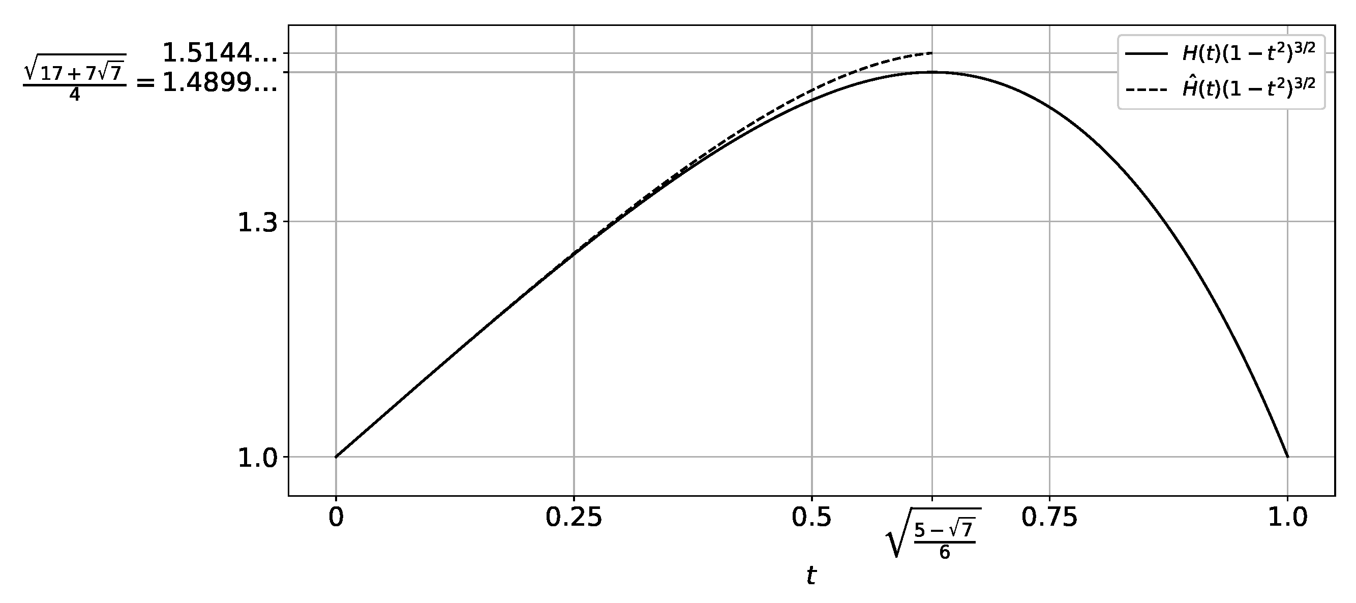
Figure 1. Plots of the functions p ( t ) and p ˜ ( t ) defined in (13) and (14), respectively.
Mathematics 11 00625 g001
Figure 2. Plots of the functions H ( t ) ( 1 t 2 ) 3 / 2 and H ^ ( t ) ( 1 t 2 ) 3 / 2 .
Mathematics 11 00625 g002
Figure 3. The graphs of the functions f ( x ) = | x 1 | 3 and g ( x ) = a + b x + c x 2 + d | x | 3 from Lemma 1 (left) and the graph of the difference f g (right) for u = 5 , v = 10 ( d > 0 ). The unique minimum point of g lies between the tangency points u and v.
Mathematics 11 00625 g003
Figure 4. Plots of the functions f ( x ) = | x 1 | 3 and g ( x ) = a + b x + c x 2 + d | x | 3 from Lemma 1 (left), and the plot of the difference f g (right) for u = 1 , v = 2 ( d < 0 ). The unique minimum point of g lies between the tangency points u and v. The maximum points lie to the left from u and to the right from v.
Mathematics 11 00625 g004
Figure 5. Plots of the functions f ( x ) = | x 1 | 3 and g ( x ) = a + b x + c x 2 + d | x | 3 from Lemma 1 (left), and the plot of the difference f g (right) for u = 0.5 , v = 3 ( d > 0 ). The unique minimum point of g lies between the tangency points u and v. Two more stationary points, the minimum and the maximum points, lie to the left of u.
Mathematics 11 00625 g005
Figure 6. The plot of the function g ( u ) = 4 u 1 u 2 3 u 2 1 .
Mathematics 11 00625 g006
Figure 7. Plots of the functions M 1 ( · , t ) for some t.
Mathematics 11 00625 g007
Figure 8. Plots of the function M 2 ( · , t ) for some t.
Mathematics 11 00625 g008
Table 1. The values of the functions H ( t ) , H ( t ) ( 1 t 2 ) 3 / 2 , C 0 ( t ) = 0.3031 · H ( t ) ( 1 t 2 ) 3 / 2 , and the mass p ( t ) of one of the atoms of the extreme distribution rounded up, for some t [ 0 , 1 ) .
t H ( t ) H ( t ) ( 1 t 2 ) 3 / 2 C 0 ( t ) p ( t )
011 0.3031 3 3 6
0.001 1.00111 1.00111 0.3035 0.2116
0.01 1.0108 1.0107 0.3064 0.21405
0.05 1.057 1.053 0.3192 0.22494
0.1 1.1225 1.1057 0.3352 0.23856
0.2 1.285 1.20871 0.3664 0.26593
0.3 1.5034 1.3051 0.3956 0.29365
0.4 1.805 1.3896 0.4212 0.32205
0.5 2.2392 1.4544 0.4409 0.35168
0.6 2.9067 1.4882 0.4511 0.38345
5 7 6 1 + 2 7 2 1 A 2 17 + 7 7 4 0.4517 5 7 6
0.7 4.04901 1.4747 0.447 0.41691
0.8 6.4739 1.3984 0.4239 0.44833
0.9 15.041 1.2457 0.3776 0.47783
1 + 1 0.3031 0.5
Disclaimer/Publisher’s Note: The statements, opinions and data contained in all publications are solely those of the individual author(s) and contributor(s) and not of MDPI and/or the editor(s). MDPI and/or the editor(s) disclaim responsibility for any injury to people or property resulting from any ideas, methods, instructions or products referred to in the content.

Share and Cite

MDPI and ACS Style

Makarenko, V.; Shevtsova, I. Delicate Comparison of the Central and Non-Central Lyapunov Ratios with Applications to the Berry–Esseen Inequality for Compound Poisson Distributions. Mathematics 2023, 11, 625. https://doi.org/10.3390/math11030625

AMA Style

Makarenko V, Shevtsova I. Delicate Comparison of the Central and Non-Central Lyapunov Ratios with Applications to the Berry–Esseen Inequality for Compound Poisson Distributions. Mathematics. 2023; 11(3):625. https://doi.org/10.3390/math11030625

Chicago/Turabian Style

Makarenko, Vladimir, and Irina Shevtsova. 2023. "Delicate Comparison of the Central and Non-Central Lyapunov Ratios with Applications to the Berry–Esseen Inequality for Compound Poisson Distributions" Mathematics 11, no. 3: 625. https://doi.org/10.3390/math11030625

APA Style

Makarenko, V., & Shevtsova, I. (2023). Delicate Comparison of the Central and Non-Central Lyapunov Ratios with Applications to the Berry–Esseen Inequality for Compound Poisson Distributions. Mathematics, 11(3), 625. https://doi.org/10.3390/math11030625

Note that from the first issue of 2016, this journal uses article numbers instead of page numbers. See further details here.

Article Metrics