Mathematical Model Assisted Six-Sigma Approach for Reducing the Logistics Costs of a Pipe Manufacturing Company: A Novel Experimental Approach

Abstract

This research addresses and analyzes the results of a six-sigma approach used to optimize the logistics costs of a pipe manufacturing company. Two mathematical models are developed for containers to control the company’s logistics. The Mathematical Programming Language (MPL) software is used to generate and solve these models. The results verify that the proposed mathematical models result in the company’s logistics improvement, especially in the DMAIC (define, measure, analyze, improve, and control) cycle by providing flexibility in choosing the most appropriate containers for logistics.

1. Introduction

The flow of products, services, and information across the supply chain must be properly planned, implemented, and controlled. In the current competitive environment, the performance of transport plays a crucial role in a company’s growth and survival. As a result, enhancing logistics procedures directly improves firm competitiveness. By eliminating logistics operations that do not add value to the products, and by cutting product delivery times to clients, it saves logistics costs and increases the satisfaction of all stakeholders [1].

Generally, mathematical models are used to find optimized solutions to transportation and logistics problems. For well-defined systems, mathematical models can be developed precisely; however, if the system is not well defined in its current state, then alternative approaches are adopted to identify the underlying problem. Considering this, six-sigma is mostly preferred because it includes effective statistical tools for predicting the accurate solutions of unknown variables; for instance, Beumjun et al. investigated a well-defined logistics system for supplying parts to a manufacturer distribution center (depot) and developed a mathematical model to reduce a supplier’s inventory holding and shipping costs [2]. Salema et al. developed a generalized model for a generic reverse logistics network considering capacity restrictions, multi-product management, product demand, and product return uncertainty. They used a mixed-integer formulation and standard branch-and-bound methods and applied the proposed solution to a real-world scenario [3]. A study by Goetschalckx et al. demonstrated how strategic global supply chain networks could be combined with allocating critical production–distribution centers, substantially reducing transfer costs. Considering the success of the methodologies reported in published literature, the presented research focused on developing two mathematical models for logistics improvement [4].

The presented analysis investigates how to decrease the logistical expenses of a pipe manufacturing company. The company’s system was poorly defined due to several flaws in its production operations, inventory system, logistics, and supply chain. As a result, the six-sigma methodology was utilized as a first approach to minimize logistics time and overall price. The main objective was to resolve the underlying challenges and enhance the logistics operations distribution network. Therefore, the six-sigma approach’s DMAIC (define, measure, analyze, improve, and control) cycle was applied, and two mathematical models were developed [5,6,7,8,9,10,11,12,13,14,15,16,17,18,19]. The first model determines whether the idle areas of the plant can be used as potential storage areas. The second model analyzed the optimized stacking sequence and layout of containers. Although the models were not complex, the novelty is in the use of mathematical modeling as the major improvement tool in the DMAIC approach of six-sigma. The potential of mathematical programming for the six-sigma projects was conceptually discussed in the literature, but published cases were limited to the response surface optimization and parameter setting stages [6,7,8]. The current paper presents a unique six-sigma application enhanced with mathematical programming in the improve phase to solve common problems in pipe manufacturing companies. The methodology, primary outcomes, proposed improvements, and reliability of the proposed models are discussed in the proceeding sections.

2. Methodology

The components of six-sigma and the DMAIC process for the manufacturing firm were aimed at minimizing the logistics costs. The potential improvements in the logistics system and the deployment processes are explained below. For the improvement phase of the DMAIC approach, the Mathematical Programming Language (MPL) was used to formulate and optimize the selected logistics problems.

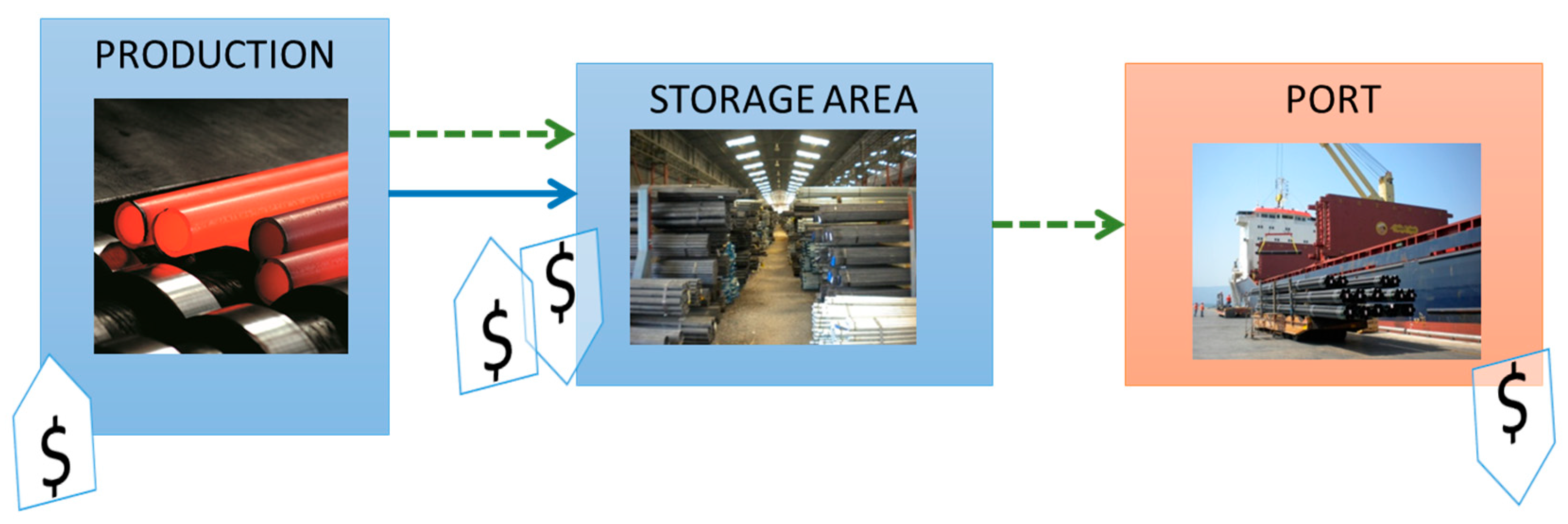
3. Modeling of the Logistics System

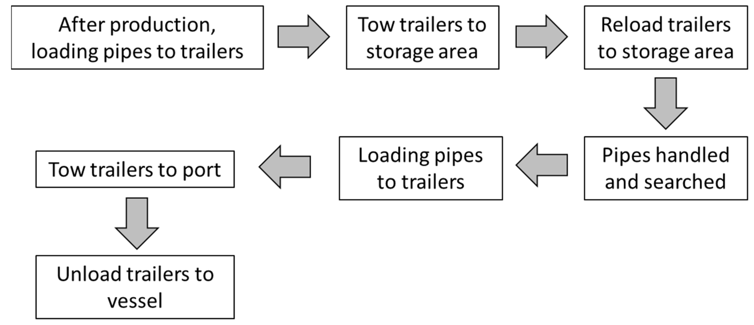
The annual production capacity of the firm contained 900,000 tons of pipes with various specifications. The sales department informs the production planning and control (PPC) department about the customer orders and specifications needed. The PPC then determines the expected completion time of orders. After an initial estimation, the vendors were consulted for the delivery dates of the vessels. These dates were critical for smooth loading operations and the avoiding of the extra costs for shipping companies in case of early arrivals. After the production of a lot, loading to the vessel was authorized, and pipes were transported by the first available vessel. Figure 1 describes the workflow process of the container loading and carrying operation.

The operations were based on the following limitations and assumptions:

(i).

Before the vessel arrives at the port, all production activities must be completed.

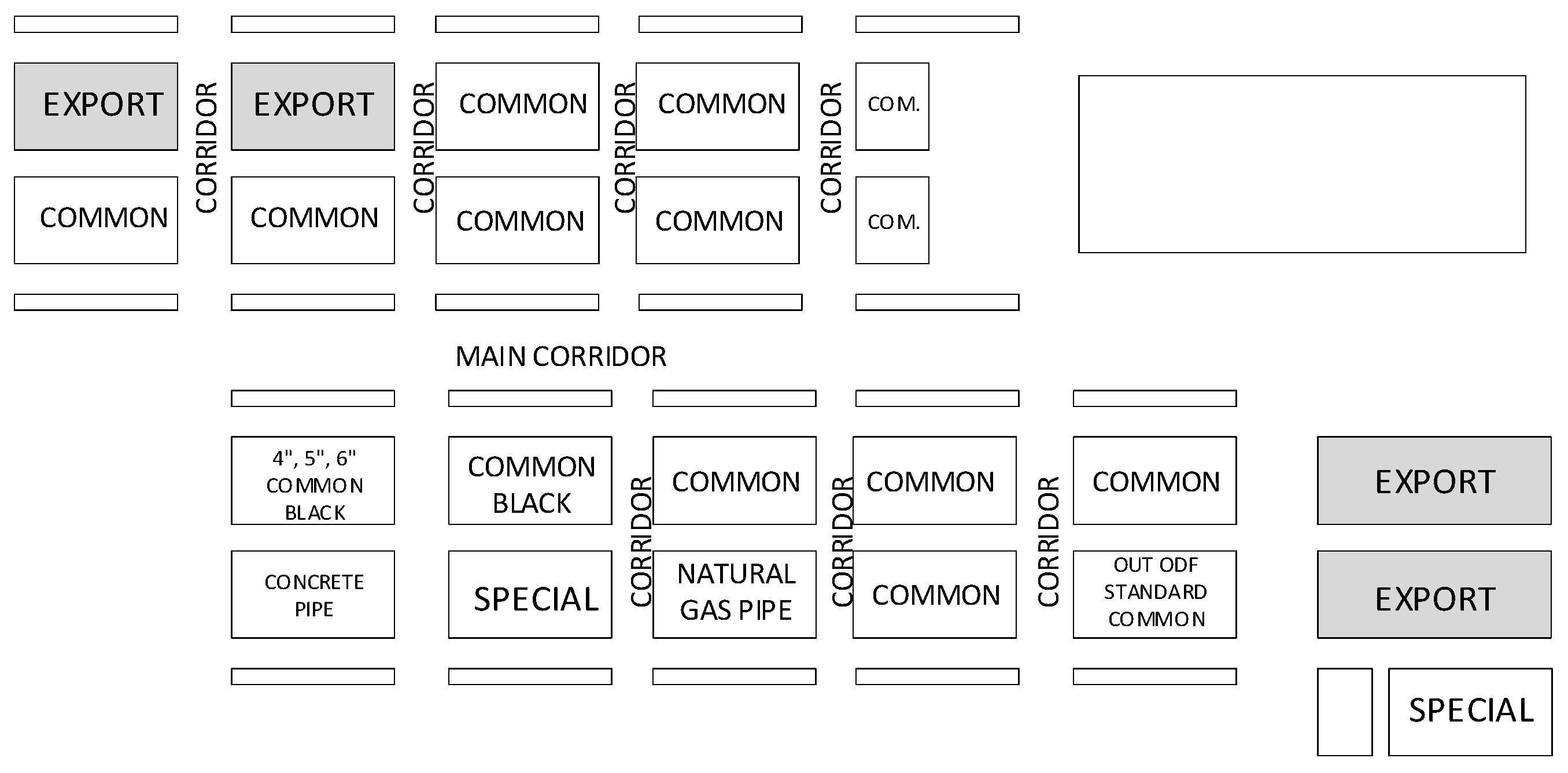
(ii).

If the designated storage area is insufficient, several types of pipes may be placed in other locations. This increases the company’s loading times and logistics costs.

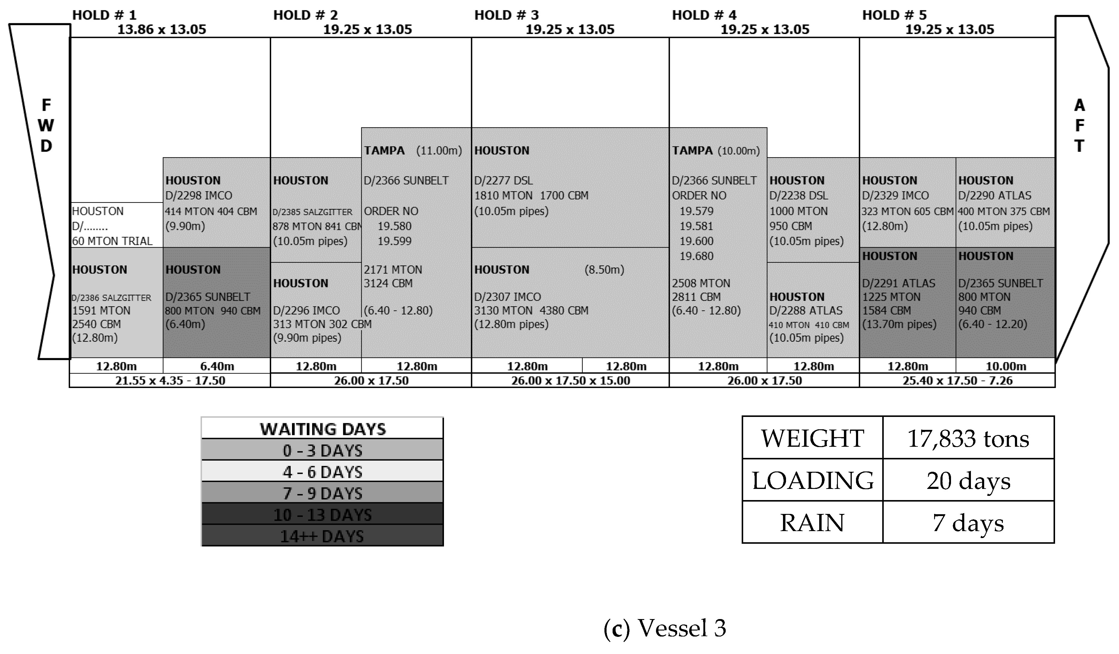
(iii).

The shape of the vessel hold affects the loading time and logistics costs. Loading into box-type holds is faster than other types of holds.

3.1. The DMAIC Cycle

3.1.1. Define Phase

The problems that arise in the vessel loading system are investigated during this phase. It was discovered that the current system had specific issues. For example, if loading times were long and loading costs were high due to unpredictable loading schedules, then the company was overcharged for these reasons [1]. Furthermore, if vessels remained idle over a certain period during the loading process, the company was obligated to pay an extra cost. Considering these factors, six-sigma is selected for the defined problem [1].

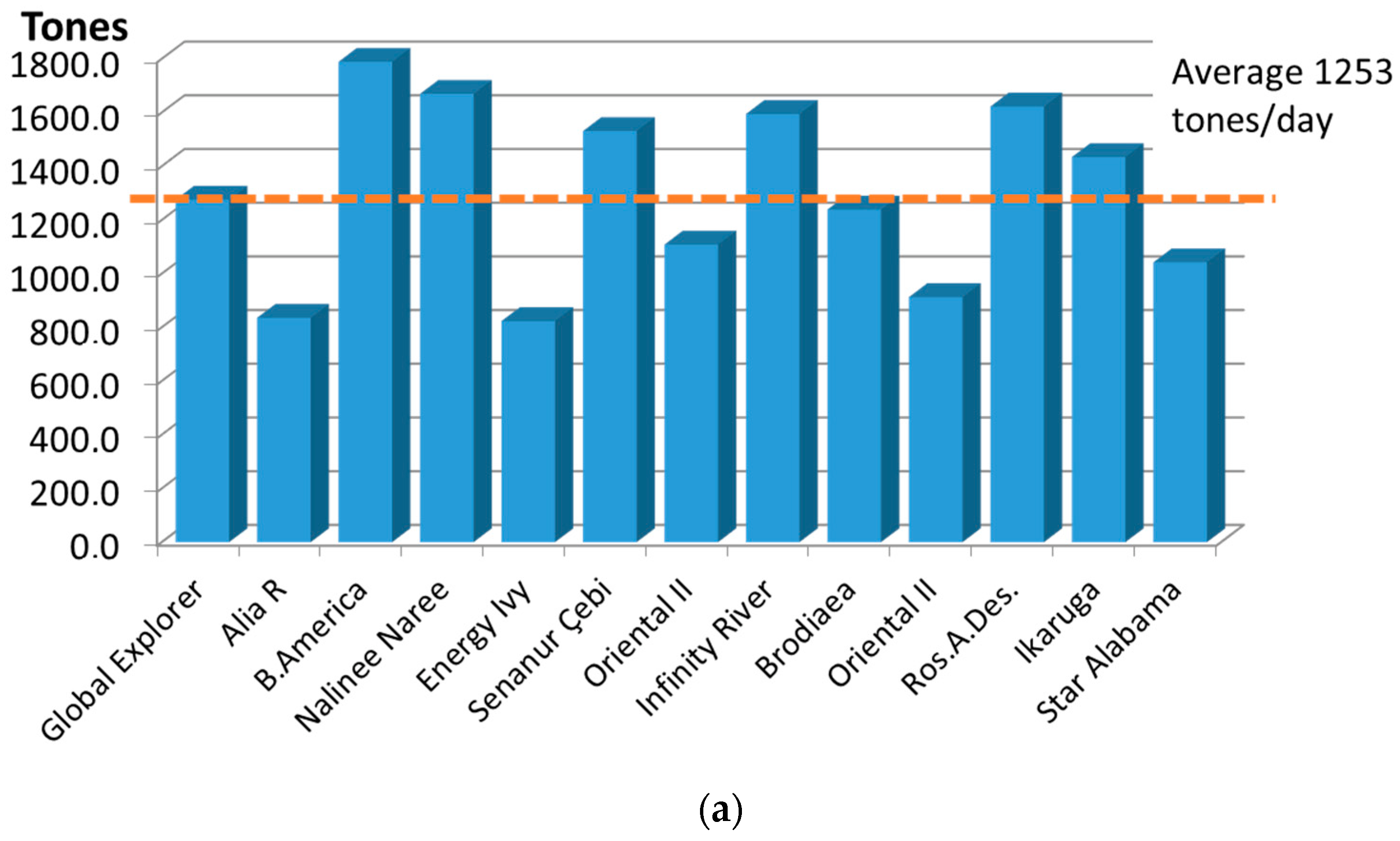
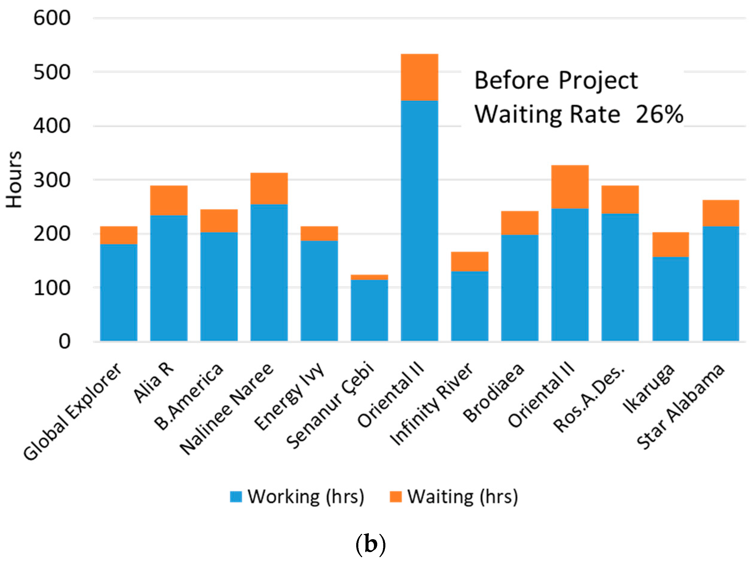
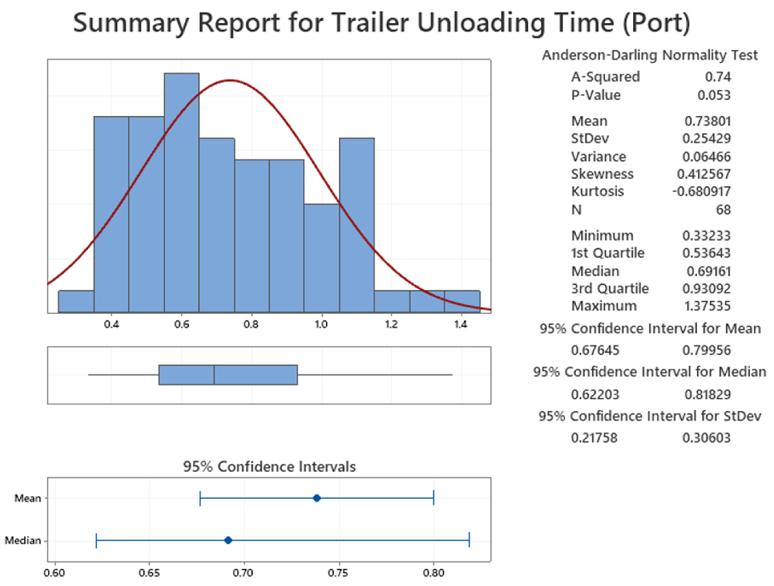
3.1.2. Measure Phase

The handling times in the storage area were investigated. The average daily rate of loading the vessel is 1253 tons, as shown in Figure 2a. Before the DMAIC, the average waiting time ratio was estimated to be 26%, as shown in Figure 2b. All of these values were averages for the years 2011–2021.

According to the average yearly loading reports of 2011–2021, the primary reason for waiting was the load waiting, as shown in Figure 3. Additionally, the other reasons were also considered in the analysis phase as they had the second most impact.

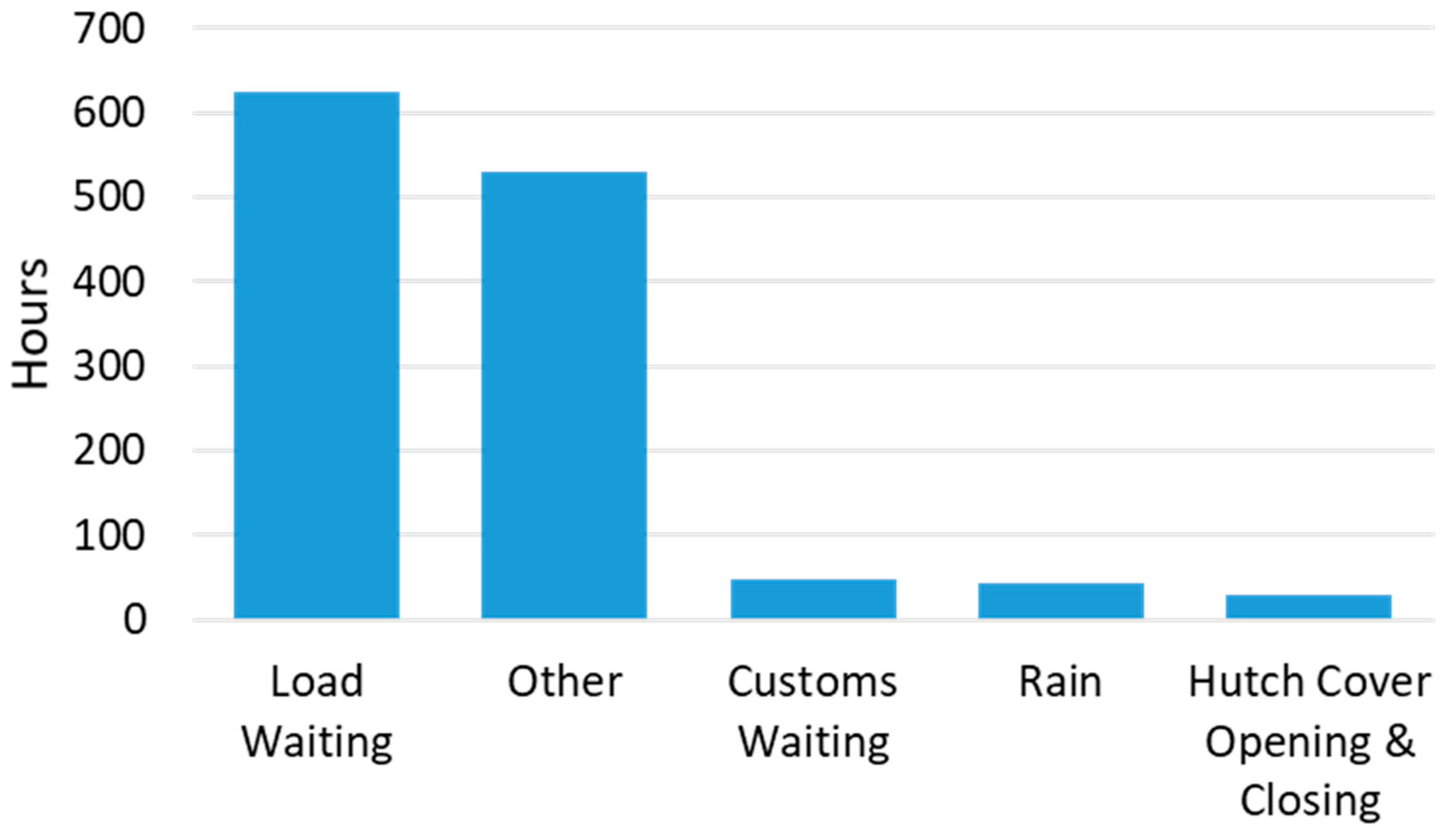
3.1.3. Analyze Phase

During the data analysis, four critical causes were identified that resulted in higher logistics time and cost, such as production tardiness, inefficient logistics process, inadequate storage area, and hard-to-load vessel designs. The following root causes of these critical causes were identified:

• Lack of communication between the manufacturing company’s departments of sales, production planning, production, and the vessel rental company
• Production delays due to the order sequencing problems
• Tardiness of production
• Inadequate deployment of lean production principles
• Limited daily vessel loading rate
• Low employee performance in the storage area and at the port
• Delayed logistics due to environmental issues

Figure 4 explains the completion of production in days for different types of pipes when various vessels arrive.

Trailer loading and unloading times for the selected trailers in the storage area and at the port were measured for estimated different parameters at the vessel loading operations. Minitab 19.0 was used for data analysis. The average loading time in the storage area was 51.214 min, and the standard deviation was 20.131 min, as shown in Figure 5. The average unloading time at the port was 31.765 min, and the standard deviation was 15.184 min, which can also be observed in Figure 6.

The storage area was originally planned for a total of 20,000 tons; however, the current weight of the pipes in the storage area was about 33,000 tons. Next, the loading and unloading time for packets was analyzed. It was determined that an average of 0.73097 packets per minute were loaded into the trailer in the storage area, as shown in Figure 7. In addition, it was determined that an average of 0.73801 packets per minute were loaded into the vessel at the port, as shown in Figure 8. The main objective was to eliminate the waiting time by keeping the loading rates equal on both sides. If one side’s rate is lower than the other, it causes a delay in the processing cycle of the other side.

3.1.4. Improve Phase

In the improvement phase, relevant solutions for each of the identified root causes were investigated. The availability of a solution and its deployment cost were the main concerns at this point. Therefore, the storage area has been properly organized. Production tardiness was a critical problem. This used to cause a significant delay in the vessel loading process. To solve this problem, monthly meetings were organized with participants from the sales, planning, and production departments and the vessel rental company. Even though the rental price of the vessels with box-type holds is higher, their selection is justified due to the time savings during the loading process.

The layout of the storage area was reorganized to solve the related problems. Since the company exports 75% of its production through the seaport, the pipes produced for the export market were assigned a higher priority in the storage area. In the current layout, all export market pipes were placed together; therefore, trailers could not operate simultaneously, meaning loading times were very high. To solve this problem, export market pipes were placed in four different sections of the storage area to allow the simultaneous loading of multiple trailers. The new layout is shown in Figure 9.

After incorporating these modifications, the efficiency of the logistics process increased. Vessel arrivals were not delayed because of the timely completed production runs. The new logistics system improved the three vessels’ loading performance. Before the DMAIC, the average daily loading rate was 1253 tons, and the average waiting time ratio was 26%. After implementing the DMAIC, the average daily loading rate was increased to 2470 tons while the average waiting time ratio was reduced to 13%. These improvements are displayed in Figure 10.

According to these results, the efficiency of the logistics system increased. The current average daily loading weights were doubled compared to the earlier practice. Additionally, the average waiting rate decreased by 50%. Additionally, only two types of cargo vessels were chosen for transportation, so one of the ships was eliminated. The company exceeded its target, which was 1800 tons/day, before implementing the DMAIC. The savings of the company were approximately $500,000 per year. Two other essential improvements for the company, due to using DMAIC, were the increased efficiency of the workers and deploying a lean six-sigma logistics system.

3.1.5. Control Phase

In this phase, the implementation of all changes was monitored. The waiting times and logistics costs were monitored. It was observed that the worker efficiency level increased and working conditions were improved.

Table 1. Part of control indicators and reactions.

Control Indicator	Level	Reaction
Vessel waiting time	Above 20 h	Check transportation ground vehicle schedule
Logistics cost	Above predetermined value	Check arriving vessel schedule and excess waiting times
Loaded pipes	Lower than 1800 tons	Check the ground transportation vehicle schedule
Worker efficiency	Lower than 80%	Check loading problems for both vessels and ground transportation

provides some relevant indicators in the control plan, including selected reactions.

3.2. Mathematical Models for Container Selection

For the improvement phase of the DMAIC problem, two mathematical models were developed to solve the storage-related issues. After observing an inadequate storage area, mathematical optimization was chosen as the primary approach. The first mathematical model aims to determine the types and numbers of containers with the minimum total cost. The option of storing the pipes in containers was considered when evaluating the unoccupied areas of the plant as storage areas. This option had the following benefits:

• Decreased pipe handling
• Increased daily vessel loading rate
• More flexible storage areas
• Open storage areas free of fixed cost
• Quadrupled quantity of pipes stored per square meter

One can observe the current logistic process in Figure 11, the logistic process with the container solution in Figure 12, and the new logistic process steps in Figure 13. In comparison, it is evident that the new logistic process is leaner and more efficient.

The layout of the areas on which the containers were to be placed is shown in Figure 14. The following issues were considered in the determination of the best location:

• Number of containers that can be placed in the area
• Ease of operation of the stackers
• Ease of removal of the containers
• Strength of the groundwork with a possibility of stacking up to 5 rows (for worker safety)

Figure 14. The layout of the areas to be used for storage.

Figure 14. The layout of the areas to be used for storage.

The container dimensions were standard (Figure 15), with a length of either 20 ft. or 40 ft. Properties of the containers in which the pipes were placed are given in

Table 2. Properties of the standard containers.

	20 ft. Container	40 ft. Container
Length (mm.) L1	5890	12,015
Height (mm.) H1	2400	2690
Width (mm.) B1	2345	2345
Unit prices ($)	3500	5000

(where L1 is the length, H1 is the height, and B1 is the width). The length of pipes includes 5, 8, 12, or 12.8 m. To determine the type of container selection for a particular scenario, a mathematical model was built with the following content:

At most, 14,000 tons of pipes were stored in the described area. Since five rows of containers were used, each row holds, at most, 2800 tons. A given type of pipe should be placed in a specific type of container. The company aims to limit the stock of each pipe by 1500 tons and to collocate pipe packages and place them in a line of 20 ft. Based on this information, the following mathematical model was developed.

Decision variables:

x_ij: Weight of type i pipe to be placed in type j container (in tons), i = 1,…,4, j = 1, 2.

y_ij: a binary variable which equals 1 if there is any type i pipe placed in type j container; 0, otherwise, i = 1,…,4, j = 1, 2.

Mathematical model:

$$\min 3500\left(\frac{x_{11}}{20}+\frac{x_{21}}{20}+\frac{x_{31}}{20}+\frac{x_{41}}{20}\right)+5000\left(\frac{x_{12}}{25}+\frac{x_{22}}{25}+\frac{x_{32}}{25}+\frac{x_{42}}{25}\right)$$

(1)

subject to

$$x_{11}\le 1500y_{11}$$

(2)

$$x_{12}\le 1500y_{12}$$

(3)

$$x_{21}\le 1500y_{21}$$

(4)

$$x_{22}\le 1500y_{22}$$

(5)

$$x_{31}\le 1500y_{31}$$

(6)

$$x_{32}\le 1500y_{32}$$

(7)

$$x_{41}\le 1500y_{41}$$

(8)

$$x_{42}\le 1500y_{42}$$

(9)

$$x_{11}+x_{12}+x_{21}+x_{22}+x_{31}+x_{32}+x_{41}+x_{42}=2800$$

(10)

$$y_{11}+y_{12}\le 1$$

(11)

$$y_{21}+y_{22}\le 1$$

(12)

$$y_{31}+y_{32}\le 1$$

(13)

$$y_{41}+y_{42}\le 1$$

(14)

$$\begin{gathered} 15\left(\frac{x_{11}}{20}+\frac{x_{21}}{20}+\frac{x_{31}}{20}+\frac{x_{41}}{20}\right)+30\left(\frac{x_{12}}{25}+\frac{x_{22}}{25}+\frac{x_{32}}{25}+\frac{x_{42}}{25}\right)\le 2700 \\ {x}_{ij}\ge 0, y_{ij}\in \left\{0,1\right\},i=1,\cdots ,4,j=1,2 \end{gathered}$$

(15)

Equation (1) defines the objective function, which tries to obtain the lowest total container-buying cost. Constraints 2–9 represent the weight that limits at most 1500 tons of pipe stored from each type. Constraint (10) defines the maximum amount of pipe in the storage area, which allows, at most, 2800 tons of pipes in each container row. Constraints (11 to 14) show that only a particular container can be used for a given type of pipe. Constraint (15) states that the available storage area is 2700 m², which can be occupied by the containers (45 m × 60 m).

The model was developed on the MPL (Mathematical Programming Language) platform and solved using the CPLEX 11.2.1 solver. The solution, summarized in

Table 3. The solution of the mathematical model for optimum container types.

Type of Pipe	Total Weight (Tons)	Preferred Container Type	Number of Containers	Cost ($)
1	1300	20 ft.	65	227,500
2	1500	20 ft.	75	262,500
			Total Cost	490,000

below, required less than a second on a Windows 10 installed PC with 8 GB of RAM and an AMD Ryzen 5 processor.

The company can economically determine the required number of containers by using the proposed model. The model is also beneficial due to its flexibility and accurate results [20,21,22].

The alignment of the containers in the storage area (45 m × 60 m × 13.5 m) was organized using a second mathematical model as described below.

The variables in the model include:

P, Q, R: length, width, and height of the storage area, respectively.

c_i, d_i, e_i: length, width, and height of the ith container, respectively.

Lx_i, ly_i, lz_i: binary variables that define the place of the ith container length according to the X, Y, and Z-axis, respectively.

wx_i, wy_i, wz_i: binary variables that define the place of the ith container width according to the X, Y, and Z-axis, respectively.

hx_i, hy_i, hz_i: binary variables that define the place of the ith container height according to the X, Y, and Z-axis, respectively.

x_i, y_i, z_i: front, left, and bottom points coordinates of the ith container, respectively.

The graphical representation of variables in the model can be observed in Figure 16.

The mathematical model is as below:

$$\mathrm{Max} {{\displaystyle \sum }}_i\left(\frac{45}{c_i}l{x}_i+\frac{45}{d_i}l{y}_i+\frac{45}{e_i}l{z}_i\right)+\left(\frac{60}{c_i}w{x}_i+\frac{60}{d_i}w{y}_i+\frac{60}{e_i}w{z}_i\right)+\left(\frac{13.5}{c_i}h{x}_i+\frac{13.5}{d_i}h{y}_i+\frac{13.5}{e_i}h{z}_i\right)$$

(16)

subject to

$${\displaystyle \sum }_i{c}_{i}l{x}_i+d_{i}w{x}_i\le P$$

(17)

$${\displaystyle \sum }_i{c}_{i}l{y}_i+d_{i}w{y}_i\le Q$$

(18)

$${\displaystyle \sum }_i{c}_{i}l{z}_i+d_{i}w{z}_i\le R$$

(19)

$$l{x}_i+l{y}_i+l{z}_i=1, \forall i$$

(20)

$$w{x}_i+w{y}_i+w{z}_i=1, \forall i$$

(21)

$$h{x}_i+h{y}_i+h{z}_i=1, \forall i$$

(22)

$$l{x}_i+w{x}_i+h{x}_i=1, \forall i$$

(23)

$$l{y}_i+w{y}_i+h{y}_i=1, \forall i$$

(24)

$$l{z}_i+w{z}_i+h{z}_i=1, \forall i$$

(25)

$$l{z}_i=0, \forall i$$

(26)

$$w{z}_i=0, \forall i$$

(27)

$$h{z}_i=1, \forall i$$

(28)

The objective function defined by Equation (16) aims to maximize the number of containers placed in the storage area. Constraints (17–19) are storage area constraints. These constraints ensure containers are not placed outside of the storage area. Constraints (20–25) ensure that only one edge of the containers is parallel to one of the edges of the storage area. Constraints (26–28) are unique to our model. With these constraints, we ensure that the container’s vertical axis is perpendicular to the ground.

The model is linear since c_i, d_i, and e_i are all constants. In our application, the dimensions of the containers were 13.555 m × 2.348 m × 2.695 m. Since the containers were only placed on their bases, we could concentrate on the remaining two planar dimensions. Dividing the height of the storage by the height of the standard container, we see that it is possible to stack 5 (≅13.5/2.695) layers of containers.

The reduced model was also coded in MPL and solved using CPLEX 11.2.1 in less than a second on a Windows 10 installed PC with 8 GB of RAM and an AMD Ryzen 5 processor. The model shows how many identical lines of containers can be placed along both the X and Y axes. The optimal solution results indicate that the axis of Y is binding with six lines of containers while there is still some room for extra lines of containers, as shown in

Table 4. The solution of the mathematical model for storage area optimization.

Line (i)	lxi	lyi
1	0	1
2	0	1
3	0	1
4	0	1
5	1	0
6	1	0

.

The slacknesses in both directions were calculated as follows:

X-axis: 45−4 ∗ 2.348−2 ∗ 13.555 = 8.498 m,

Y-axis: 60−4 ∗ 13.555−2 ∗ 2.348 = 1.084 m.

Since the model locates a set of standard lines of containers in the storage area, the remaining areas were left to be manually organized, as seen in

Table 5. Detailed layout storage area.

Section of the Storage	Number of Horizontal Lines	Number of Horizontal Lines	Number of Containers	Area (m2)
1	4	4	16	509.23
2	2	23	46	1464.05
3	3	2	6	190.96
4	3	4	12	381.93
		Sum	80	2546.17

.

Results show that we achieve an area utilization of 94.3% since the total floor area is 2700 (=60 × 45) m². Meanwhile, we can fit 80 containers in each layer; this also shows that we use 95.24% (=80/84) of the theoretical capacity in units of containers to be calculated by dividing the floor area by the container base area (84 = 2700/(13.555 × 2.348).

4. Identified Gaps and Directions for Future Research

In the six-sigma literature, one of the most critical gaps we noticed was the underutilization of mathematical optimization in the improvement phase. Therefore, this paper humbly aims to fill out some aspects of this gap. In our trial, to enhance the improvement phase by mathematically formulating and solving the involved decision problems, we tackled the issues of how to determine the best container types for the pipes and how to align these containers in the storage area. The problems and data were specific to the company studied for this case. The formulations need to be revised accordingly when applied in different settings. For example, in the first model for determining the container types with minimum cost, the geometric definitions of pipes, potential containers, and the cost data should be identified beforehand for the local practice. In the second model, in which we aim to utilize the space of the storage zone better, the types and numbers of the containers determined by using the first model and the geometric specifications of the storage zone were the inputs to be appropriately set according to the local case. Hence, the mathematical models were directly related to the problems which have been observed during the six-sigma process. Their contents were considered as is without simplifying or complicating any components. The models were originally within the solution capabilities of a widely used mathematical optimization software. Therefore, neither the problem content nor the solution process was beyond the current knowledge base. However, the originality of this paper comes from the advantage of mathematical optimization within the practice of the six-sigma approach. By integrating the mathematical optimization into the improvement phase of six-sigma (DMAIC) projects, we will be able to obtain the combined benefit of two individually practiced approaches such as mathematical optimization and process improvement.

The models can be employed in similar settings after parametric adjustments. However, there may be a need for a redefinition of decision variables and constraints when there is a possibility of freely using the third dimension in the bin packing problem. We were able to take advantage of presetting the third dimension since only the same product containers were to be stacked in our case. A recent literature survey on two- and three-dimensional packing problems can be seen before making efforts to develop a mathematical model for the applicable problem [20,23,24]. These changes are appended to the manuscript in its final form.

There are many other issues to be covered in a typical pipe manufacturing company’s logistics processes using mathematical optimization. Additionally, there was no formal or methodological sigma-level calculation for the transportation of pipes in the literature [25,26,27]. The vessels’ standard loading/unloading times can be considered a control variable, and the sigma level can be calculated accordingly. An additional research area to be explored in this company may be the optimal scheduling of the vehicles transporting the pipes from the factory to the storage area and from the storage area to the port. These issues can be a-ddressed in future related research [28,29].

5. Conclusions

In this study, the six-sigma methodology was employed to lower a pipe manufacturing company’s logistics cost; as a result, the DMAIC cycle approach was adopted step by step. For the DMAIC approach’s improvement phase, the firm’s logistics system was first examined, then its core problems were recognized and solved systematically. For further improvements, two mathematical models were developed and solved using the MPL software to evaluate the open areas in the plant as potential storage areas [30].

As a result of all these improvements, total outbound logistics time was reduced considerably, and loading capacity was doubled compared to the earlier case. The company continues to address the feasibility of the new logistics system with containers supported by the results of this combined approach of six-sigma and mathematical optimization.

References

1. Küçük, M.; Orbak, A.Y. Six Sigma Approach for the Reduction of Transportation Costs of a Pipe Manufacturing Company. In Proceedings of the 2011 IEEE International Conference on Quality and Reliability, ICQR, Bangkok, Thailand, 11–14 September 2011; pp. 541–545. [Google Scholar]
2. Beumjun, A.; Watanabe, N.; Hiraki, S. A Mathematical Model to Minimize the Inventory and Transportation Costs in the Logistics Systems. Comput. Ind. Eng. 1994, 27, 229–232. [Google Scholar]
3. Salema MI, G.; Poboa AP, B.; Novais, A.Q. An optimization model for the design of a capacitated multi-product reverse logistics network with uncertainty. Eur. J. Oper. Res. 2005, 179, 1063–1077. [Google Scholar] [CrossRef]
4. Goetschalckx, M.; Vidal, C.J.; Dogan, K. Modeling and design of global logistics systems: A review of integrated strategic and tactical models and design algorithms. Eur. J. Oper. Res. 2001, 143, 1–18. [Google Scholar] [CrossRef]
5. Barney, M. Motorola’s second generation. Six Sigma Forum Mag. 2002, 1, 13–16. [Google Scholar]
6. Tang, L.C.; Goh, T.N.; Lam, S.W.; Zhang, C.W. Fortification of Six Sigma: Expanding the DMAIC Toolset. Qual. Reliab. Eng. Int. 2007, 23, 3–18. [Google Scholar] [CrossRef]
7. De Mast, J.; Lokkerbol, J. An analysis of the Six Sigma DMAIC method from the perspective of problem solving. Int. J. Prod. Econ. 2012, 139, 604–614. [Google Scholar] [CrossRef]
8. Stanivuk, T.; Gvozdenovic, T.; Mikulicic, J.Z.; Lukovac, V. Application of Six Sigma Model on Efficient Use of Vehicle Fleet. Symmetry 2020, 12, 857. [Google Scholar] [CrossRef]
9. Harry, M.J.; Schroeder, R. Six Sigma: The Breakthrough Management Strategy Revolutionizing the World’s Top Corporations; Doubleday: New York, NY, USA, 2002; Chapter 1. [Google Scholar]
10. Godfrey, A.B. The Honeywell Edge. In Six Sigma Forum Magazine; ASQ: Milwaukee, WI, USA, 2002; Volume 1, pp. 14–17. [Google Scholar]
11. Slater, R. Jack Welch and the GE Way: Management Insights and Leadership Secrets of the Legendary CEO; McGraw-Hill: New York, NY, USA, 1999; Chapter 1. [Google Scholar]
12. Kwak, Y.H.; Anbari, F.T. Benefits, obstacles, and future of six sigma approach. Technovation 2004, 26, 708–715. [Google Scholar] [CrossRef]
13. McClusky, R. The rise, fall, and revival of six sigma. Meas. Bus. Excell. 2000, 4, 6–17. [Google Scholar]
14. Brady, J.E.; Allen, T.T. Six sigma literature: A review and agenda for future research. Qual. Reliab. Eng. Int. 2005, 22, 335–367. [Google Scholar] [CrossRef]
15. Aksoy, B.; Orbak, A.Y. Reducing the Quantity of Reworked Parts in a Robotic Arc Welding Process. Qual. Reliab. Eng. Int. 2009, 25, 495–512. [Google Scholar] [CrossRef]
16. Forcina, A.; Silvestri, L.; Di Bona, G.; Silvestri, A. Reliability allocation methods: A systematic literature review. Qual. Reliab. Eng. Int. 2020, 36, 2085–2107. [Google Scholar] [CrossRef]
17. Özlem, E.; Kuyzu, G.; Savelsberg, M. Reducing Truckload Transportation Costs Through Collaboration. Transp. Sci. 2007, 41, 206–221. [Google Scholar]
18. Chen, C.S.; Lee, S.M.; Shen, Q.S. An Analytical Model for the Container Loading Problem. Eur. J. Oper. Research 1995, 80, 68–76. [Google Scholar] [CrossRef]
19. Küçük, M. Improvement of Logistics Processes of a Factory that Produces Steel Pipe. Master’s Thesis, Bursa Uludağ University, Graduate School of Natural and Applied Sciences, Industrial Engineering Department, Bursa, Türkiye, 2013. [Google Scholar]
20. Ali, S.; Ramos, A.G.; Carravilla, M.A.; Oliveira, J.F. On-line three-dimensional packing problems: A review of off-line and on-line solution approaches. Comput. Ind. Eng. 2022, 168, 108122. [Google Scholar] [CrossRef]
21. Liu, Z.; Wang, Y.; Feng, J. Vehicle-type strategies for manufacturer’s car sharing. Kybernetes 2022. ahead-of-print. [Google Scholar] [CrossRef]
22. Di Bona, G.; Cesarotti, V.; Arcese, G.; Gallo, T. Implementation of Industry 4.0 technology: New opportunities and challenges for maintenance strategy. Procedia Comput. Sci. 2021, 180, 424–429. [Google Scholar] [CrossRef]
23. Ye, R.; Liu, P.; Shi, K.; Yan, B. State Damping Control: A Novel Simple Method of Rotor UAV With High Performance. IEEE Access 2020, 8, 214346–214357. [Google Scholar] [CrossRef]
24. Wu, H.; Jin, S.; Yue, W. Pricing Policy for a Dynamic Spectrum Allocation Scheme with Batch Requests and Impatient Packets in Cognitive Radio Networks. J. Syst. Sci. Syst. Eng. 2022, 31, 133–149. [Google Scholar] [CrossRef]
25. Zheng, H.; Jin, S. A Multi–Source Fluid Queue Based Stochastic Model of the Probabilistic Offloading Strategy in a MEC System with Multiple Mobile Devices and a Single MEC Server. Int. J. Appl. Math. Comput. Sci. 2022, 32, 125–138. [Google Scholar] [CrossRef]
26. Wang, Y.; Han, X.; Jin, S. MAP based modeling method and performance study of a task offloading scheme with time-correlated traffic and VM repair in MEC systems. Wirel. Netw. 2023, 29, 47–68. [Google Scholar] [CrossRef]
27. Shao, Z.; Zhai, Q.; Han, Z.; Guan, X. A linear AC unit commitment formulation: An application of data-driven linear power flow model. Int. J. Electr. Power Energy Syst. 2023, 145, 108673. [Google Scholar] [CrossRef]
28. Tripathi, V.; Chattopadhyaya, S.; Mukhopadhyay, A.K.; Sharma, S.; Li, C.; Di Bona, G. A Sustainable Methodology Using Lean and Smart Manufacturing for the Cleaner Production of Shop Floor Management in Industry 4.0. Mathematics 2022, 10, 347. [Google Scholar] [CrossRef]
29. Silvestri, L.; Forcina, A.; Di Bona, G.; Silvestri, C. Circular economy strategy of reusing olive mill wastewater in the ceramic industry: How the plant location can benefit environmental and economic performance. J. Clean. Prod. 2021, 326, 129388. [Google Scholar] [CrossRef]
30. Silvestri, C.; Silvestri, L.; Forcina, A.; Di Bona, G.; Falcone, D. Green chemistry contribution towards more equitable global sustainability and greater circular economy: A systematic literature review. J. Clean. Prod. 2021, 294, 126137. [Google Scholar] [CrossRef]
Figure 1. The vessel loading process.
Mathematics 11 00621 g001
Figure 2. (a) Average daily loading rate (before) and (b) Average waiting rate (before).
Mathematics 11 00621 g002aMathematics 11 00621 g002b
Figure 3. Waiting time and delays (average of years 2011–2021).
Mathematics 11 00621 g003
Figure 4. Completion of production in days for different types of pipes when (a) Vessel 1 arrives, (b) Vessel 2 arrives, and (c) Vessel 3 arrives.
Mathematics 11 00621 g004aMathematics 11 00621 g004b
Figure 5. Average loading time in the storage area.
Mathematics 11 00621 g005
Figure 6. Average unloading time at the port.
Mathematics 11 00621 g006
Figure 7. Trailer loading performance in the storage area.
Mathematics 11 00621 g007
Figure 8. Trailer unloading performance at the port.
Mathematics 11 00621 g008
Figure 9. New storage area layout.
Mathematics 11 00621 g009
Figure 10. (a) Average daily loading rate (after), and (b) Average waiting rate (after).
Mathematics 11 00621 g010
Figure 11. Current logistics process.
Mathematics 11 00621 g011
Figure 12. The logistic process with a container solution.
Mathematics 11 00621 g012
Figure 13. New logistic process steps.
Mathematics 11 00621 g013
Figure 15. Standard container measurements.
Mathematics 11 00621 g015
Figure 16. Graphical representation of variables in the model.
Mathematics 11 00621 g016