Article

Outlier Detection of Crowdsourcing Trajectory Data Based on Spatial and Temporal Characterization

1
Department of Traffic Information and Control Engineering, Jilin University, Changchun 130022, China
2
College of Navigation, Jimei University, Xiamen 361021, China
*
Author to whom correspondence should be addressed.
Mathematics 2023, 11(3), 620; https://doi.org/10.3390/math11030620
Submission received: 18 December 2022 / Revised: 19 January 2023 / Accepted: 24 January 2023 / Published: 26 January 2023

Abstract

:
As an emerging type of spatio-temporal big data based on positioning technology and navigation devices, vehicle-based crowdsourcing data has become a valuable trajectory data resource. However, crowdsourcing trajectory data has been collected by non-professionals and with multiple measurement terminals, resulting in certain errors in data collection. In these cases, to minimize the impact of outliers and obtain relatively accurate trajectory data, it is crucial to detect and clean outliers. This paper proposes an efficient crowdsourcing trajectory outlier detection (CTOD) method that detects outliers from the trajectory sequence data in both spatial view and temporal view. Specifically, we first use the adaptive spatial clustering algorithm based on the Delaunay triangulation (ASCDT) algorithm to remove the location offset points in the trajectory sequence. After that, based on the most basic attributes of the trajectory points, a 6-dimensional movement feature vector is constructed for each point as an input. The feature-rich trajectory sequence data is reconstructed using the proposed temporal convolutional network autoencoder (TCN-AE), and the Squeeze-and-Excitation (SE) channel attention mechanism is introduced. Finally, the effectiveness of the CTOD method is experimentally verified.

1. Introduction

As an emerging type of spatio-temporal big data based on positioning technology and navigation devices, vehicle-based crowdsourcing data has become a valuable trajectory data resource. The analysis and mining of spatio-temporal trajectory data is fundamental content in the field of urban management and human activity, which consists of trajectory clustering [1], trajectory correlation analysis [2], trajectory prediction [3], target motion pattern recognition [4], and outlier detection [5], etc. However, crowdsourcing trajectory data is collected by non-professionals and multiple measurement terminals, resulting in some errors in the data collection. In these cases, the points in the trajectory that have significant inconsistencies with most of their neighbors are called outliers. To minimize the impact of outliers and obtain relatively accurate trajectory data, detecting and cleaning outliers is a crucial task.
Since vehicles are constrained by the road network and traffic rules in the real world, most of the trajectory points are located on the road surface. Only a tiny proportion of the trajectory points offset beyond the road edge line because of vegetation, buildings, and other factors [6]. Under this premise, researchers have attempted to use the method of spatial clustering to eliminate the trajectory points in the low-density region [7,8]. For example, Wang [9] adopted a kernel density function to remove outliers with low spatial density. While density clustering can only eliminate offset points, it cannot eliminate the low precision trajectory points in the high-density region. To solve this problem, some studies have considered the movement characteristics of the trajectory points. For instance, Yang [10] proposed a partition-and-filter model for filtering trajectories, which divides trajectories based on distance and angle constraints, and then filters sub-trajectories according to the desired trajectory-filtering accuracy. All of the above methods require massive manual testing to adjust the parameters. Furthermore, the detection performance is highly dependent on the accuracy of the parameters and cannot automatically learn the differences between the abnormal and normal data.
In recent research, machine learning and deep learning methods, which can automatically learn features from big data, have shown more significant potential for the outlier detection task. Among machine learning models, support vector machines (SVM) [11,12], local outlier factors (LOF) [13,14], and isolation forests (IF) [15] are widely used for outlier detection. Choi [11] proposed a modified SVM that weights feature vectors to reflect the local density of the support vectors and quantify classification uncertainty in terms of the local classification capability of each training sample. Degirmenci [13] proposed RiLOF, based on LOF, which has a high detection rate even in high-dimensional data; Mansoor [15] developed an outlier detection technique named “iF_Ensemble” for a Wi-Fi indoor localization environment. These proposed machine learning methods offer good accuracy with small datasets, but those with shallow learning networks perform unsatisfactorily with large-scale datasets.
In contrast, deep learning methods are more effective. Mahmoud [16] combined Convolutional Neural Networks (CNNs) and Long Short Term Memory Networks (LSTMs) to capture the spatio-temporal characteristics of network traffic and has higher detection accuracy than individual models. Canizo [17] proposed a novel Multi-head CNN-RNN architecture for multi-sensor time series outlier detection, which extracts the features of each sensor separately. Even though the above methods provide better results, they require a large amount of labeled data for training, and the accessible labeled data is usually limited.
For this reason, unsupervised outlier detection methods based on deep learning have gained wide popularity recently. For example, Autoencoder (AE) [18] performs outlier detection by examining its reconstruction loss. Yao [19] applied Variational Autoencoder (VAE) to extract valuable features for the unsupervised outlier detection tasks. However, the above methods are effective only when applied to non-serial data and not when applied directly to time series data. Since it treats each data block as a separate input while a trajectory is a sequence of points related to spatial and temporal information, modeling data blocks as separate vector inputs results in a loss of correlation. Provotar [20] proposed a Short-Term Long Memory-based Autoencoders network (LSTM-AE) to detect internet routing outliers. The LSTM memory units are used instead of ordinary neurons to build the coder for historical-study time series modeling. The problem is that LSTM requires a large amount of memory for long-time sequences to store cell states.
Nevertheless, all the aforementioned methods are only based on the spatial proximity among trajectory points or the temporal evolutionary nature of trajectory sequences for outlier detection, and none of them provides a complete solution to the problem of outlier detection. Therefore, this paper proposes a two-phase crowdsourcing trajectory outlier detection framework (CTOD) that combines both spatial perspective and temporal perspective, including spatial outlier detection phase and temporal outlier detection phase. During the spatial outlier detection phase, to remove the location offset point in trajectory sequences, we introduce the adaptive spatial clustering algorithm based on the Delaunay triangulation (ASCDT) algorithm of Deng, Liu, Cheng, and Shi [21]. During the temporal outlier detection phase, to enrich the input features, we first construct a 6-dimensional movement feature vector for each point as input to the model. Subsequently, we use the Temporal Convolutional Network Autoencoder (TCN-AE) model to identify temporal correlations between trajectory sequences, and remove movement property outliers by comparing the reconstruction loss of each trajectory point with a given outlier threshold. Specifically, we add the Squeeze-and-Excitation (SE) channel attention mechanism to enhance the feature extraction capability of the TCN. The contributions of this paper are summarized below.
  • We discuss and categorize common problems in crowdsourcing trajectory points, including trajectory point offsets that may be caused by navigation device errors or significant inconsistencies in trajectory point movement features due to acquisition process errors.
  • We present two trajectory outlier definitions, including Location Offset Points (LO-outlier) and Movement Property outliers (MP-outlier).
  • We propose a two-phase trajectory outlier detection framework (denoted as CTOD) to identify both types of trajectory outliers.
  • We conduct a comprehensive experiment on a real-world vehicle trajectory dataset to manifest the effectiveness and superiority of our approach compared with other congeneric approaches.
This article is structured as follows: Section 1 introduces the research background and reviews the related work in the literature. In Section 2, we define the classification of trajectory outliers and discuss the challenging problems in trajectory outlier detection. Section 3 outlines the scheme and elaborates the details of the CTOD model. Section 4 evaluates the proposed method. Section 5 concludes the whole article and point out future directions.

2. Preliminaries

2.1. Classification of Crowdsourcing Trajectory Outliers

Crowdsourcing trajectory data is derived from many contributors, and the accuracy of the navigation devices used by each contributor also varies, resulting in inaccurate, incomplete, and illogical data in the trajectories. In this paper, trajectory outliers are classified into two categories.
Location Offset Points (LO-outliers). The recorded trajectory data may produce a location deviation when a mobile object is in a weak signal area, such as in tunnels, under tall buildings, or when the navigation device has low positioning accuracy. Trajectory points may offset outside the road due to the location deviation, causing serious inconsistencies with neighboring points ( P 3 , P 4 in Figure 1).
Movement Property outliers (MP-outliers). In the process of collecting, transmitting, storing, and processing trajectory data, errors are generated by humans and instruments. These errors can result in significant differences in the movement properties between trajectory points, such as speed, direction, or other attributes.

2.2. Challenges in Trajectory Outlier Detection

While the outlier detection method for trajectory big data has been thoroughly investigated, it remains challenging due to localization uncertainties, uneven distribution area, skewed distribution, and large scale.
The challenges are as follows:
  • In general, LO-outliers have a lower point density than those inside the roads. Additionally, since trajectory points are distributed unevenly, some points inside the roads with sparse points also have a low point density, causing these points to be removed as LO-outliers.
  • Trajectory contributors use various navigation devices, which causes differences in the attribute categories. Some trajectory data collect attributes such as velocity and direction angle for each point, but some trajectory data only collect coordinates and time stamps. It is challenging to extract multidimensional movement features based on limited attributes.
  • Trajectories are spatial sequences generated over time, so there is a spatial and temporal correlation between trajectory points. To mine the temporal correlation implied, it is necessary to explore the association between the independent movement features of the points within the trajectory. Moreover, since different movement features contribute differently to the temporal correlation extraction, extracting representative movement features for each trajectory point is challenging.

3. Framework: Spatial and Temporal Outlier Detection in Trajectory Data

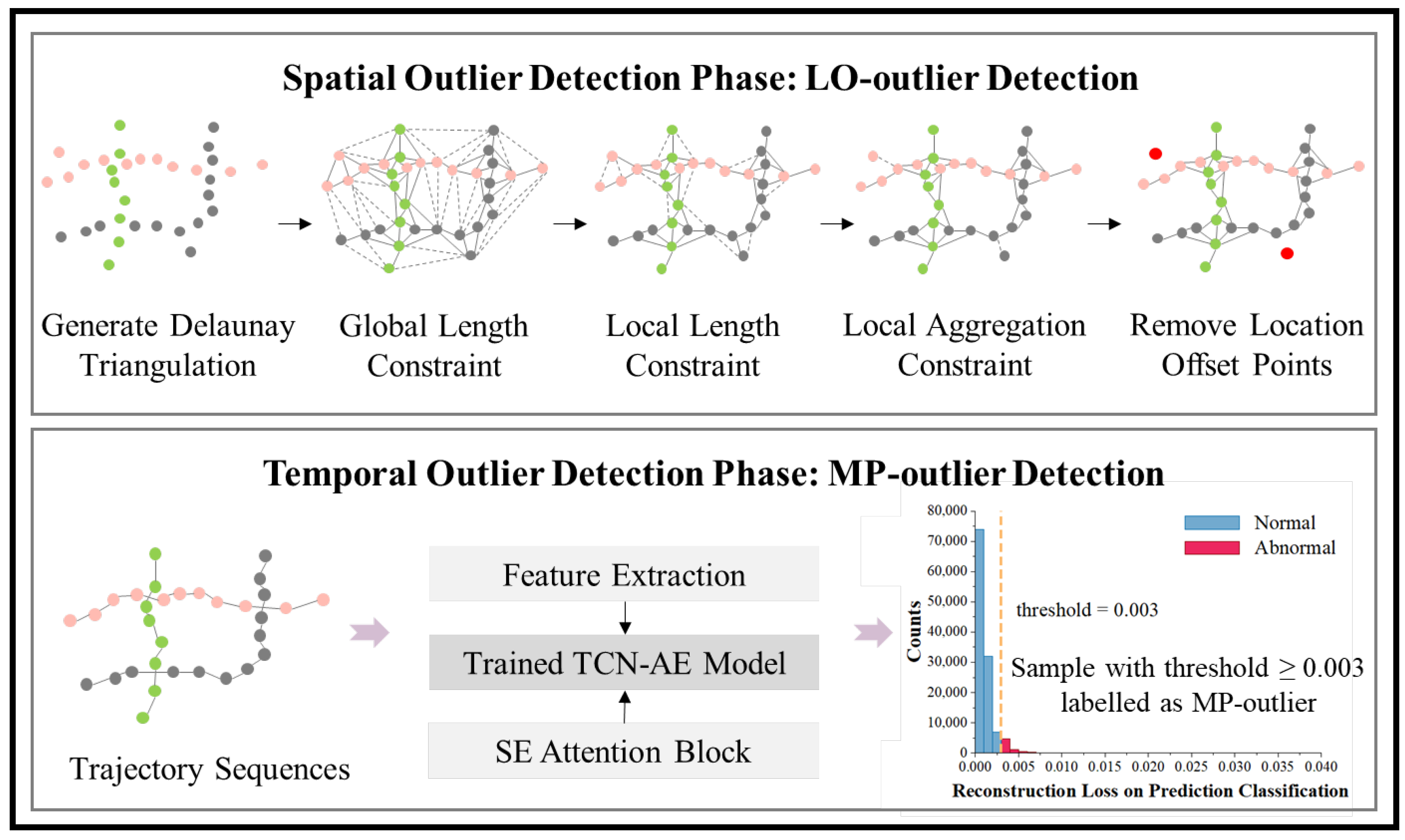
In this section, we propose a two-phase framework including a spatial outlier detection phase and temporal outlier detection to identify LO-outliers and MP-outliers, respectively (Figure 2. Framework of CTOD).

3.1. Spatial Outlier Detection Phase: LO-Outlier Detection

During the spatial outlier detection phase, the ASCDT algorithm based on Delaunay triangulation is introduced to identify LO-outliers and tackle Challenge 1 presented in Section 2. First, we construct spatial topotaxy among the spatial points, which generates triangle meshes by connecting sampling points. Further, the inconsistent edges are removed from the Delaunay triangulation by constraining the length of the edges and the aggregation force of the spatial points. As a result, the points without edges connected to them are identified as outliers. Therefore, identifying and removing these inconsistent edges is the key to separating outliers.

3.1.1. Delaunay Triangulation Generation

Given a set of spatial points S = P 1 , P 2 , , P n in a 2-dimensional space, let DT(S) be the Delaunay triangulation of S where each point P i represents a vertex. The necessary and sufficient condition of the Delaunay triangulation is that no point of S is in the circumcircle of any triangle in the triangulation.

3.1.2. Global Length Constraint in Delaunay Triangulation

For each point P i , the global length constraint can be represented as
G l o b a l _ L e n g t h _ C o n s t r a i n t P i                                                                 = G l o b a l _ M e a n D T + α G l o b a l _ V a r i a t i o n D T
α = G l o b a l _ M e a n D T / L o c a l _ M e a n P i
where G l o b a l _ M e a n D T is the mean length of the edges in the Delaunay triangulation, L o c a l _ M e a n P i is the mean length of the edges in relation to P i , and Global _ Variation D T is the standard deviation of the length of all edges in the Delaunay triangulation.
The edge e j directly connected to a point P i in Delaunay triangulation, which has a length larger than or equal to G l o b a l _ L e n g t h _ C o n s t r a i n t P i , will be categorized to G l o b a l _ L o n g _ E d g e s and removed from the Delaunay triangulation at a global level. Otherwise, if e j has a length shorter than G l o b a l _ L e n g t h _ C o n s t r a i n t P i , it will be categorized to G l o b a l _ O t h e r _ E d g e s .
G l o b a l _ L o n g _ E d g e s P i = e j | | e j G l o b a l _ L e n g t h _ C o n s t r a i n t   P i
G l o b a l _ O t h e r _ E d g e s P i = e j | | e j < G l o b a l _ L e n g t h _ C o n s t r a i n t   P i
where | e j is the length of edge e j .

3.1.3. Local Length Constraint in Delaunay Triangulation

Despite removing the G l o b a l _ L o n g _ E d g e s from the Delaunay triangulation, some inaccurate near edges remain at the local level. For each point P i , the local length constraint can be represented as
L o c a l _ L e n g t h _ C o n s t r a i n t P i = 2 O r d e r _ M e a n P i + β M e a n _ V a r i a t i o n P i
where 2 O r d e r _ M e a n P i is the mean length of the edges by the points less than the second-order neighbors of point P i ; M e a n _ V a r i a t i o n P i is the mean value of the local variation of the points; and β is the control parameter. In practice, β is set from 1 to 2. Generally, the smaller the value of β , the easier it is to remove the long edges. In this paper, β is set to 1 by default.
For any point P i in the Delaunay triangulation, the edge e k consists of vertices in the second-order neighbors of P i and belongs to G l o b a l _ O t h e r _ E d g e s ; then, if the length of e k is larger than or equal to L o c a l _ L e n g t h _ C o n s t r a i n t P i , it will be categorized to L o c a l _ L o n g _ E d g e s and removed at a local level. Otherwise, if the length of e k is smaller than L o c a l _ L e n g t h _ C o n s t r a i n t P i , it will be categorized to L o c a l _ O t h e r _ E d g e s . Thus, L o c a l _ L o n g _ E d g e s P i and L o c a l _ O t h e r _ E d g e s P i can be defined as follows:
L o c a l _ L o n g _ E d g e s P i = e k | | e k L o c a l _ L e n g t h _ C o n s t r a i n t   P i
L o c a l _ O t h e r _ E d g e s P i = e k | | e k < L o c a l _ L e n g t h _ C o n s t r a i n t   P i
where | e k is the length of edge e k .

3.1.4. Local Aggregation Constraint in Delaunay Triangulation

After removing the L o c a l _ L o n g _ E d g e s , the cohesion of a spatial point is considered for all points within its second-order neighbors. For each point P j and its second-order neighbors P k , the local aggregation force can be represented as
F P j , P k = k 1 d P j , P k 2 e P j P k
where k is the constant, which is set to 1 here; d P j , P k is the Euclidean distance between P j ; and P k ; e P j P k is the unit vector from P j to P k .
For each point P j , the cohesive local aggregation force is equal to the sum of all its local aggregation forces and can be represented as
F C P j = F P j , P k
For each point P j , the local aggregation set of P j is composed by the points that strongly attract P j and directly connect to P j , represented as
L o c a l _ A g g _ S e t P j = P k θ F T P j , F P j , P k < 90
where θ F T P j , F P j , P k is the angle between F T P j and F P j , P k .

3.1.5. Algorithm Description

The ASCDT algorithm is mainly composed of four steps. Each step and its time complexity are described as follows:
  • Input: A spatial point dataset S, which contains N spatial points with coordinates.
  • Output: Spatial points after removal outliers.
  • Step 1 Remove first-order long edges at a global level:
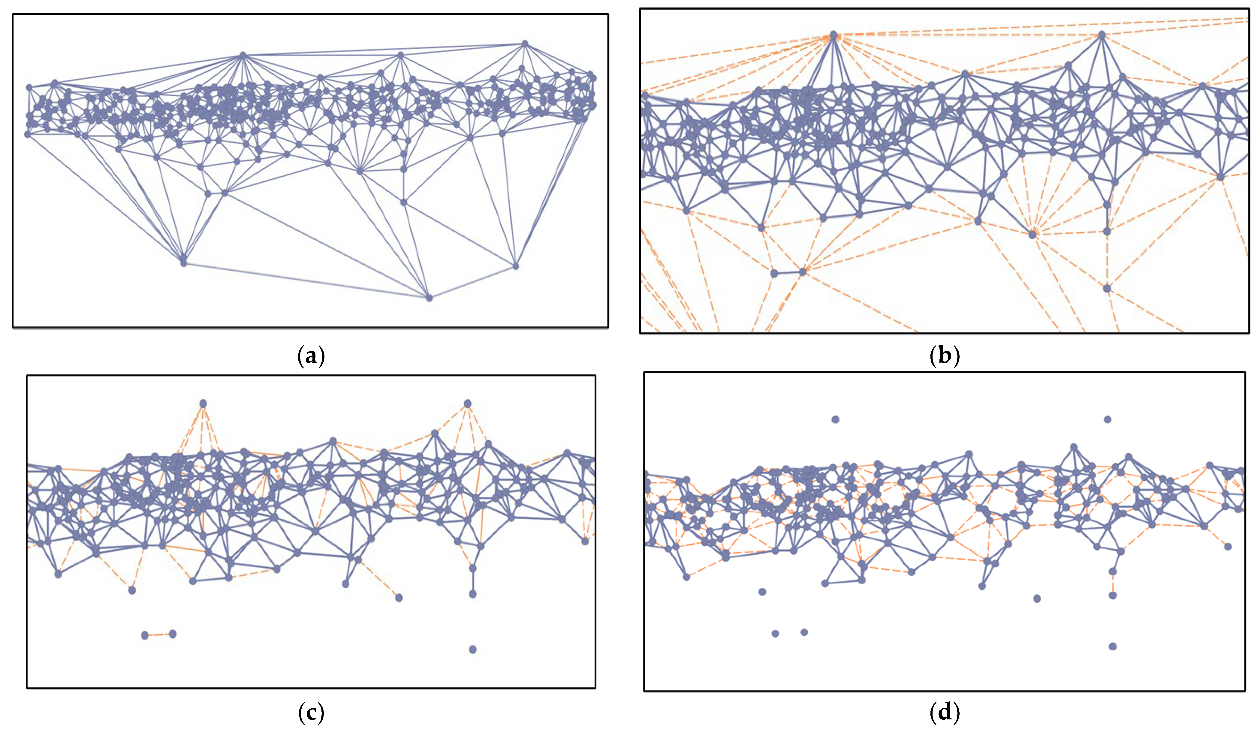
    • Construct the Delaunay triangulation DT of S (Figure 3a); the time complexity is O(NlogN).
    • For each point, calculate the G l o b a l _ M e a n   D T and Global _ Variation   D T in the Delaunay triangulation and L o c a l _ M e a n   P i . The time complexity is linear to N.
    • Remove G l o b a l _ L o n g _ E d g e s to separate global outliers (Figure 3b). The time complexity is O(N).
  • Step 2 Remove second-order long edges at a local level:
    • For each point, calculate 2 O r d e r _ M e a n   P i and M e a n _ V a r i a t i o n P i . The time complexity is linear to N.
    • Remove L o c a l _ L o n g _ E d g e s to separate local outliers (Figure 3c). The time complexity is O(N).
  • Step 3 Deal with necks and chains:
    • Remove L o c a l _ L i n k _ E d g e s and separate final outliers (Figure 3d). The time complexity is O(N).
Thus, the total complexity of the ASCDT algorithm is about O(NlogN).

3.2. Temporal Outlier Detection Phase: MP-Outlier Detection

During the temporal outlier detection phase, to enrich the input features, we first extract a 6-dimensional feature vector for each point, consisting of velocity, acceleration, course, turning angle, turning rate, and sinuosity. The TCN-AE model is then used to identify time correlations between the trajectory sequences and to remove MP-outliers by comparing the reconstruction loss of each trajectory point with a given outlier threshold. Specifically, we add the SE channel attention mechanism to enhance the feature extraction capability of the TCN.

3.2.1. Feature Extraction

To tackle Challenge 2 presented in Section 2, we enrich the feature space by extracting physically meaningful features from the raw data to help TCN learn the dependencies of the input sequences. Following the latest research [22], this paper selects six movement features.
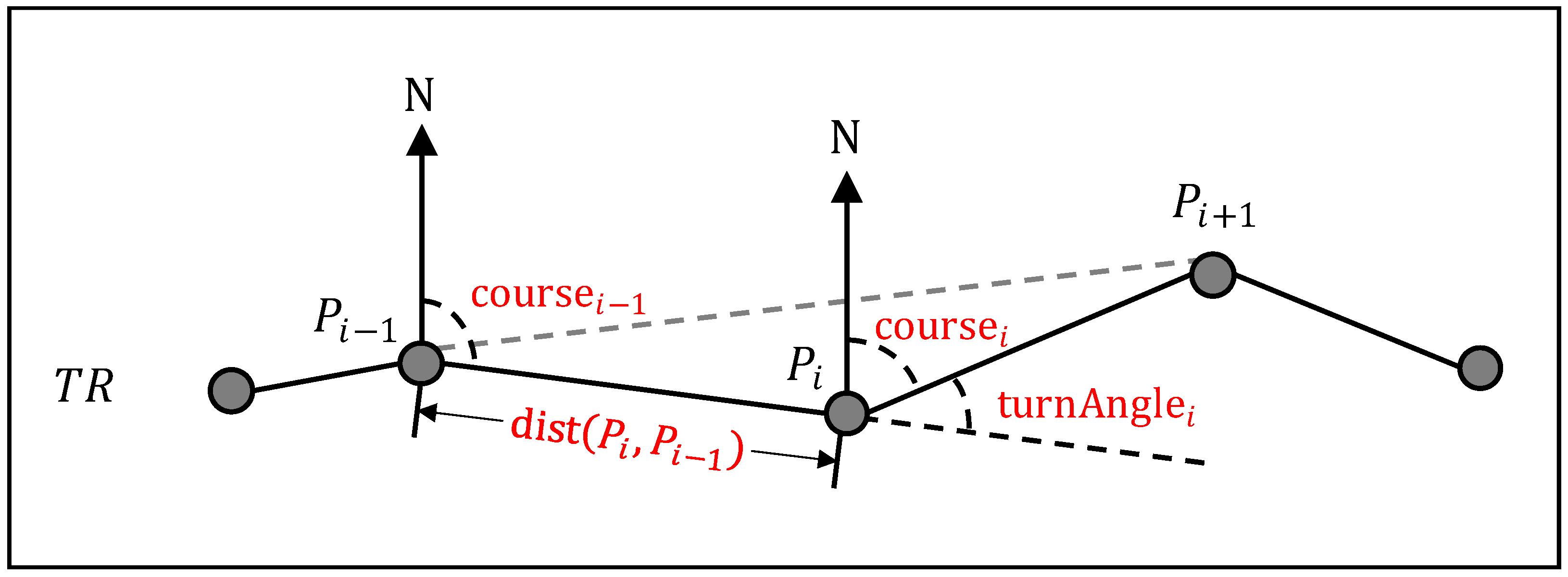
Given a trajectory T R = P 1 , P 2 , , P n , we extract a 6-dimensional feature vector for each point, consisting of velocity, acceleration, course, turning angle, turning rate, and sinuosity. As can be seen in Figure 4, each feature can be calculated as follows:
  • Velocity
The velocity is expressed as the ratio of the distance between two adjacent points to the time difference, indicating the target point movement rate. Outliers in a trajectory usually have greater velocity than their neighbors. For each point P i , the velocity can be represented as
v i = d i s t P i , P i 1 t i t i 1
where d i s t P i , P i 1 denotes the distance between point P i and its previous point P i 1 .
2.
Acceleration
The acceleration is expressed as the ratio of the velocity between two adjacent points to the time difference, indicating the rate of velocity change. Similar to velocity, outliers in a trajectory usually have a greater acceleration than their neighbors. For each point P i , the acceleration can be represented as
a i = v i v i 1 t i t i 1
3.
Course
The course is defined as the movement direction between consecutive points in a trajectory. It is expressed by taking the angle between the line connecting the current point with the latter point and the due north direction. Generally, if the course of a moving object changes suddenly, the point is more likely to be anomalous. For each point P i , the course can be represented as
c o u r s e i = a r c t a n x , y
x = c o s l a t i s i n l n g i l n g i 1
y = c o s l a t i 1 s i n l a t i s i n l a t i 1 c o s l a t i c o s l n g i l n g i 1
4.
Turning Angle
The turning angle represents the change between the heading of two adjacent points. Compared with the surrounding trajectory points, those points with significantly different turning angle are more likely to be outliers. For each point P i , the turning angle can be represented as
t u r n A n g l e i = c o u r s e i 1 c o u r s e i
5.
Turning Rate
The turning rate is expressed as the ratio of the turning angle between two adjacent points to the time difference, indicating the rate of turning angle change. For each point P i , the turning rate can be represented as
ω i = t u r n A n g l e i t u r n A n g l e i 1 t i t i 1
6.
Sinuosity
The sinuosity is defined as the ratio of the moving distance between three adjacent points to the distance of a straight line between two endpoints. Outliers in a trajectory usually have greater sinuosity than their neighbors. For each point P i , the sinuosity can be represented as
s i = d i s t P i 1 , P i + d i s t P i , P i + 1 d i s t P i 1 , P i + 1

3.2.2. MP-Outlier Detection with TCN-AE

To tackle Challenge 3 presented in Section 2, we are inspired by the TCN-AE model, since the outlier detection task of GPS trajectories is similar to time series, where trajectories can be treated as input sequences.
  • Temporal Convolutional Network (TCN)
The TCN was proposed in a recent study [23]. It consists of a 1D fully convolutional network (FCN), causal convolutions, dilated convolutions, and residual connections. FCN is mainly used to fulfil the principle that the output of all convolutional layers has the same length t, with zero padding to ensure subsequent layers that are the same length as previous layers.
Causal convolutions. Causal convolutions are used to ensure no information “leakage” from future to past. To ensure that, the output of each convolution layer at time step i corresponds only with the current layer and the previous layer, i.e., the output y i is predicted only utilizing current and past input X 1 : i for preventing future input X i + 1 : t leakage.
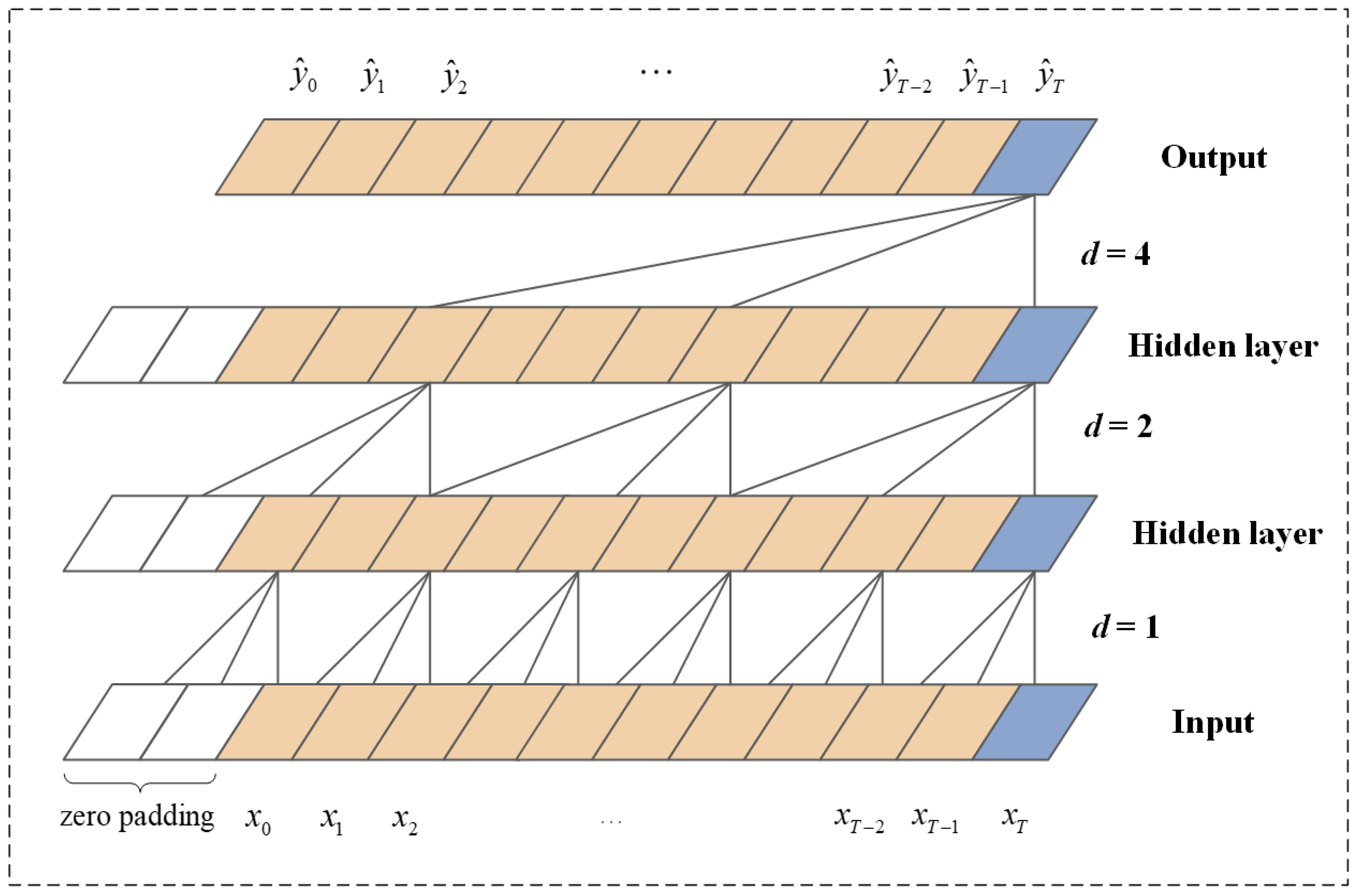
Dilated convolutions. With the time series containing long temporal dependencies, it is generally expected that the network will be able to retain long-term information. However, the sample causal convolutions are limited to the length of the receptive field unless the convolution layers are stacked in large numbers. It makes casual convolution challenging to apply to sequence tasks. To solve the problem of heavy calculation costs, dilated convolutions are employed to provide an exponentially large receptive field with limit layers. More specifically, for an input sequence X 1 : t = x 1 , x 2 , , x t and a filter f = 0 , 1 , , k 1 , the output of the dilated convolution operation F is defined as
F x i = X   d f x i = j = 0 k 1 f ( j ) · x i d · j
where * denotes the convolution operator, F x i is the output of the dilated convolution operation, and d is the dilation factor. When d = 1, the dilated convolutional layer reduces to a regular convolutional layer.
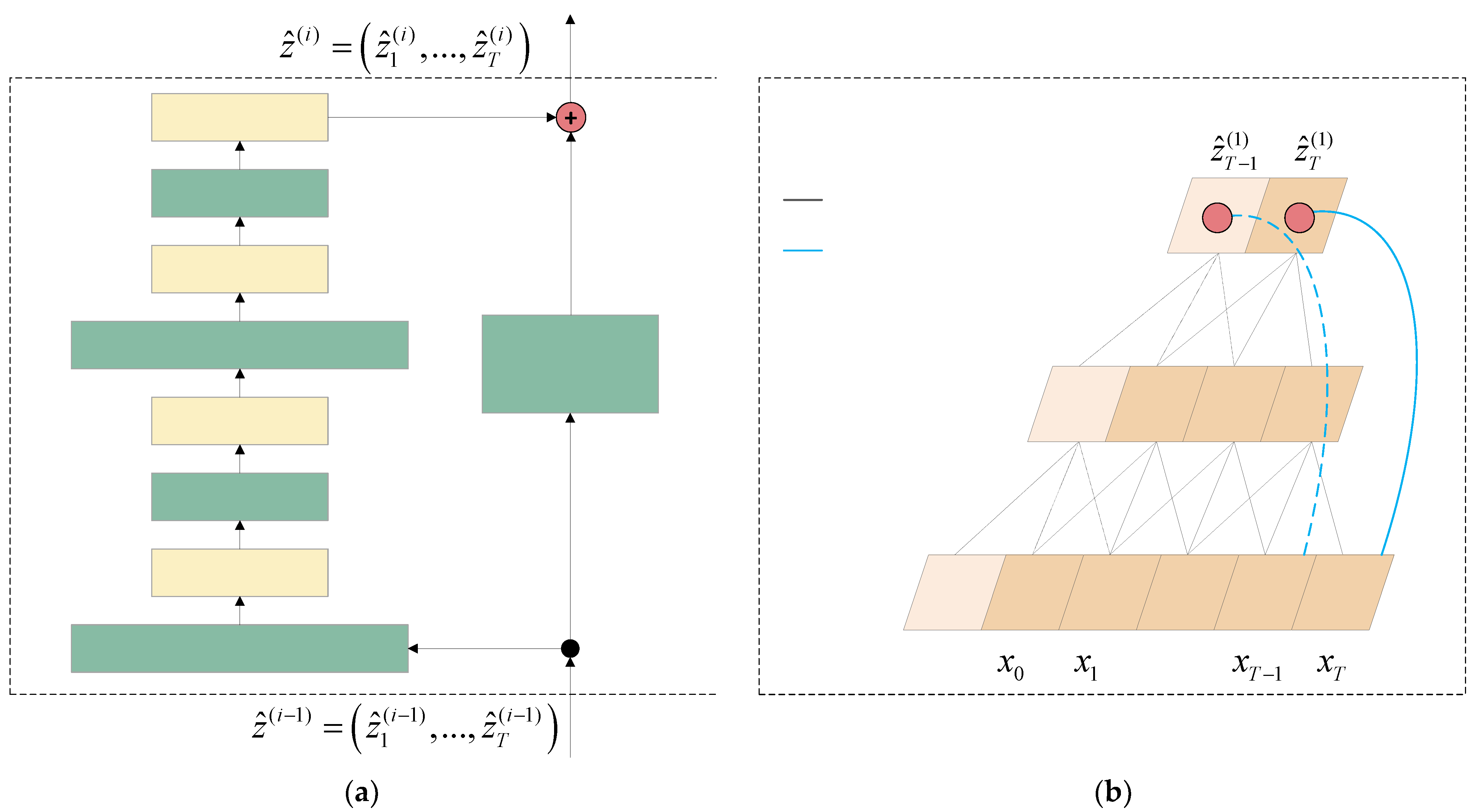
Figure 5 shows a dilated convolution schematic with dilated factors d = 1, 2, 4 and a filter size of k = 3. The acceptance area covers all the values of all the input sequences.
Residual connections. When causal convolutions and dilated convolutions are applied to the TCN, the network depth increases, which may result in gradient disappearance or gradient explosion. To solve this problem, residual connections are introduced to the network. Residual connections are used in ResNet, which are allowed to pass information in a cross-layer way. Many researchers have demonstrated that deep networks are in need of residual connections to prevent overfitting. A residual block contains two convolutional layers and a nonlinear mapping. In each layer, a weight regularization and a dropout algorithm are also added to regularize the network to prevent deep network overfitting. To reduce the dimensionality, an additional 1 × 1 convolution is also included, which makes the two tensors the same shape (Figure 6). The input x is weighted and fused into the output f(x) to produce the final output y:
y = A c t i v a t i o n x + f x
where A c t i v a t i o n ( ) is the activation function.
2.
SE Attentional Mechanism
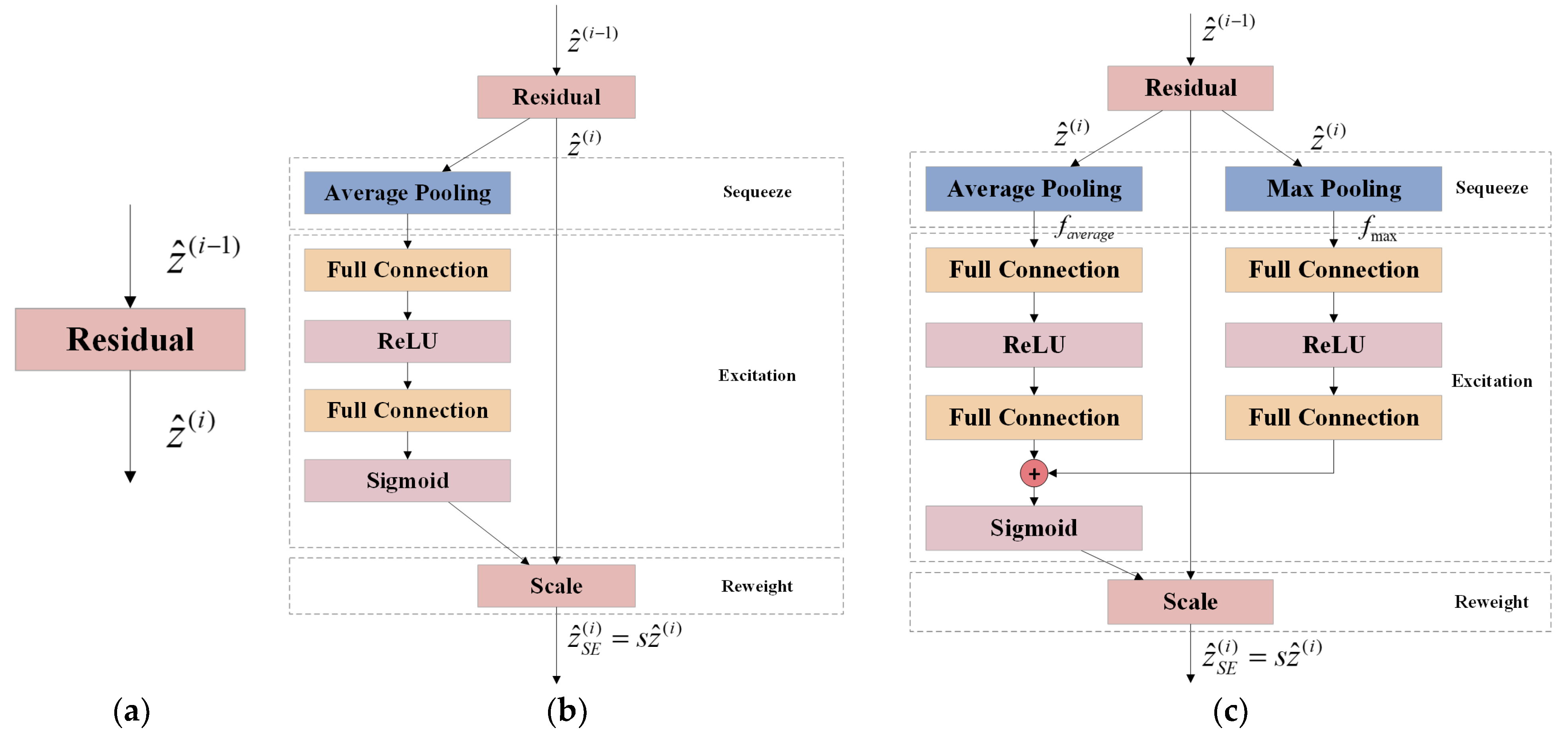
In the convolutional network, by default, each channel of the feature map is equally important, while in reality, the importance of different channels varies. To enhance the feature representation capability of the model, the channel attention mechanism in the SE block is introduced to improve the TCN. Essentially, the SE block assigns a weight to each channel of features so that the model focuses on those channels with key features and suppresses any channels with non-key features, improving the model’s ability to extract features. An SE block is composed of two operations: a squeeze function, which aggregates the global features of each feature map and extracts the most important information for each channel, and an excitation function, which calculates the dependencies between feature channels to obtain the importance weight coefficients of each channel.
As the attention mechanism for this residual block, the SE block is introduced after each layer of the TCN. The original SE block only uses global average pooling. To enhance the ability of the SE block to express global features, we add global maximum pooling to the original SE block. The SE-TCN residual block is shown in Figure 7.
The output after squeeze is obtained by
f average   = F s q 1 ( z ^ ( i ) ) = 1 H j = 1 H z ( j )
f m a x = F s q 2 z ˆ i = m a x z ˆ i
where z ˆ i 1 = z ˆ 0 i 1 , , z ˆ T i 1 and z ˆ i = z ˆ 0 i , , z ˆ T i are the input and output of the TCN residual block for the i-th residual block; f average and f max are the results of global average pooling and global maximum pooling for a single feature channel, respectively.
The output after excitation is obtained by
s = F e x f , W = σ g f , W = σ W average 2 δ W average 1 f average + W m a x 2 δ W m a x 1 f m a x
where W average 1 , W average 2 , W max 1 , W max 2 are the matrix parameters to be learned to calculate the correlation of features between channels; s is the weighting factor for the individual channel.
Finally, the channel weights of the above output are multiplied by the original features, thus realizing the redistribution of the original features in the channel dimension.
z ˆ S E i = F s c a l e z ˆ i , s = s z ˆ i
where z ˆ SE i = z ˆ S E 0 i , , z ˆ S E T i is the output of the i-th TCN residual block after weighting the weight coefficients by the SE block, i.e., the output of the SE-TCN residual block.
3.
Outlier Detection Model with TCN-AE
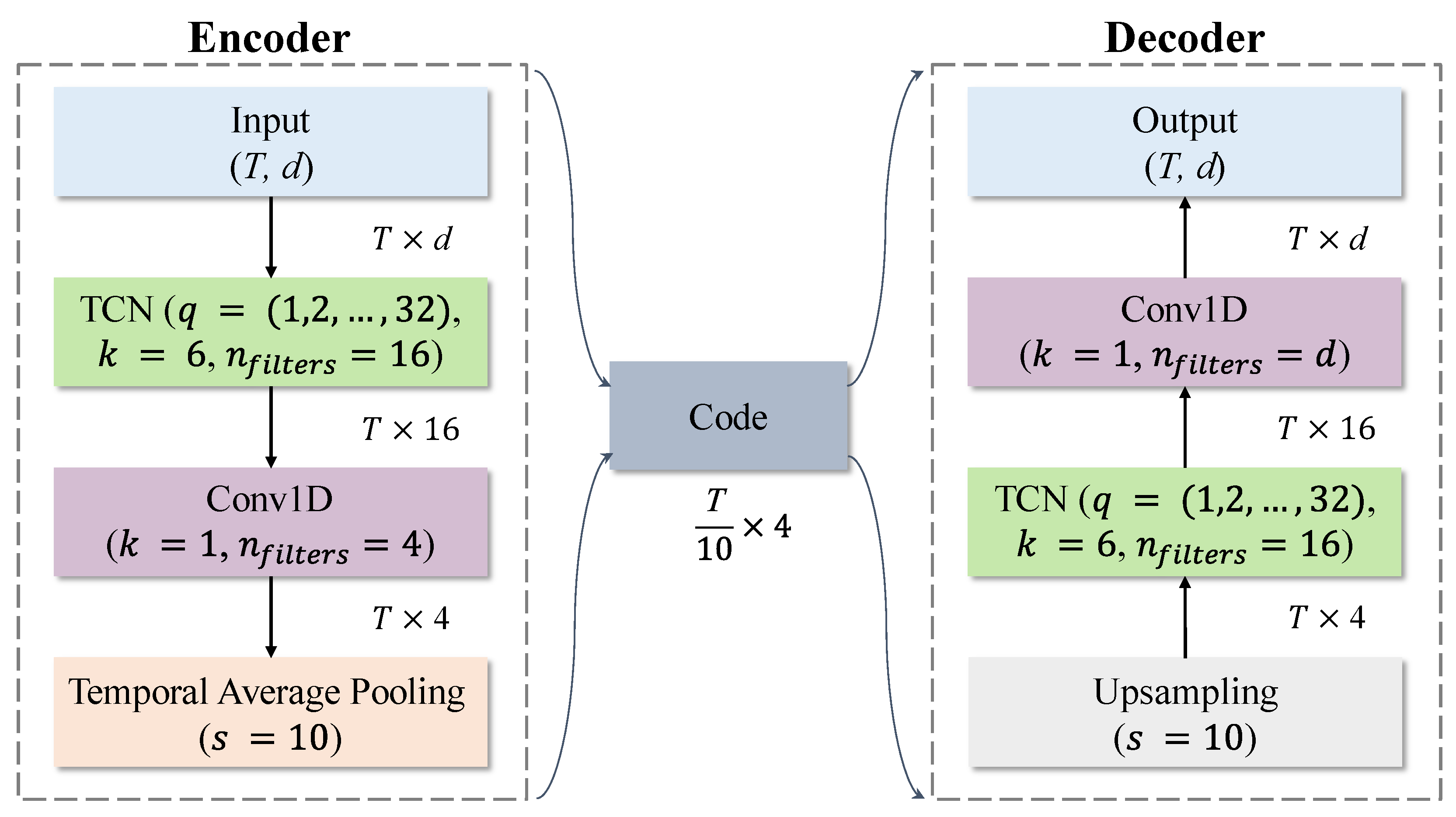
As illustrated in Figure 8, TCN-AE is designed to reconstruct the input sequence X = x 1 , x 2 , , x m T into an output sequence X ˆ = x ˆ 1 , x ˆ 2 , , x ˆ m T , which is composed of an encoder network and a decoder network. Essentially, the TCN-AE proposed here is similar to other autoencoder architectures. However, it differs from conventional autoencoders in that it combines causal and sparse convolutional layers instead of fully connected layers. Consequently, the network is more flexible for variable input sizes and more sensitive to temporal correlation. The central idea is to encode the input sequence compressively for creating a compact representation, which forces the network to learn the most representative patterns in the original input and to accurately reconstruct the original input. Conceptually, the TCN-AE learns to ignore data noise and trains the network for the purpose of minimizing the reconstruction loss of the input sequence. As a result, the anomalous data will have a larger reconstruction loss than normal data. Based on this, the TCN-AE can detect the anomalous data of GPS trajectories through its reconstruction loss.
Encoder. The encoder learns how to compress the original input sequence into a more compact representation that captures the main characteristics and considers the dependencies in sequential order. In the encoding phase, the encoder passes an input sequence through a TCN, a 1 × 1 convolutional layer and an average-pooling layer. As we mentioned before, for the encoder to generate the most significant features of an input sequence, it is required to analyze both short-term and long-term patterns. To tackle this challenge, the TCN is introduced to the encoder part. Then, the convolutional layer is used to reduce the dimension of the feature map, and the average-pooling layer is used to down-sample the time series by a specified factor.
Decoder. The decoder attempts to reconstruct the compact representation (the output of the encoder) into original input sequence. In the decoding phase, to restore the length of the original input sequence, we first use an upsample layer. Next, the upsampled sequence passes through a second TCN, which has the same structure as the encoder but with independent weights. Finally, the dimension of the original input sequence has to be restored. For this purpose, the decoder passes another 1 × 1 convolutional layer with filters that have the same number as the dimension.
After decoding, the network outputs a reconstruction error score for each trajectory point. Low scores indicate normal behavior, whereas high scores indicate abnormal behavior. By setting a threshold, each point is classified as nominal or outlier.

4. Experiment

4.1. Dataset

We validated the effectiveness of our model on a real-world vehicle trajectory dataset from the Beijing Taxi Administration Office. The dataset contains trajectories of 8422 drivers and 874,094 GPS records in the Haidian district, Beijing over a period of 24 h on 9 December 2018. All the trajectories are completed and sampled in 15~25 s. It covers a rectangular area from (39.8885, 116.0357) to (40.1545, 116.3879) around 30 km long and 29 km wide.
For the LO-outlier cleaning experiment, we randomly selected an area containing 10 roads and 19,887 GPS points as the evaluation data. After removing the offset points from the entire dataset, we split the remaining trajectory point dataset into training set, validation set, and test set with a splitting ratio of 6:2:2. The test set is labeled by multiple experiencers based on the position, velocity, and acceleration for each point in the trajectory. The outlier points are labeled as 1 (positive category), and normal points are labeled as 0 (negative category). All outlier detection algorithms are trained unsupervised. Actual outlier labels are only used at test time.

4.2. Evaluation Criteria

This paper uses Accuracy, Precision, Recall, and F1-score as the evaluation index [24]. The calculations are shown in Equations (25)–(28). With a higher Accuracy, Precision, Recall, and F1-score, the outlier detection method is more accurate.
  A c c u r a c y = T P + T N T P + F P + F N + T N
P r e c i s i o n = T P T P + F P
R e c a l l = T P T P + F N
F 1 s c o r e = 2 Precision Recall Precision + Recall
Outlier thresholds are set based on false negatives (Recall) and false positives (Accuracy). Thus, thresholds are determined based on equal accuracy (EAC), a performance metric which guarantees that accuracy and recall are approximately equal (the difference between accuracy and recall is less than 1%). Alternatively, the threshold can be applied to all the trajectory data by selecting the best threshold (F1-Score maximization) for a small portion of the trajectory data. For practical applications, this approach is more realistic because few labeled data are usually available.

4.3. Experiment Settings

The ASCDT algorithm is implemented using PySpark v3.3.1. As an LO-outlier, we set those points without any remaining edges. After removing offset points, the input to each algorithm is a 6-dimensional movement feature vector for each trajectory point.
We compared our unsupervised CTOD algorithm to other unsupervised outlier detection algorithms; each setting is as follows:
  • IF [25]: IF (scikit-learn, v0.23.2) uses a number of 1000 base estimators in the ensemble and a sliding window size of w = 50.
  • VAE [26]: LSTM-AE is implemented using the PyTorch framework. Both encoder and decoder use a single hidden layer with 400 dimensions, and the potential dimension is 200 dimensions.
  • LSTM-AE [27]: LSTM-AE is implemented using the PyTorch framework. The encoder uses a 2-layer LSTM network with 128 units in the first layer and 64 units in the second layer. The decoder is the reverse.
  • TCN-AE (baseline) [28]: Baseline TCN-AE is also implemented using the PyTorch framework. Both encoder and decoder use six dilated convolutional layers, respectively, and sixteen filters with a kernel size of k = 6.
  • CTOD: TCN-AE is implemented using the PyTorch framework. Both the encoder and decoder use six dilated convolutional layers, respectively, and sixteen filters with a kernel size of k = 6. The global maximum pooling and the global average pooling are both added in the SE residual block.

4.4. Experiment Results

4.4.1. Experiment 1: Location Offset Point Cleaning Effectiveness Evaluation

As an example, Figure 9 shows the effectiveness of the LO-outlier detection. In the case of Figure 9a, sporadic trajectory points outside of the road are well detected as offset points. As seen in Figure 9b, many trajectory points are collected in a parking area. They are not anomalous points, despite being outside the road.
The results of the cleaning effectiveness evaluation are shown in Table 1; 96.74% of the total trajectory points are correctly classified, and 87.47% of all the 3830 offset points are detected. This experiment verifies that the method can successfully remove the LO-outlier from the raw trajectory data without using map information.

4.4.2. Experiment 2: Extracted Outlier Points Evaluation

  • Overall Performance
The performance of different approaches for trajectory outlier detection is presented in Table 2. We observe that CTOD (F1-score = 0.8985) has the highest performance, followed by LSTM-AE (F1-score = 0.8806), baseline TCN-AE (F1-score = 0.8557), and VAE (F1-score = 0.8491), while IF performs the worst (F1-score = 0.7289). Moreover, based on the nonparametric Wilcoxon signed-rank test [29], we calculated the p-values to assess the significance of the results. The null hypothesis of the Wilcoxon test is that the F1-score of CTOD is smaller than the comparison algorithm. The table shows the p-values used to compare the F1-score of each algorithm with CTOD. The performance of CTOD is significantly higher than that of the other algorithms (p < 0.05, rejecting the null hypothesis at the 5% confidence level).
2.
Impact of Different Outlier Thresholds
We investigated the relationship between the reconstruction loss threshold and the outlier detection results. The effectiveness of the CTOD algorithm varies for different thresholds. As seen in Table 3, the detection metric F1-score reached a peak of 89.85% at a threshold value of 0.003.
Moreover, we also investigated the impact of threshold selection on detection results when only a small proportion of the trajectory dataset is used. Our experiment selected 10% of the dataset, and we determined the threshold for maximizing the F1-score on this subset. Taking into account the randomness of the results that resulted from the selection of different sub-data sets, we repeated the whole process ten times and averaged the results. We adjusted the threshold for 10% of the dataset, and then we evaluated the remaining 90%. As seen in comparison to Table 4, the F1-score of the algorithm deteriorates, but results are similar. Therefore, we can conclude that the method of selecting the best threshold from the subset is valid and will work in real-world situations.
3.
Impact of Reconstruction Loss Functions
The purpose of this experiment is to understand the sensitivity of different reconstruction loss functions on detection accuracy. Three reconstruction loss functions were investigated. They are root mean square error (RMSE), mean absolute error (MAE), and mean squared error (MSE), respectively. The definitions of these functions are described in the following equations.
R M S E = i = 1 n x i x ^ i 2 n
M A E = i = 1 n | x i x ^ 1 | n
M S E = i = 1 n ( x i x ^ i ) 2 n
where n represents the total number of samples, x i is the original input sample, and x ˆ i is the output.
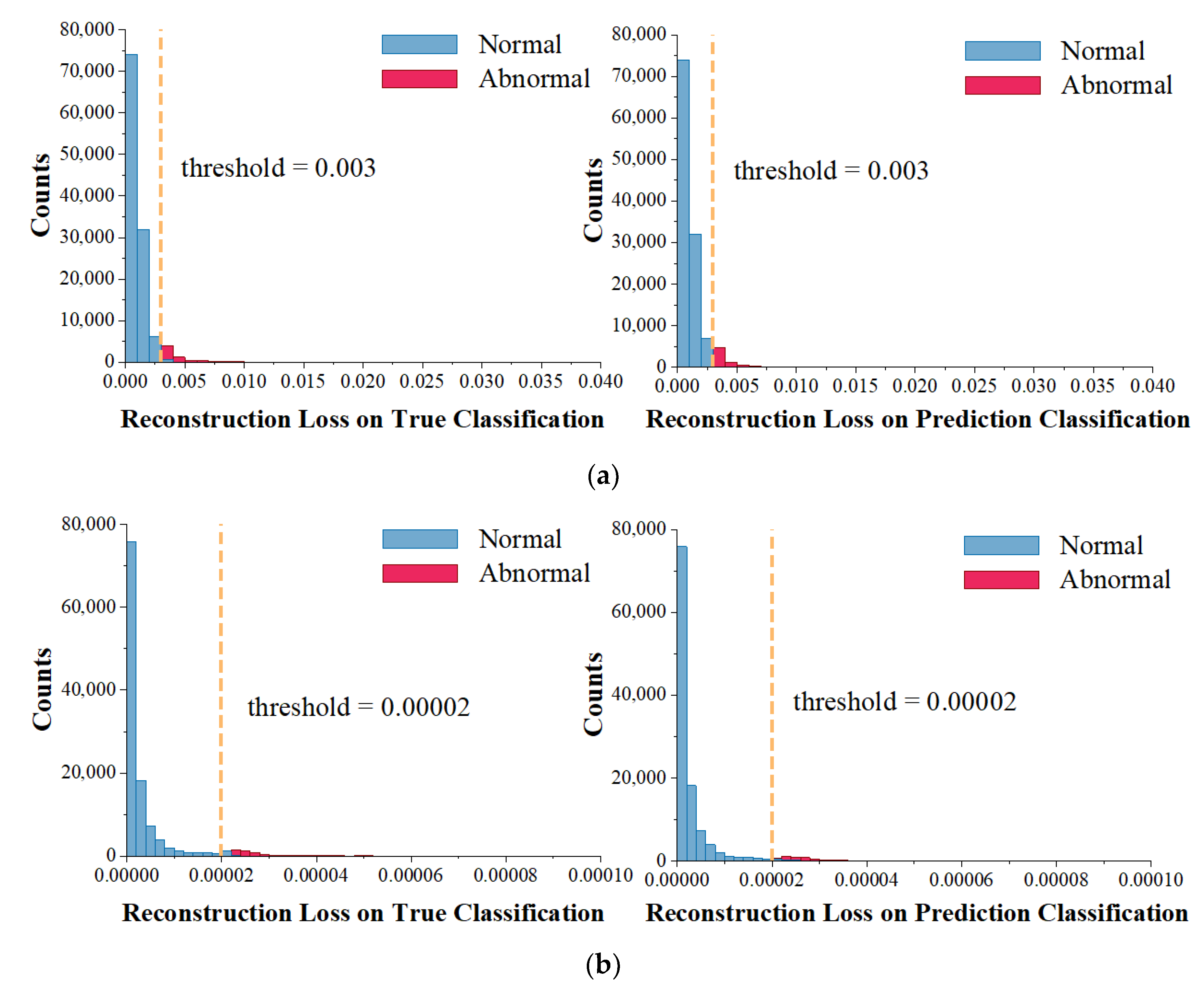
Figure 10 illustrates the relationship between reconstruction loss values and threshold values. We can clearly see that most of the trajectory points have a reconstruction loss below the threshold, and these points are marked as normal. In contrast, those trajectory points marked as abnormal have a greater reconstruction loss than the threshold. The reconstruction loss values of the real classification and predicted classification are highly consistent with their reconstruction loss distribution ranges.
As seen in Table 5, based on the three loss functions used, we obtained different thresholds. In spite of this, there are few differences between the evaluation results of the three loss functions. Among them, MAE provides the best detection results, while RMSE and MSE have essentially the same detection results.

5. Conclusions

Crowdsourcing trajectory data contains a large amount of information relevant to daily life, and it has great research potential. For example, the living habits of the residents of a city can be obtained by mining their trajectories, which in turn gives a deeper understanding of the culture and economy of the city. Meanwhile, information about popular locations and road conditions can be gathered from the trajectories in a city, and this information offers corresponding references to the control and administration of traffic and tourism events. Moreover, correlation analysis of trajectory data with other social, economic, and demographic data can reveal the flow pattern of the urban population, social activity dynamics, energy consumption distribution, and environmental pollution status, which can enhance urban management decisions. Due to various reasons such as technical limitations, there is inevitably a large amount of noise in the existing trajectory data, so the quality assurance of the trajectory data does the necessary groundwork for reliable research results.
In this paper, we proposed a crowdsourcing trajectory outlier detection framework called CTOD. The framework contains two phases. First, based on the ASCDT algorithm, LO-outliers are removed by calculating the local density adaptively and constraining the edge length of the triangulation. Second, based on the TCN-AE, MP-outliers are removed by mining the trajectories for internal temporal correlation features. The feature extraction and attention mechanism are implemented to improve performance. Our study result shows that it can effectively detect trajectory outliers. In general, our method has a F1-score about 2% higher than the LSTM-AE, about 5% higher than the VAE, and about 15% higher than the IF. Overall, the enhanced TCN-AE architecture is more advantageous for trajectory sequences. There are several more advantageous properties of the improved TCN-AE architecture for time series that might contribute to this:
  • Acceptance field: With the dilated convolutional structure, the acceptance field can easily be scaled down to the required size, allowing it to capture long-term time dependences more effectively.
  • Skip connection: With skip connection, TCN-AE is less sensitive to the choice of dilated factors. For example, we can select the dilated factors q = 1 , 2 , , 32 or q = 1 , 2 , , 64 , with similar results.
  • Hidden representations: By exploiting the output of the intermediate dilated convolutional layers, the input features can be accurately reconstructed at different timescales.
  • Number of weights: TCN-AE requires fewer trainable weights than other architectures, such as recurrent neural networks.
  • SE attention mechanism: With the SE attention mechanism, different contribution levels can be assigned to the constructed 6-dimensional input features, resulting in a more effective feature compression.
  • In this paper, the threshold for outlier detection is obtained through continuous experimental testing. Our threshold produces good outlier detection results. In future work, we intend to explore trajectory outlier detection algorithms by setting sensitive parameters automatically.

Author Contributions

Conceptualization, X.Z. and C.X.; methodology, X.Z.; validation, X.Z. and C.X.; data curation, D.Y.; writing—original draft preparation, X.Z.; writing—review and editing, X.Z., C.X. and Z.W.; visualization, X.Z.; supervision, D.Y.; project administration, D.Y.; funding acquisition, D.Y. All authors have read and agreed to the published version of the manuscript.

Funding

This research was funded by the Jilin Special Fund for Industrial Innovation, grant number 2019C024 and the Jilin Science and Technology Development Project was funded by 20190101023JH.

Institutional Review Board Statement

Not applicable.

Informed Consent Statement

Not applicable.

Data Availability Statement

Not applicable.

Acknowledgments

The authors also thank the associate editor and the reviewers for their useful feedback that improved this paper.

Conflicts of Interest

The authors declare no conflict of interest.

References

  1. Yuan, G.; Sun, P.; Zhao, J.; Li, D.; Wang, C. A Review of Moving Object Trajectory Clustering Algorithms. Artif. Intell. Rev. 2017, 47, 123–144. [Google Scholar] [CrossRef]
  2. Xiao, P.; Ang, M.; Jiawei, Z.; Lei, W. Approximate Similarity Measurements on Multi-Attributes Trajectories Data. IEEE Access 2019, 7, 10905–10915. [Google Scholar] [CrossRef]
  3. Wang, C.; Ma, L.; Li, R.; Durrani, T.S.; Zhang, H. Exploring Trajectory Prediction Through Machine Learning Methods. IEEE Access 2019, 7, 101441–101452. [Google Scholar] [CrossRef]
  4. Kim, J.; Mahmassani, H.S. Spatial and Temporal Characterization of Travel Patterns in a Traffic Network Using Vehicle Trajectories. Transp. Res. Procedia 2015, 9, 164–184. [Google Scholar] [CrossRef] [Green Version]
  5. Meng, F.; Yuan, G.; Lv, S.; Wang, Z.; Xia, S. An Overview on Trajectory Outlier Detection. Artif. Intell. Rev. 2019, 52, 2437–2456. [Google Scholar] [CrossRef]
  6. Guo, T.; Iwamura, K.; Koga, M. Towards High Accuracy Road Maps Generation from Massive GPS Traces Data. In Proceedings of the 2007 IEEE International Geoscience and Remote Sensing Symposium, Barcelona, Spain, 23–28 July 2007; pp. 667–670. [Google Scholar]
  7. Cao, K.; Shi, L.; Wang, G.; Han, D.; Bai, M. Density-Based Local Outlier Detection on Uncertain Data. In Web-Age Information Management; Li, F., Li, G., Hwang, S., Yao, B., Zhang, Z., Eds.; Lecture Notes in Computer Science; Springer International Publishing: Cham, Switzerland, 2014; Volume 8485, pp. 67–71. ISBN 978-3-319-08009-3. [Google Scholar]
  8. Liu, Z.; Pi, D.; Jiang, J. Density-Based Trajectory Outlier Detection Algorithm. J. Syst. Eng. Electron. 2013, 24, 335–340. [Google Scholar] [CrossRef]
  9. Wang, J.; Rui, X.; Song, X.; Tan, X.; Wang, C.; Raghavan, V. A Novel Approach for Generating Routable Road Maps from Vehicle GPS Traces. Int. J. Geogr. Inf. Sci. 2015, 29, 69–91. [Google Scholar] [CrossRef]
  10. Yang, X.; Tang, L. Crowdsourcing Big Trace Data Filtering: A Partition-and-filter model. Int. Arch. Photogramm. Remote Sens. Spat. Inf. Sci. 2016, XLI-B2, 257–262. [Google Scholar] [CrossRef] [Green Version]
  11. Choi, M.-K.; Lee, H.-G.; Lee, S.-C. Weighted SVM with Classification Uncertainty for Small Training Samples. In Proceedings of the 2016 IEEE International Conference on Image Processing (ICIP), Phoenix, AZ, USA, 25–28 September 2016; pp. 4438–4442. [Google Scholar]
  12. Xu, S.; Zhu, J.; Shui, P.; Xia, X. Floating Small Target Detection in Sea Clutter by One-Class SVM Based on Three Detection Features. In Proceedings of the 2019 International Applied Computational Electromagnetics Society Symposium-China (ACES), Nanjing, China, 8–11 August 2019; pp. 1–2. [Google Scholar]
  13. Degirmenci, A.; Karal, O. Robust Incremental Outlier Detection Approach Based on a New Metric in Data Streams. IEEE Access 2021, 9, 160347–160360. [Google Scholar] [CrossRef]
  14. Liu, B.; Yanshan, X.; Yu, P.S.; Zhifeng, H.; Longbing, C. An Efficient Approach for Outlier Detection with Imperfect Data Labels. IEEE Trans. Knowl. Data Eng. 2014, 26, 1602–1616. [Google Scholar] [CrossRef]
  15. Bhatti, M.A.; Riaz, R.; Rizvi, S.S.; Shokat, S.; Riaz, F.; Kwon, S.J. Outlier Detection in Indoor Localization and Internet of Things (IoT) Using Machine Learning. J. Commun. Netw. 2020, 22, 236–243. [Google Scholar] [CrossRef]
  16. Abdallah, M.; An Le Khac, N.; Jahromi, H.; Delia Jurcut, A. A Hybrid CNN-LSTM Based Approach for Anomaly Detection Systems in SDNs. In Proceedings of the The 16th International Conference on Availability, Reliability and Security, Vienna, Austria, 17 August 2021; pp. 1–7. [Google Scholar]
  17. Canizo, M.; Triguero, I.; Conde, A.; Onieva, E. Multi-Head CNN–RNN for Multi-Time Series Anomaly Detection: An Industrial Case Study. Neurocomputing 2019, 363, 246–260. [Google Scholar] [CrossRef]
  18. Yang, D.; Hwang, M. Unsupervised and Ensemble-Based Anomaly Detection Method for Network Security. In Proceedings of the 2022 14th International Conference on Knowledge and Smart Technology (KST), Chon buri, Thailand, 26 January 2022; pp. 75–79. [Google Scholar]
  19. Yao, R.; Liu, C.; Zhang, L.; Peng, P. Unsupervised Anomaly Detection Using Variational Auto-Encoder Based Feature Extraction. In Proceedings of the 2019 IEEE International Conference on Prognostics and Health Management (ICPHM), San Francisco, CA, USA, 17–20 June 2019; pp. 1–7. [Google Scholar]
  20. Provotar, O.I.; Linder, Y.M.; Veres, M.M. Unsupervised Anomaly Detection in Time Series Using LSTM-Based Autoencoders. In Proceedings of the 2019 IEEE International Conference on Advanced Trends in Information Theory (ATIT), Kyiv, Ukraine, 18–20 December 2019; pp. 513–517. [Google Scholar]
  21. Deng, M.; Liu, Q.; Cheng, T.; Shi, Y. An Adaptive Spatial Clustering Algorithm Based on Delaunay Triangulation. Comput. Environ. Urban Syst. 2011, 35, 320–332. [Google Scholar] [CrossRef]
  22. Zhaorong, H.A.; Tinglei, H.U.; Wenjuan, R.E.; Guangluan, X. Trajectory Outlier Detection Algorithm Based on Bi-LSTM Model. J. Radars 2019, 8, 36. [Google Scholar]
  23. Bai, S.; Kolter, J.Z.; Koltun, V. An Empirical Evaluation of Generic Convolutional and Recurrent Networks for Sequence Modeling. arXiv 2018, arXiv:1803.01271. [Google Scholar]
  24. Naser, M.Z.; Alavi, A.H. Error Metrics and Performance Fitness Indicators for Artificial Intelligence and Machine Learning in Engineering and Sciences. Archit. Struct. Constr. 2021, 1–19. [Google Scholar] [CrossRef]
  25. Liu, F.T.; Ting, K.M.; Zhou, Z.-H. Isolation Forest. In Proceedings of the 2008 Eighth IEEE International Conference on Data Mining, Pisa, Italy, 15–19 December 2008; pp. 413–422. [Google Scholar]
  26. Kingma, D.P.; Welling, M. Auto-Encoding Variational Bayes. arXiv 2022, arXiv:1312.6114. [Google Scholar]
  27. Jia, Y.; Zhou, C.; Motani, M. Spatio-Temporal Autoencoder for Feature Learning in Patient Data with Missing Observations. In Proceedings of the 2017 IEEE International Conference on Bioinformatics and Biomedicine (BIBM), Kansas City, MO, USA, 13–16 November 2017; pp. 886–890. [Google Scholar]
  28. Thill, M.; Konen, W.; Wang, H.; Bäck, T. Temporal Convolutional Autoencoder for Unsupervised Anomaly Detection in Time Series. Appl. Soft Comput. 2021, 112, 107751. [Google Scholar] [CrossRef]
  29. Wilcoxon, F. Individual Comparisons by Ranking Methods. In Breakthroughs in Statistics; Kotz, S., Johnson, N.L., Eds.; Springer Series in Statistics: New York, NY, USA, 1992; pp. 196–202. ISBN 978-0-387-94039-7. [Google Scholar]
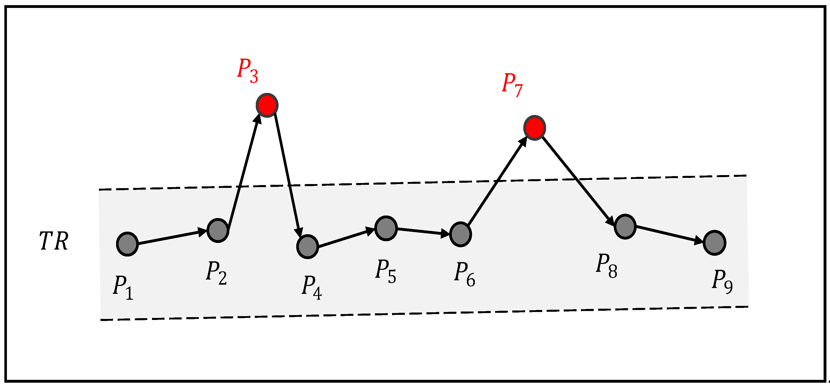
Figure 1. Example of Location Offset Point.
Mathematics 11 00620 g001
Figure 2. Framework of CTOD.
Mathematics 11 00620 g002
Figure 3. Schematic of ASCDT algorithm. (a) Delaunay triangulation; (b) global length constraint; (c) local length constraint; (d) local aggregation constraint.
Mathematics 11 00620 g003
Figure 4. A diagram of trajectory segment.
Mathematics 11 00620 g004
Figure 5. Schematic of TCN dilated causal convolution.
Mathematics 11 00620 g005
Figure 6. Schematic of TCN residual block. (a) a TCN residual block; (b) an example of a residual connection in TCN.
Mathematics 11 00620 g006
Figure 7. The comparison of TCN residual block and SE-TCN residual block. (a) TCN residual block; (b) SE-TCN residual block with average pooling; (c) SE-TCN residual block with average pooling and max pooling.
Mathematics 11 00620 g007
Figure 8. Our proposed TCN-AE model.
Mathematics 11 00620 g008
Figure 9. Example of location offset point detection. (a) example of well detected offset points. (b) example of trajectory points in a parking area.
Mathematics 11 00620 g009
Figure 10. Reconstruction loss distribution. (a) Reconstruction loss distribution based on MAE; (b) reconstruction loss distribution based on MSE; (c) reconstruction loss distribution based on RMSE.
Mathematics 11 00620 g010aMathematics 11 00620 g010b
Table 1. Cleaning effectiveness evaluation.
Accuracy (%)Precision (%)Recall (%)F1-Score (%)
96.7487.4792.1189.73
Table 2. Overall performance comparison.
AlgorithmAccuracy (%)Precision (%)Recall (%)F1-Score (%)p
IF97.0579.6167.2272.899.26 × 10-6
VAE98.2687.2482.7084.919.26 × 10-6
LSTM-AE98.5686.1390.0888.069.26 × 10-6
TCN-AE (baseline)98.3186.1285.0385.579.26 × 10-6
CTOD98.7989.4090.3189.85-
Table 3. Performance with different outlier thresholds.
No.ThresholdAccuracy (%)Precision (%)Recall (%)F1-Score (%)
10.00167.5915.4099.8626.69
20.00294.2350.6099.8667.17
30.00398.7989.4090.3189.85
40.003298.2792.8976.6684.00
50.003497.5995.5762.1475.31
60.003696.9497.2149.6765.75
70.003896.4597.9940.6757.48
80.00496.0798.1734.0550.56
90.00595.1398.5217.8930.28
100.00694.7197.8110.7019.28
110.00794.4696.596.3911.99
120.00894.3395.254.258.13
130.00994.2595.352.895.61
140.0194.1995.311.723.38
Table 4. Performance with outlier thresholds determine from only 10% of the outlier labels.
F1-ScoreAccuracy (%)Precision (%)Recall (%)F1-Score (%)
198.5683.9893.6388.54
298.6888.5188.7688.63
398.5283.6890.7987.09
498.4382.3592.7987.26
598.5784.2993.4688.64
698.7889.4990.1189.79
798.1378.2095.4185.95
898.4282.5493.4687.66
998.6788.2189.8889.04
1098.7388.9190.0289.46
Average98.5585.0291.8388.21
Table 5. Performance of different loss mechanisms.
MetricThresholdAccuracy (%)Precision (%)Recall (%)F1-Score (%)
RMSE0.0045098.5288.3886.2087.28
MAE0.0030098.7989.4090.3189.95
MSE0.0000298.5488.3686.6787.51
Disclaimer/Publisher’s Note: The statements, opinions and data contained in all publications are solely those of the individual author(s) and contributor(s) and not of MDPI and/or the editor(s). MDPI and/or the editor(s) disclaim responsibility for any injury to people or property resulting from any ideas, methods, instructions or products referred to in the content.