When Fairness Meets Consistency in AHP Pairwise Comparisons

Abstract

We propose introducing fairness constraints to one of the most famous multi-criteria decision-making methods, the analytic hierarchy process (AHP). We offer a solution that guarantees consistency while respecting legally binding fairness constraints in AHP pairwise comparison matrices. Through a synthetic experiment, we generate the comparison matrices of different sizes and ranges/levels of the initial parameters (i.e., consistency ratio and disparate impact). We optimize disparate impact for various combinations of these initial parameters and observed matrix sizes while respecting an acceptable level of consistency and minimizing deviations of pairwise comparison matrices (or their upper triangles) before and after the optimization. We use a metaheuristic genetic algorithm to set the dually motivating problem and operate a discrete optimization procedure (in connection with Saaty’s 9-point scale). The results confirm the initial hypothesis (with 99.5% validity concerning 2800 optimization runs) that achieving fair ranking while respecting consistency in AHP pairwise comparison matrices (when comparing alternatives regarding given criterium) is possible, thus meeting two challenging goals simultaneously. This research contributes to the initiatives directed toward unbiased decision-making, either automated or algorithm-assisted (which is the case covered by this research).

1. Introduction

The analytic hierarchy process (AHP) is a multi-criteria decision-making (MCDM) method developed by Saaty [1]. It is advantageous to solve many fundamental problems of selecting, ranking, and evaluating decision alternatives/options [2,3] when two or more criteria play a part in the decision. The method application covers topics in different areas, such as, for example, personal, engineering, social, and manufacturing [4]. Moreover, reviews of AHP applications are dedicated to specific fields, for example, construction [5], project management [6], operation management [7], medical and healthcare decision-making [8], and urban mobility [9].

AHP procedure includes mutually pairwise comparisons of both criteria and alternatives (according to the goal or each criterion separately) in pairwise comparison matrices (PCMs) using Saaty’s 9-point scale [10]. Despite the method’s vast application (AHP is the most used MCDM method according to Munier et al. [11]), a possibly large number of pairwise comparisons makes it challenging for decision-makers (DMs) to fill in PCMs with all required judgments. Therefore, logical inconsistency regarding pairwise comparison judgments is a leading methodological AHP-related research subject [12,13,14].

AHP is a specific quantitative MCDM method because it does not use direct weighting but compares each pair of criteria or alternatives [15]. DMs’ judgments are subjective and can lead to biased decisions, i.e., they can discriminate against some individuals or groups with specific sensitive properties in the final AHP-based ranking. This concern raises the issue of fairness, which is relatively new in MCDM (it motivates only a few papers from the field–e.g., [16,17,18,19]).

The limited human capacity to process data, today’s need for faster resolving complex situations, and the tendency to reduce subjective and biased human decisions motivate the use of artificial intelligence (AI) and machine learning (ML) algorithms. For example, fairness in hiring, lending, and imprisonment is related to AI decision-making applications [15]. Also, decision-making algorithms operate in complex socio-technical environments (for example, human-AI interactions make a significant part of risky decision-making in health and learning [20]). Human-AI interfaces will become increasingly widespread as ML algorithms are practical in real-world settings to help to improve human decision-making [21].

Although people feel more confident about being evaluated by algorithms when they perceive potential discrimination against them [22], algorithmic decision-making tends to produce unfair decisions implicitly and without real intention [23]. For example, socially-biased outcomes as a result of data-driven decision-making [24] or the so-called ”bias in, bias out“ can be because of trained algorithms on biased data [25]. Unintended discrimination is an intrinsic characteristic of AI [26]. Working with applicants’ databases is about statistical discrimination, especially regarding ML [15]. This study considers unintentional discrimination (unintentionally caused by biased DMs’ judgments in AHP pairwise comparisons) through a statistical measure called disparate impact (DI). We calculate it as a ratio of average ranking scores between two perceived groups of alternatives in the AHP-based ranking procedure–discriminated (i.e., disadvantaged) and privileged (i.e., advantaged) in achieving desirable ranking positions. Discrimination could happen even when data does not directly include sensitive attributes via highly predictive correlated criteria or the so-called ”proxies“ [23], which is often the case in MCDM (hence the term ”blindness to sensitive attributes“ in algorithmic decision-making [27]).

The main contribution of this paper is eliminating initial discrimination when it occurs in AHP pairwise comparisons while achieving a satisfactory consistency level (inconsistency score, i.e., consistency ratio–CR, lower than 0.1) or maintaining it at the already acceptable level. The paper’s experimental results confirm the following initial research hypothesis:

Hypothesis 1.

It is possible to computationally set AHP PCMs (when comparing alternatives regarding given criterium) to be both fair and consistent, with minimal correction of the initial comparison judgments fulfilled by human DMs.

In technical terms, the paper’s contribution is to set the discrete optimization problem (changing predefined initial values from Saaty’s 9-point scale positioned in the upper triangle–UT of AHP PCMs) and to solve a mathematical model (MM) with fairness and consistency nonlinear constraints. We use a metaheuristic population-based evolutionary optimization tool called a genetic algorithm (GA). It outperforms other nature-inspired algorithms on real-world discrete optimization problems, primarily in faster convergences and other performance indicators (along with the scatter search algorithm) [28].

The paper’s methodology contribution is also in offering an advanced procedure to efficiently improve consistency, starting from a consistent matrix, and by reducing the difficulty of combinatorial problems regarding searching feasible space while simultaneously does not harm fairness in the ranking of alternatives. The motivation is to solve logical consistency and to find room for fairness in the space of inconsistent and subjective DMs’ preferences.

Applying the proposed optimization procedure would provide approximately equable ranking outcomes to alternatives or in desired/legally defined proportion (observed by their group membership). The obtained research outcome (in its quality and framework) positions this research with other works intended against discrimination, such as in data mining [29], ML [30], AI ethics [31], and law [32], but with application in MCDM (which is quite a novelty, along with our unique methodological remarks).

The remainder of the paper contains several sections. The first part of the following section (Section 2) provides insight into related literature regarding the AHP method, the common-mentioned shortcomings of AHP pairwise comparisons, and fairness notes on AHP pairwise comparisons. A description of the research methodology takes part in the second part of the section. It includes the postulation of the discrete optimization toward desired consistent and fair AHP pairwise comparisons and the design of the synthetic experiment. Section 3 brings the results and proof of the research hypothesis. Discussion is in Section 4, while Section 5 concludes the research.

2. Materials and Methods

2.1. Insight into Related Literature

As the method for modeling complex problems in a hierarchical structure, AHP has motivated numerous articles in a growing trend:

• There are 35,430 articles published in the period 1980–2021 (from which 15,000 articles are from 2017–2021), according to Madzík and Falát [33] and based on Scopus;
• There are 8441 articles published in the period 1979–2017 (more specifically, there are 86 articles from 1979–1990, 716 articles from 1991–2001, and 7639 articles from 2002–2017), according to Emrouznejad and Marra [34] and based on ISI Web of Science;
• There are 9859 harvested articles published in the period 1982–2018, according to Yu et al. [35] and based on ISI Web of Science. This review also includes an improved Saaty’s version of the AHP, i.e., the analytic network process (ANP) that considers interaction and dependence among hierarchically structured elements.

Madzík and Falát [33] cluster nine AHP-related topics–i.e., Ecology and ecosystems, MCDM, Production and performance management, Sustainable development, Computer network, optimization & algorithms, Service quality, Fuzzy logic, Systematic evaluation, and Risk assessment. They also analyze the research impact of 26 subject areas of AHP applications (e.g., Engineering, Computer science, Environmental science, Business, management & accounting, Decision sciences, Mathematics, etc.) that contribute to the topics.

Reasons for the broader adoption of the method are in the following three principles described in [1], which contribute to the structured procedure of problem description and their well-grounded resolution:

• Up-down decomposition of decision problem in hierarchy levels, starting from the goal on the top, followed by criteria in the middle, sub-criteria if necessary, in the next/lower level(s), and finally, decision alternatives/options at the bottom of the elaborated hierarchy;
• Comparative judgments, i.e., comparisons of the decomposed elements from the same level in pairs (within PCMs) regarding the above-level goal or criteria (according to the nine-degree scale defined in [10]), to derive principal eigenvectors, i.e., relative priorities;
• Synthesis of the priorities, from local to the global plane, for overall alternatives’ ranking corresponding to the goal.

Despite these advantages, several shortcomings are also part of the discussion by a critic of the method. One of them is a rank reversal, which means that two alternatives (i.e., ranked items) could be reversed when one or more alternatives are added or deleted from the initially observed set of alternatives. To address this issue, Kong and Liu [36] developed an improvement that resolves the problem of alternatives’ discrepancies in the ordering caused by their dependencies. With similar motives, Lootsma [37] suggests additive AHP and multiplicative AHP that overcome the disadvantage of rank reversal in traditional AHP. Two variants of traditional AHP use different numerical scales to quantify preferential judgments in pairwise comparisons. The arithmetic scale in Additive AHP expresses DMs’ judgments via a difference in grades. Multiplicative AHP uses a scale with geometric progression to formulate DMs’ relative preferences. Maleki and Zahir [38] review 61 papers (from 1983–2011) with different causes of rank reversal.

Munier and Hontoria [39] state 30 subjects as a shortcoming of AHP: for example, regarding the presumption of independent criteria, concerns in pre-established quantifying preferences, questionable PCM fitting with many transitivity comparisons, AHP structure inadequate for modeling complex scenarios, etc.

2.1.1. Common-Mentioned Shortcomings of AHP Pairwise Comparisons

Let M be a PCM where $i=1,\cdots ,m$ specifies the number of items (criteria regarding the goal or alternatives regarding the observed criterion) we want to compare in pairs. The matrix M contains estimated comparisons:

$$M=\begin{array}{c}\hfill \left[\begin{array}{cccc}\hfill 1\hfill & i_{12}& \hfill \cdots \hfill & i_{1m}\\ \hfill i_{21}=\frac{1}{i_{12}}\hfill & 1& \hfill \cdots \hfill & i_{2m}\\ \hfill ⋮\hfill & ⋮& \hfill 1\hfill & ⋮\\ \hfill i_{m1}=\frac{1}{i_{1m}}\hfill & i_{m2}=\frac{1}{i_{2m}}& \hfill \cdots \hfill & 1\end{array}\right]\hfill \end{array}.$$

(1)

According to the goal or the observed criteria, the estimates based on Saaty’s 9-point scale tell us how much one item is more or less important than the other. Saaty’s scale (defined in [10]) includes discrete values from range 1 (equal importance) to 9 (extremely more important than) and their inverted values for the comparisons estimated with the less important clauses. The lower triangle of the matrix contains the inverted estimates from the UT, given the reciprocity of comparing items (e.g., $i_{m1}=\frac{1}{i_{1m}}$). Diagonals show the comparisons of two identical options, therefore, their equal importance.

Coordinates of the vector of weights, $w=(w_1,w_2,\cdots w_m)$, represent shares of preferences’ sums by rows in the total sum of all rows, as follows:

$$w_i=\frac{t_i}{{\sum }_i{t}_i},\sum _i{w}_i=1(i=1,\cdots ,m),$$

(2)

$$\begin{array}{cc}\left[\begin{array}{c}\hfill \begin{array}{cccc}\hfill 1\hfill & i_{12}& \hfill \cdots \hfill & i_{1m}\\ \hfill \frac{1}{i_{12}}\hfill & 1& \hfill \cdots \hfill & i_{2m}\\ \hfill ⋮\hfill & ⋮& \hfill 1\hfill & ⋮\\ \hfill \frac{1}{i_{1m}}\hfill & \frac{1}{i_{2m}}& \hfill \cdots \hfill & 1\end{array}\hfill \end{array}\right]& \begin{array}{c}\hfill t_1=1+i_{12}+\cdots +i_{1m}\hfill \\ \hfill t_2=\frac{1}{i_{12}}+1+\cdots +i_{2m}\hfill \\ \hfill ⋮\hfill \\ \hfill t_m=\frac{1}{i_{1m}}+\frac{1}{i_{2m}}+\cdots +1\hfill \end{array}& .\end{array}$$

The eigenvector method for checking the consistency of PCM includes defining a vector of eigenvalues $\lambda =({\lambda }_1,{\lambda }_2,\cdots {\lambda }_m)$, which coordinates we can calculate as follows (where $W={\left[w_i\right]}_{1\times m}$ is the one-dimensional matrix of the vector w):

$${\lambda }_i=\frac{ro{w}_i\left(M\right)\times W^T}{w_i},i=1,\cdots ,m.$$

(3)

The consistency index ($CI$) can be calculated according to the following formula (where ${\lambda }_i^{max}$ represents the maximum coordinate value in the vector $\lambda$, while m is the number of items) [10]:

$$CI=\frac{{\lambda }_i^{max}-m}{m-1}.$$

(4)

Consistency ratio ($CR$) represents the ratio of $CI$ and random consistency index ($RCI$) [40]:

$$CR=\frac{CI}{RCI}.$$

(5)

Table 1. $RCI$-values corresponding to the number of items/alternatives [1].

m	3	4	5	6	7	8	9	10
$\mathit{RCI}$	0.58	0.9	1.12	1.24	1.32	1.41	1.45	1.49

shows $RCI$-values corresponding to the observed number of items/alternatives (i.e., m), according to [1]. The values are experimentally obtained.

Only $CR$-values smaller than or equal to 0.1 (i.e., 10%) indicate an acceptable/tolerable consistency level [1], i.e., adequate compliance with the transitivity rule in the comparisons regarding the filled preference matrix M. For example, if an item, e.g., alternative $A_1$, is better than alternative $A_2$, and $A_2$ is better than $A_3$, then $A_3$ could not be better than $A_1$. In addition, it matters how many pairwise items are mutually better/worst compared to other possible combinations.

Analogously to the taxonomy of studies regarding the systematic review of an MCDM method (suggested by Mardani et al. [41]): utilized, integrated, proposed/applied, and modified or extended research, we search only for the last type in the context of the AHP method. We identify shortcomings of the traditional AHP method about common-mention issues in pairwise comparisons, organized in the following two streams, which motivated our research (others are also possible, for example, rank reversal issue):

• A possible large number of input judgments in the pairwise comparisons and logical inconsistency in PCMs (please see

  Table 2. An overview of AHP modifications dedicated to facilitating pairwise comparisons and improving logical consistency.

  Author(s)	Name	Purpose of Transformation	The Used Method	Field of Application
  Sangiorgio et al. [42]	Optimized-AHP (O-AHP)	It successfully overcomes the following drawbacks of classical AHP, common in situations when the number of criteria or alternatives is greater than nine: a large number of comparisons/judgments and the limited capacity of the human mind, consistency issue.	The weights evaluation procedure based on mathematical programming (MP) redefines the process of forming a judgment matrix in the following ways: It uses judgment ranges instead of the exact judgment assignments; An MP formulation provides the entries of the judgment matrix to minimize inconsistency.	Construction
  Ishizaka et al. [43]	AHPSort	It reduces the number of required comparisons and facilitates decision-making.	A new variant sorts alternatives into ordered predefined categories according to DMs’ preferences.	Supplier selection
  Ishizaka and López [44]	Cost-Benefit AHPSort	It provides better and easier comparisons and benchmarks for evaluating alternatives.	A modification of the AHPSort treats cost and benefit criteria separately, i.e., into two distinct hierarchies.	Performance analysis of offshore providers in the aerospace industry
  Li et al. [45]	Improved AHP (IAHP)	It improves consistency in PCMs when the number of elements equals five or more.	The improvement uses the sorting technique (instead of quantification on Saaty’s 9-point scale) to judge between two elements in pairwise comparisons.	Risk identification in construction
  Lin et al. [46]	Adaptive AHP approach ($A^3$)	It helps to improve consistency in pairwise comparisons, reduce costs and timeliness, and improve decision-making quality.	The approach uses a soft computing technique (i.e., a GA) to improve consistency automatically.	Construction
  Xiulin and Dawei [47]	Improved AHP	It overcomes the difficulties of making judgments according to the traditional nine-scaling method and blindness in checking consistency. It is helpful in the determination of target weights.	The improvement uses a 3-scale point method: 1/0.5/0 indicates that the $i^{th}$ alternative is more/equally/less important than the $j^{th}$ alternative.	Teacher evaluation
  Leal [48]	AHP-express	The simplified version helps make decisions in constrained times. It reduces the number of required comparisons and facilitates calculations.	The simplification requires only $n-1$ comparisons (n–number of alternatives) for each criterion, unlike $(n^2-n)/2$ required comparisons in traditional AHP.	Business application
  Chen [49]	Diversified AHP-tree approach	It allows diverse viewpoints of DMs regarding criteria relative importance.	The approach decomposes an inconsistent judgment matrix into several sub-judgment matrices. It uses the GA for solving nonlinear programming models to maximize the sum of distances between any two sub-judgment matrices.	Supplier selection
  Abastante et al. [50]	New parsimonious AHP methodology	It reduces the number of comparisons and inconsistencies and avoids rank reversal problems compared to the original AHP.	A newly developed proposal implies using reference objects for pairwise comparisons. It avoids comparisons of more relevant objects with less relevant ones.	General application

  for suggested modifications);
• Uncertain and subjective DMs’ judgments (please see

  Table 3. An overview of AHP modifications dedicated to overcoming uncertain and subjective DMs’ judgments.

  Author(s)	Name	Purpose of Transformation	The Used Method	Field of Application
  Nefeslioglu et al. [51]	Modified AHP (M-AHP)	It compensates for expert subjectivism in pairwise comparisons due to a lack of knowledge or data for the relevant problem.	A computer code is postulated on factors and the decision points, whereby the role of experts in preparing the comparison matrix is limited to defining the maximum scores for factors in the system.	Natural hazards
  Tesfamariam and Sadiq [52]	Fuzzy AHP (F-AHP)	It allows DMs to account for uncertainty (vagueness).	The fuzzy-based technique used fuzzy arithmetic operations. It aggregates the fuzzy global preference weights concerning each alternative.	Environmental risk management
  Banuelas and Antony [53]	Modified AHP (MAHP)	It includes uncertainty and managerial aspects (‘soft’ issues) in judgment comparisons and, therefore, a better understanding of the context of the applied technique.	The method incorporates uncertainty by using probabilistic distributions. It tests the results for statistical significance and analyses rank reversal using ANOVA.	Application in organizations
  Xu et al. [54]	Entropy weight modified AHP hierarchy model (EWMAHPHM)	It improves decision-making efficiency in changing environments where regional information is insufficient.	The method includes the entropy weight method in AHP. The construction of the distributed model precedes the entropy weight correction.	Information-based ecological environment construction
  Sadiq and Tesfamariam [55]	Intuitionistic fuzzy AHP (IF-AHP)	It handles both uncertainty categories–vagueness and ambiguity in human subjective evaluation.	The methodology uses intuitionistic fuzzy sets.	Environmental decision-making
  Lin et al. [56]	Improved AHP (IAHP)	It comprehensively determines the weights of risk indices.	The improvement uses the entropy weight method and integrates objective data variability with subjective judgments.	Flash flood risk assessment
  Deng et al. [57]	D-AHP	It provides a new, effective, and feasible expression of uncertain information.	The method extends the fuzzy preference relation approach by using the so-called D numbers, resulting from the Dempster–Shafer theory extension.	Supplier selection

  for modifications indicated).

2.1.2. Fairness Notes on AHP Pairwise Comparisons

As two sides of the same coin [58], bias and fairness appear differently. Mehrabi et al. [59] recognize 23 types of biases presented in data (directed to algorithms)–e.g., measurement bias; algorithms (directed to users)–e.g., algorithmic bias; and user experiences (directed to data)–e.g., historical bias. Different fairness definitions are also possible. Verma and Rubin [60] group them regarding statistical measures (as definitions based on predicted outcome–e.g., statistical parity as a measure of group fairness; predicted and actual outcomes–e.g., equal opportunity as false negative error rate balance; and predicted probabilities and actual outcome–e.g., calibration as a test-fairness measure) similarity-based measures (e.g., fairness through awareness), and causal reasoning (e.g., counterfactual fairness). Fairness definitions that include binary classifiers are concentrated on the confusion matrix [60] and have different perspectives (for DMs, applicants, and society) [61].

In MCDM, we can interpret fairness in different ways:

• Concerning DMs–it is applicable in group decision-making when decision systems should fairly include DMs’ opinions. For example, a decision support system for group MCDM can mitigate or eliminate biased DMs’ opinions [62] or follow a democratic approach in conflict situations by choosing a consensual value for parameter v (related to the VIKOR method, it equals 0.5) [63].
• Concerning decision criteria–criterion weights are essential for two levels of fairness: among criteria and alternatives [64]; while it is generally possible to introduce discrimination based on a single property (e.g., racial discrimination–[65], gender discrimination–[66], age discrimination–[67], etc.), several separate properties (i.e., multiple discrimination–[68]), or one joint property (i.e., intersectional discrimination–[69]). In MCDM, opposite to wash criteria about which alternatives are equally preferred [70], DMs can define criteria (or their weights) that favor/damage some alternatives or groups (the favored group is privileged, and the damaged group is unprivileged).
• Concerning the used algorithms–it can imply the absence of unintentional (coincidentally made) discrimination toward vulnerable groups in society that algorithmic decision-making techniques may amplify. The harmful practice is possible because of, for example, data that reflect historically widespread biases and contain the prejudices of prior DMs [71] or impose discriminatory inferences towards underrepresented groups [23].

We follow the identified pairwise comparison issues in this section with the idea that DMs can produce biased judgments that can lead to unfair decisions. Inconsistent and subjective judgments (for example, because of inadequate domain knowledge) weave a path for implicit bias. In this work, we cover unintentional discrimination defined via measure for group fairness, i.e., DI specified in Section 2.2.1, which arises from statistical parity fairness that suggests independence between sensitive attributes and decision outcomes [72]. We observe alternatives in PCMs about the given criterion and their belonging to the sensitive group.

2.2. Toward Consistent and Fair AHP Pairwise Methodology

Let A be PCM where $i=1,\cdots ,m$ specifies the number of alternatives (i.e., instances in a dataset) regarding criterion C. Matrix A contains estimates of two alternative comparisons:

$$A=\begin{array}{c}& \begin{array}{cccc}\hfill A_1\hfill & \hfill A_2\hfill & \cdots & \hfill A_m\hfill \end{array}\\ \begin{array}{c}\hfill A_1\hfill \\ \hfill A_2\hfill \\ \hfill ⋮\hfill \\ \hfill A_m\hfill \end{array}& \left[\begin{array}{cccc}\hfill 1\hfill & \hfill a_{12}\hfill & \hfill \cdots \hfill & \hfill a_{1m}\hfill \\ \hfill \frac{1}{a_{12}}\hfill & \hfill 1\hfill & \hfill \cdots \hfill & \hfill a_{2m}\hfill \\ \hfill ⋮\hfill & \hfill ⋮\hfill & \hfill 1\hfill & \hfill ⋮\hfill \\ \hfill \frac{1}{a_{1m}}\hfill & \hfill \frac{1}{a_{2m}}\hfill & \hfill \cdots \hfill & \hfill 1\hfill \end{array}\right]\end{array}.$$

(6)

An iterative weight determination method executes until the stabilization of the iterative vector, $w^{iter}=(w_1^{iter},w_2^{iter},\cdots w_m^{iter})$, for which the one-column matrix $W^{iter}={\left[w_i^{iter}\right]}_{m\times 1}$ can be calculated as follows: ${W^{iter}}^k=\frac{A\times {W^{iter}}^{k-1}}{{\sum }_{i}A\times {W^{iter}}^{k-1}}$. In other words, the process stops when ${W^{iter}}^{k-1}$ from the previous iteration (observed to a large number of decimals) is approximately equal to the current ${W^{iter}}^k$ (e.g., down below the predefined negligible threshold size):

$$\sum _{i=1}^m|{w_i^{iter}}^k-{w_i^{iter}}^{k-1}|<0.00001.$$

(7)

The eigenvector method for checking the consistency of PCMs includes defining a vector (one-dimensional matrix) of eigenvalues $\lambda$. Since ${W^{iter}}^{k-1}\approx {W^{iter}}^k$ in the last iteration (which corresponds to $W^{iter}$), $\lambda$ can be calculated as follows:

$$\lambda =\frac{A\times W^{iter}}{W^{iter}}.$$

(8)

2.2.1. Discrete Optimization Problem

Saaty’s 9-point scale for the pairwise comparisons [10] includes discrete values from range 1 (equal importance) to 9 (extremely more important than) and its inverted values for the unpreferred options. Therefore, we can define a dictionary with the following 17 keys/values in total:

$$\begin{array}{c}\hfill dict=\{1\to \frac{1}{9},2\to \frac{1}{8},3\to \frac{1}{7},4\to \frac{1}{6},5\to \frac{1}{5},6\to \frac{1}{4},7\to \frac{1}{3},8\to \frac{1}{2},\\ \hfill 9\to 1,10\to 2,11\to 3,12\to 4,13\to 5,14\to 6,15\to 7,16\to 8,17\to 9\}.\end{array}$$

(9)

The number of elements in the UT of matrix A equals $t=\frac{m\ast (m-1)}{2}$ and represents the number of unknowns (vector coordinates) we intend to solve. In their place come values from the dictionary, and they may repeat.

Based on the values of sensitive attribute s formally invisible in preference matrices, we can divide alternatives into two groups: discriminated ones (whereby $s=1$) and privileged ones (whereby $s=0$). Consequently, one-dimensional matrix $S={\left[s_i\right]}_{m\times 1}$, $i=1,\cdots ,m$, contains values $s_i\in \left\{0,1\right\}$ that correspond to each alternative/row in matrix A.

DI before optimization (${DI}_{bef}$) is the ratio of average AHP rank comparison scores before optimization (${\overline{R}}_{bef}$) between privileged and discriminated groups. Since the favored alternatives occupy higher rank positions and have a lower average rank score, ${DI}_{bef}$ takes the inverted value and should be equal to or greater than 0.8 (according to the “80% rule“ [73]) as follows [16]:

$${DI}_{bef}=1/\frac{{\overline{R}}_{bef[s=1]}}{{\overline{R}}_{bef[s=0]}}=\frac{{\overline{R}}_{bef[s=0]}}{{\overline{R}}_{bef[s=1]}}\ge 0.8.$$

(10)

If this group fairness condition is not satisfied, our method suggests recalculating ranks by changing initial preference estimations while considering consistency.

Our discrete optimization repairs initial $C{R}_{bef}$- and $D{I}_{bef}$-values to the desired level (after optimization), relying on the initial research hypothesis. The goal is a minimal correction of initial preferences in AHP PCMs, i.e., in their UTs before and after optimization (represented as absolute differences of the following vectors/one-column matrices: $|{U{T}_{bef}}_{t\times 1}-{U{T}_{aft}}_{t\times 1}|$). Consequently, the goal function ($f_d$) is the minimization of the sum of these differences from the first position to the last one:

$$\left(min\right)f_d=\sum _t\left|{{UT}_{bef}}_t-{{UT}_{aft}}_t\right|.$$

(11)

The MM for this optimization also includes two types of constraints. The first type is related to the consistency requirement, and the second type implies additional requirements, i.e., fairness constraints.

The consistency requirement hints at a value $CR\le 0.1$. There is no restriction on dictionary movement for PCM sizes less than or equal to 6 (experience has shown that the optimization successfully overcomes all set constraints for smaller matrices of magnitude, i.e., $m=4,5,6$). Any value from the dictionary can come to any t place in the UT. The only (conditionally speaking) restriction is that the total magnitude of changes in the original and new values vectors, which come to the UT positions, is minimal (regulated by $f_d$).

If the matrix size is larger than 6, the number of possible combinations to fulfill the UT positions is very high. For example, the number of possible combinations for a matrix size of 10 would be ${17}^{\frac{10\ast (10-1)}{2}}={17}^{45}$. To alleviate the combinatorial problem, we restrict the dictionary movement by three degrees of freedom for each position in the UT. In particular, we allow movement by three consecutive places to the left and the right of the initial key (i.e., the corresponding values defined in the dictionary). So, we narrow the search space to 7 combinations for each place in the UT.

To further facilitate the optimization task, our starting point is from a consistent matrix ($A_c$), calculated according to the following formula:

$$A_c=W^{iter}\times {({W^{iter}}^{-1})}^T.$$

(12)

The starting point is a consequence of the following theorem:

Theorem 1.

The space of admissible solutions (simultaneously consistent and fair matrix we are looking for) is not empty.

To support this claim, we adduce the following proof:

Proof of Theorem 1.

The unit square matrix is perfectly consistent ($CR=0$) and fair (all ranks equal to 1). □

Therefore, one solution is guaranteed, and the difficulty of the optimization problem lies in finding such a matrix that also has a small value of the objective function.

In the further procedure, we observe the UT of a consistent matrix $A_c$, i.e., its initial values. The idea is to find a close standardized value from a predefined scale for each initial value (i.e., before optimization). That is why we follow the idea of the symmetrical dictionary as follows:

$$\begin{array}{c}\hfill dic{t}_s=\{-8\to \frac{1}{9},-7\to \frac{1}{8},\cdots ,-1\to \frac{1}{2},0\to 1,1\to 2,\cdots ,7\to 8,8\to 9\}.\end{array}$$

(13)

We invert negative preferences (those less than 1) in the UT (e.g., $\frac{1}{\frac{1}{5}}=5$). Following, we round the latest values in the UT (e.g., $5\cong 5$) and subtract 1 (e.g., $5-1=4$). Where there were negative preferences, we multiplied the newly obtained values by $-1$ (e.g., $-1\ast 4=-4$). Please note that the key -4 corresponds to the initial value $\frac{1}{5}$ in $dic{t}_s$. We should increase each key from $dic{t}_s$ by 9 to conform to keys from $dict$ (e.g., $-4\to \frac{1}{5}$ from $dic{t}_s$ corresponds to $5\to \frac{1}{5}$ from $dict$). We have limited the movement through $dict$ by three places left and right concerning the initial position of the key (different degree of freedom is also possible) to reduce the number of possible combinations sufficiently. For limit keys, if it is not possible to move for three positions, we take the value of the minimum or maximum key, i.e., their corresponding values. For example, for key 2 in $dict$, you can only go one position to the left, or for key 15, you can only go two positions to the right.

The MM with $f_d$ objective function should meet the following fairness constraint (i.e., the lower limit):

$${DI}_{aft}=\frac{{\overline{R}}_{aft[s=0]}}{{\overline{R}}_{aft[s=1]}}\ge 0.8.$$

(14)

In addition to the lower limit, we introduce an upper limit (defined as in [16]):

$${DI}_{aft}\le \frac{1}{0.8}=1.25.$$

(15)

The upper limit is symmetric to the lower limit. Its purpose is to prevent the opposite effect, i.e., to harm the initially privileged group by reranking.

To solve this optimization with non-linear constraints, we use the GA as a population-based metaheuristic [74,75] used in operation management (OM) decision areas such as operations planning and control, process and product design, and operations improvement [76]. Besides OM issues, GA is also efficient in NP-hard problems in multimedia and wireless networking [74]. As an evolutionary computation algorithm that imitates the biological evolution process, it is suitable for soft computing in engineering challenges [77].

In addition to the previously explained goal function (Equation (11)), we define the following penalty functions for constraints (the first is related to consistency, and the second and third to fairness constraints):

$$\begin{array}{c}\hfill pen1=\left\{\begin{array}{cc}0,\hfill & \mathrm{for}{CR}_{aft}\le 0.1\hfill \\ \infty ,\hfill & \mathrm{for}{CR}_{aft}>0.1,\hfill \end{array}\right.\\ \hfill pen2=\left\{\begin{array}{cc}0,\hfill & \mathrm{for}{DI}_{aft}\ge 0.8\hfill \\ \infty ,\hfill & \mathrm{for}{DI}_{aft}<0.8,\hfill \end{array}\right.\\ \hfill pen3=\left\{\begin{array}{cc}0,\hfill & \mathrm{for}{DI}_{aft}\le 1.25\hfill \\ \infty ,\hfill & \mathrm{for}{DI}_{aft}>1.25.\hfill \end{array}\right.\end{array}$$

(16)

Each penalty function equals 0 when the required constraints are satisfied. If they are not (i.e., optimization fails), the penalty function tends toward infinity, considering the minimization problem (bearing in mind that penalty functions are added to $f_d$ in Equation (11)).

Variable boundaries represent $dict$ keys (or only ’clipped’ keys in the case of the bordering ones). At the same time, the coded function maps the keys to corresponding values and performs reconstruction of matrix A, following the obtained values in its UT.

We set the optimization problem in the programming language Python 3.9.7 with the help of the GA package (geneticalgorithm 1.0.2), which successfully applies to discrete optimization problems [78].

2.3. Synthetic Experiment

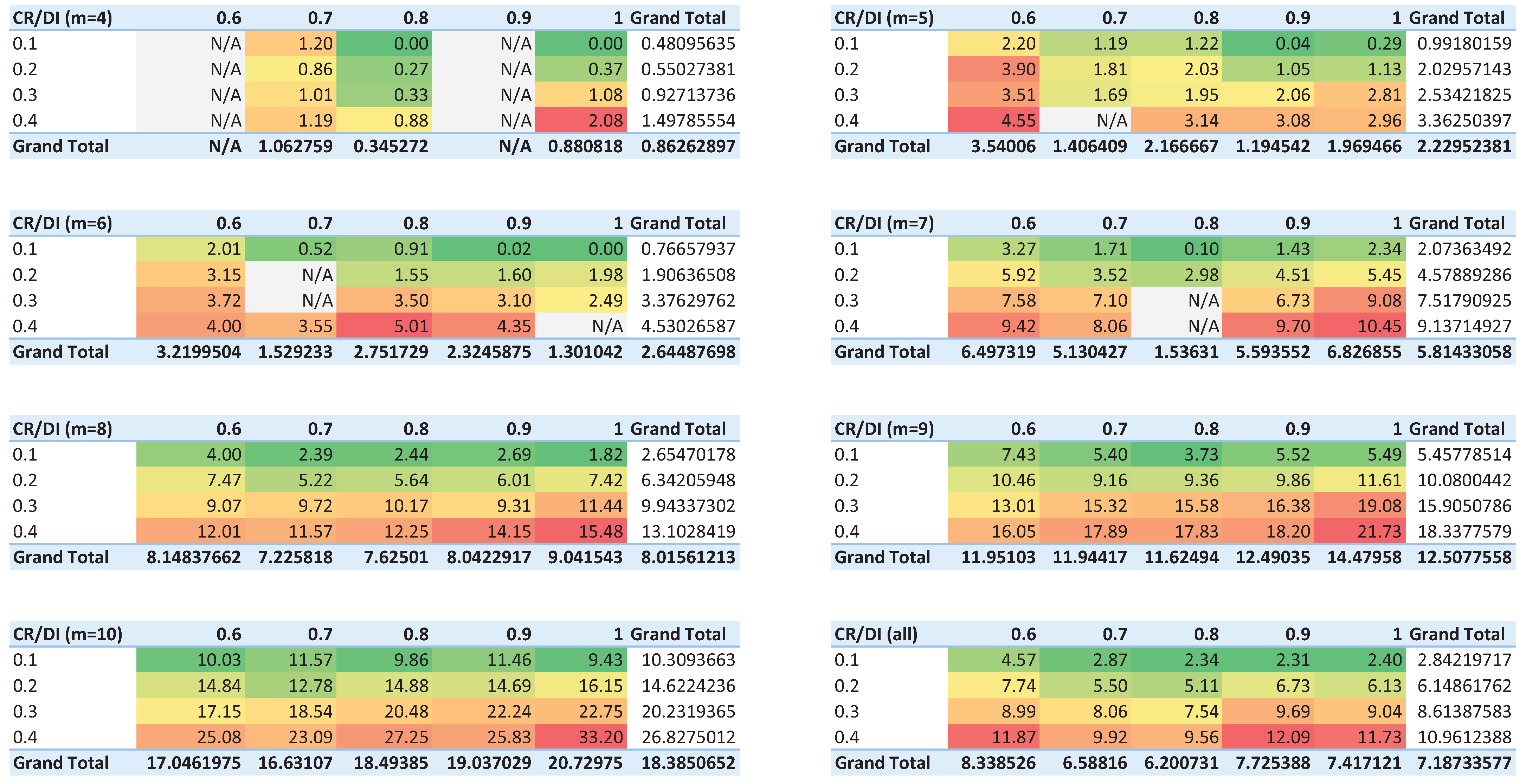
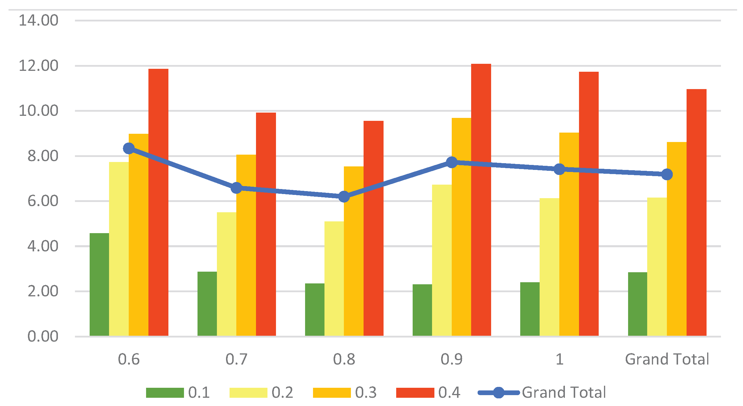
In our synthetic experiment, we arbitrarily generate values for UTs of length t (and according to possible values from $dict$ that also may repeat within one UT) and then reconstruct PCMs accordingly.

We introduce optimization that regulates the initial values of the CR and DI parameters (before optimization). For the initial values of $C{R}_{bef}$, we took $ls{t}_a=[0.1,0.2,0.3,0.4]$. For the initial values of $D{I}_{bef}$, we took $ls{t}_b=[0.6,0.7,0.8,0.9,1]$. For a in $ls{t}_a$ and b in $ls{t}_b$, we can define the following goal function ($f_e$) that we want to minimize:

$$\left(min\right)f_e=\left|C{R}_{bef}-a\right|+\left|D{I}_{bef}-b\right|.$$

(17)

We synthetically generate the sensitive column (with m rows) so that in its first half are discriminated alternatives ($s=1$), and in the second half are the privileged ones ($s=0$).

We also chose the same GA package (as explained in the previous section) to solve this unconstrained optimization. The optimization solution is the vector of preferences/estimates in the UT of matrix A, which gives the required combination of CR and DI parameters.

Setting the initial parameters ${CR}_{bef}$ and ${DI}_{bef}$ was always successful, but with some inaccuracies (that we tend to minimize). They are related to the limited possibilities of precise adjustment of the initial parameters, especially regarding a smaller number of alternatives. Specifically, when rounding, the target values may fall into the adjacent category (e.g., for $m=4$, instead of initially predefined category ${DI}_{bef}=0.6$, the value 0.667 falls in category ${DI}_{bef}=0.7$).

Following $f_e$-related optimization, we continue with the discrete ($f_d$) optimization. The lists of initial parameters ($ls{t}_a$ and $ls{t}_b$) generate 20 required combinations. Further, we assign that each combination repeats 20 times, including seven different matrix sizes ($4\le m\le 10$), resulting in 2800 optimization runs.

3. Results

Table 4. Percentages of successfully solved discrete optimizations by PCM size.

PCM Size (m)	Percentage
4	100.00%
5	100.00%
6	100.00%
7	99.5%
8	99.25%
9	98.25%
10	99.5%
Total	99.5%

shows percentages of successfully solved discrete optimization (with $f_d$ objective function) by PCM size. Except for one failed optimization concerning the ${CR}_{aft}$ parameter constraint (for $m=10$), all other failed optimizations are due to the failure of the ${DI}_{aft}$ parameter constraints (rounded ${DI}_{bef}=0.6$ in all the cases). The future results only refer to successful discrete optimizations (for which ${\overline{DI}}_{aft}=0.9289$).

Proof of Hypothesis 1.

The experimental results confirm that it is possible to correct initial AHP PCMs to be fair and consistent (with 99.5% validity). □

Figure 1 shows average values of $f_d$ objective function after optimization (i.e., sacrificed accuracy of initial PCMs) for different matrix sizes separately ($m=4,5,6,\cdots ,10$), depending on the predefined combinations of parameters CR and DI (i.e., ${CR}_{bef}$- and ${DI}_{bef}$-values). The last table (marked as all) summarizes the results for all considered PCM sizes. Missing values (N/A) result from inaccuracy in rounding the parameters resulting from the optimization in the synthetic experiment.

Colors range from deep green (most desirable values), through yellow and orange, to deep red (least desirable values), suggesting the suitability of the goal function, given the anticipated minimization of changes. The Grand Total covers the total observed average value, regardless of segmented categories.

Figure 2 compares average values of $f_d$ objective function (y-axis) for different values of the initial DI (x-axis) and CR (colors in legend). It includes all considered PCM sizes and the Grand Total results. When the starting point is high inconsistency, independent of the DI value, the average value of the goal function is more elevated, i.e., the conclusion is that it is more challenging to correct the consistency issue.

4. Discussion

The proposed method follows a postprocessing procedure to minimize changes from initial settings regarding DMs’ judgments to avoid inconsistency and discrimination toward vulnerable groups. Minimizing deviation norms for deriving priority vectors (i.e., weights) because of inconsistent DMs’ judgments in AHP pairwise comparisons is present in [79]. While our method represents a trade-off between consistency and fairness, Benítez et al. [80] introduce a framework for balancing consistency and expert judgment.

Inconsistency, especially transitivity failure and related paradoxes, is an issue of many pairwise comparison methods for decision-making related to ranking and voting systems (such as the Condorcet method, Copeland’s method, etc.) [81]. Relative to the initial CR conditions, we experimentally concluded that consistency is harder to fix in AHP PCMs with a size greater than 6. Hence, we use our method with a starting point from the consistent matrix.

The values of objective functions for discrete optimization proportionally increase with the larger PCM sizes and unfavorable initial CR conditions. Regarding the initial level of DI, our $pen2$ and $pen3$ functions in fairness constraints were constant zeros. Still, with more biased initial data, there is a smaller percentage of successfully solved controls (for example, it equals 79.52% for $D{I}_{bef}=0.5$).

We use a k-step iterative method for determining weights (k is not fixed, i.e., it fits until stabilization of priorities, Equation (7)) and an eigenvector method for checking the consistency (Equation (8)), while other approaches are also possible. For example, it is possible to use an approximate technique [82] to determine the weights, i.e., the first pass calculation only (without iteration, as in Equation (2)) that gives w, and Rayleigh quotient (RQ) to check the consistency (according to the following formula: $\lambda =\frac{Aw\ast w}{w\ast w}$). Usage of the geometric mean method [83] and many other consistency indices (in addition to Equation (4)) summarized by Pant et al. [40] is also possible.

For 100 synthetically generated matrices of size $m=10$, with the following initial conditions: $C{R}_{bef}\approx 0.2$, $D{I}_{bef}\approx 0.7$ (similar as in Section 2.3), we initiate 100 optimization runs by the two approaches (iterative–eigenvector vs. approximate–RQ) and compare the obtained results in

Table 5. Comparison of two approaches: iterative–eigenvector vs. approximate–RQ.

Approach	Successful Optimizations (in%)	$\overline{{\mathit{f}}_{\mathit{d}}}$	${\overline{\mathbf{CR}}}_{\mathbf{aft}}$	${\overline{\mathbf{DI}}}_{\mathbf{aft}}$
Iterative–eigenvector	99.00%	13.6658	0.0939	0.8476
Approximate–RQ	86.00%	12.4885	0.0943	0.8499

Bolded values are preferable.

. Because the iterative–eigenvector approach results in significantly different initial inconsistency for the same data (i.e., synthetically generated matrices A) compared with the approximate–RQ approach (for which $C{R}_{bef}$-values are considerably larger), we separately generate two datasets with similar starting points. For the iterative–eigenvector approach, ${\overline{CR}}_{bef}=0.2014$ and ${\overline{DI}}_{bef}=0.7172$; for the approximate–RQ approach, ${\overline{CR}}_{bef}=0.2167$ and ${\overline{DI}}_{bef}=0.7121$. The results only refer to successful $f_d$ optimizations (bolded values are preferable: maximal number of successful optimizations, minimal $\overline{f_d}$, minimal ${\overline{CR}}_{aft}$, and ${\overline{DI}}_{aft}$ closer to 1).

In both compared approaches, we use our advanced procedure (substantiated by Theorem 1) to improve consistency. The results show that the iterative–eigenvector approach results in a significantly higher percentage of successfully performed optimizations.

5. Conclusions

The introduced methodology has two-folded main contributions. Firstly, it solved one mature issue in AHP PCMs related to logical inconsistency in DMs’ judgments. Secondly, compared with other methods that deal only with the question of consistency, it can also deal with fairness constraints and satisfy new trends related to the need for unbiased algorithmic decision-making. Automated corrections of human DMs’ judgments with anti-discriminatory components embedded enable us to achieve fairness and consistency simultaneously (or to improve one of these fields and not disrupt the other).

When fairness meets consistency, two groups of nonlinear constraints are faced. Instead of causing numerical bifurcations in searching space (as described in different models [84,85,86]), our suggested model successfully finds winning combinations (we experimentally confirmed our research hypothesis in a large percentage, i.e., 99.5% concerning observed 2800 optimization runs). The method’s advantage is the possibility of performing discrete optimization procedures with predefined Saaty’s scale to minimize deviations from initial PCMs. Our suggested technique that starts from consistent matrices is suitable to avoid inconsistency (especially in combination with the iterative–eigenvector approach). Although the method simultaneously repairs DI when comparing alternatives in pairs, very biased matrices are harder to fix.

Some possible future research directions can be as follows:

• Expanding and applying the methodology to the whole AHP hierarchy structure;
• Fixing some judgments that DMs do not want to change;
• Setting multiobjective discrete optimizations (such as in [87]) to achieve additional goals (regarding AHP hierarchy structure or the used accuracy/fairness metrics).

Limitations of the study are primarily related to the boundaries of classical AHP methodology and, therefore, a small number of comparison alternatives and the impossibility of exploring and optimizing fairness metrics in a real data mining context.

References

1. Saaty, R.W. The analytic hierarchy process—What it is and how it is used. Math. Model. 1987, 9, 161–176. [Google Scholar] [CrossRef] [Green Version]
2. de FSM Russo, R.; Camanho, R. Criteria in AHP: A systematic review of literature. Procedia Comput. Sci. 2015, 55, 1123–1132. [Google Scholar] [CrossRef] [Green Version]
3. Cabała, P. Using the analytic hierarchy process in evaluating decision alternatives. Oper. Res. Decis. 2010, 20, 5–23. [Google Scholar]
4. Vaidya, O.S.; Kumar, S. Analytic hierarchy process: An overview of applications. Eur. J. Oper. Res. 2006, 169, 1–29. [Google Scholar] [CrossRef]
5. Darko, A.; Chan, A.P.C.; Ameyaw, E.E.; Owusu, E.K.; Parn, E.; Edwards, D.J. Review of application of analytic hierarchy process (AHP) in construction. Int. J. Constr. Manag. 2019, 19, 436–452. [Google Scholar] [CrossRef]
6. Al-Harbi, K.M.A.S. Application of the AHP in project management. Int. J. Proj. Manag. 2001, 19, 19–27. [Google Scholar] [CrossRef]
7. Subramanian, N.; Ramanathan, R. A review of applications of Analytic Hierarchy Process in operations management. Int. J. Prod. Econ. 2012, 138, 215–241. [Google Scholar] [CrossRef]
8. Liberatore, M.J.; Nydick, R.L. The analytic hierarchy process in medical and health care decision making: A literature review. Eur. J. Oper. Res. 2008, 189, 194–207. [Google Scholar] [CrossRef]
9. Ruiz Bargueño, D.; Salomon, V.A.P.; Marins, F.A.S.; Palominos, P.; Marrone, L.A. State of the art review on the analytic hierarchy process and urban mobility. Mathematics 2021, 9, 3179. [Google Scholar] [CrossRef]
10. Saaty, T.L. A scaling method for priorities in hierarchical structures. J. Math. Psychol. 1977, 15, 234–281. [Google Scholar] [CrossRef]
11. Munier, N.; Hontoria, E. Uses and Limitations of the AHP Method; Springer: Cham, Switzerland, 2021. [Google Scholar]
12. Kwiesielewicz, M.; Van Uden, E. Inconsistent and contradictory judgements in pairwise comparison method in the AHP. Comput. Oper. Res. 2004, 31, 713–719. [Google Scholar] [CrossRef]
13. Bozóki, S.; Fulop, J.; Poesz, A. On reducing inconsistency of pairwise comparison matrices below an acceptance threshold. Cent. Eur. J. Oper. Res. 2015, 23, 849–866. [Google Scholar] [CrossRef] [Green Version]
14. Pereira, V.; Costa, H.G. Nonlinear programming applied to the reduction of inconsistency in the AHP method. Ann. Oper. Res. 2015, 229, 635–655. [Google Scholar] [CrossRef]
15. Zhang, Y.; Bellamy, R.; Varshney, K. Joint optimization of AI fairness and utility: A human-centered approach. In Proceedings of the Proceedings of the AAAI/ACM Conference on AI, Ethics, and Society, New York, NY, USA, 7–9 February 2020; pp. 400–406. [Google Scholar] [CrossRef] [Green Version]
16. Dodevska, Z.; Petrović, A.; Radovanović, S.; Delibašić, B. Changing criteria weights to achieve fair VIKOR ranking: A postprocessing reranking approach. Auton. Agents Multi-Agent Syst. 2023, 37, 1–44. [Google Scholar] [CrossRef]
17. Chen, C.; Cook, W.D.; Imanirad, R.; Zhu, J. Balancing Fairness and Efficiency: Performance Evaluation with Disadvantaged Units in Non-homogeneous Environments. Eur. J. Oper. Res. 2020, 287, 1003–1013. [Google Scholar] [CrossRef]
18. Radovanović, S.; Petrović, A.; Delibašić, B.; Suknović, M. Eliminating Disparate Impact in MCDM: The case of TOPSIS. In Proceedings of the Central European Conference on Information and Intelligent Systems, Varaždin, Croatia, 13–15 October 2021; pp. 275–282. [Google Scholar]
19. Çakır, O.; Gurler, İ.; Gunduzyeli, B. Analysis of a Non-Discriminating Criterion in Simple Additive Weighting Deep Hierarchy. Mathematics 2022, 10, 3192. [Google Scholar] [CrossRef]
20. Askarisichani, O.; Bullo, F.; Friedkin, N.E.; Singh, A.K. Predictive models for human–AI nexus in group decision making. Ann. N. Y. Acad. Sci. 2022, 1514, 70–81. [Google Scholar] [CrossRef]
21. Bastani, H.; Bastani, O.; Sinchaisri, W.P. Improving human decision-making with machine learning. arXiv 2021, arXiv:2108.08454. [Google Scholar] [CrossRef]
22. Jago, A.S.; Laurin, K. Assumptions about algorithms’ capacity for discrimination. Personal. Soc. Psychol. Bull. 2022, 48, 582–595. [Google Scholar] [CrossRef]
23. Pessach, D.; Shmueli, E. Improving fairness of artificial intelligence algorithms in Privileged-Group Selection Bias data settings. Expert Syst. Appl. 2021, 185, 115667. [Google Scholar] [CrossRef]
24. Kordzadeh, N.; Ghasemaghaei, M. Algorithmic bias: Review, synthesis, and future research directions. Eur. J. Inf. Syst. 2022, 31, 388–409. [Google Scholar] [CrossRef]
25. Rambachan, A.; Roth, J. Bias in, bias out? Evaluating the folk wisdom. arXiv 2019, arXiv:1909.08518. [Google Scholar]
26. Cecere, G.; Corrocher, N.; Jean, C. Fair or Unbiased Algorithmic Decision-Making? A Review of the Literature on Digital Economics. In A Review of the Literature on Digital Economics (October 15, 2021); SSRN: Rochester, NY, USA, 2021. [Google Scholar] [CrossRef]
27. Tolan, S. Fair and unbiased algorithmic decision making: Current state and future challenges. arXiv preprint 2019, arXiv:1901.04730. [Google Scholar]
28. Hakli, H.; Uguz, H.; Ortacay, Z. Comparing the performances of six nature-inspired algorithms on a real-world discrete optimization problem. Soft Comput. 2022, 26, 11645–11667. [Google Scholar] [CrossRef]
29. Hajian, S.; Domingo-Ferrer, J. A methodology for direct and indirect discrimination prevention in data mining. IEEE Trans. Knowl. Data Eng. 2012, 25, 1445–1459. [Google Scholar] [CrossRef]
30. Zliobaite, I. A survey on measuring indirect discrimination in machine learning. arXiv 2015, arXiv:1511.00148. [Google Scholar]
31. Bennett, C.; Keyes, O. What is the point of fairness? Interactions 2020, 27, 35–39. [Google Scholar] [CrossRef]
32. Hacker, P. Teaching fairness to artificial intelligence: Existing and novel strategies against algorithmic discrimination under EU law. Common Mark. Law Rev. 2018, 55, 1143–1185. [Google Scholar] [CrossRef]
33. Madzík, P.; Falát, L. State-of-the-art on analytic hierarchy process in the last 40 years: Literature review based on Latent Dirichlet Allocation topic modelling. PLoS ONE 2022, 17, e0268777. [Google Scholar] [CrossRef]
34. Emrouznejad, A.; Marra, M. The state of the art development of AHP (1979–2017): A literature review with a social network analysis. Int. J. Prod. Res. 2017, 55, 6653–6675. [Google Scholar] [CrossRef] [Green Version]
35. Yu, D.; Kou, G.; Xu, Z.; Shi, S. Analysis of collaboration evolution in AHP research: 1982–2018. Int. J. Inf. Technol. Decis. Mak. 2021, 20, 7–36. [Google Scholar] [CrossRef]
36. Kong, F.; Liu, H. An improvement on Saaty’s AHP. In Proceedings of the IFIP International Conference on Artificial Intelligence Applications and Innovations, Beijing, China, 7–9 September 2005; pp. 301–312. [Google Scholar] [CrossRef]
37. Lootsma, F.A. The Additive and the Multiplicative AHP. In Fuzzy Logic for Planning and Decision Making; Springer: New York, NY, USA, 1997; pp. 109–147. [Google Scholar] [CrossRef]
38. Maleki, H.; Zahir, S. A comprehensive literature review of the rank reversal phenomenon in the analytic hierarchy process. J. Multi-Criteria Decis. Anal. 2013, 20, 141–155. [Google Scholar] [CrossRef]
39. Munier, N.; Hontoria, E. Shortcomings of the AHP Method. In Uses and limitations of the AHP Method; Springer: Cham, Switzerland, 2021; pp. 41–90. [Google Scholar] [CrossRef]
40. Pant, S.; Kumar, A.; Ram, M.; Klochkov, Y.; Sharma, H.K. Consistency Indices in Analytic Hierarchy Process: A Review. Mathematics 2022, 10, 1206. [Google Scholar] [CrossRef]
41. Mardani, A.; Zavadskas, E.K.; Govindan, K.; Amat Senin, A.; Jusoh, A. VIKOR technique: A systematic review of the state of the art literature on methodologies and applications. Sustainability 2016, 8, 37. [Google Scholar] [CrossRef] [Green Version]
42. Sangiorgio, V.; Uva, G.; Fatiguso, F. Optimized AHP to overcome limits in weight calculation: Building performance application. J. Constr. Eng. Manag. 2018, 144, 04017101. [Google Scholar] [CrossRef]
43. Ishizaka, A.; Pearman, C.; Nemery, P. AHPSort: An AHP-based method for sorting problems. Int. J. Prod. Res. 2012, 50, 4767–4784. [Google Scholar] [CrossRef] [Green Version]
44. Ishizaka, A.; López, C. Cost-benefit AHPSort for performance analysis of offshore providers. Int. J. Prod. Res. 2019, 57, 4261–4277. [Google Scholar] [CrossRef]
45. Li, F.; Phoon, K.K.; Du, X.; Zhang, M. Improved AHP method and its application in risk identification. J. Constr. Eng. Manag. 2013, 139, 312–320. [Google Scholar] [CrossRef] [Green Version]
46. Lin, C.C.; Wang, W.C.; Yu, W.D. Improving AHP for construction with an adaptive AHP approach (A3). Autom. Constr. 2008, 17, 180–187. [Google Scholar] [CrossRef]
47. Xiulin, S.; Dawei, L. An improvement analytic hierarchy process and its application in teacher evaluation. In Proceedings of the 2014 Fifth International Conference on Intelligent Systems Design and Engineering Applications, Zhangjiajie, China, 15–16 June 2014; pp. 169–172. [Google Scholar] [CrossRef]
48. Leal, J.E. AHP-express: A simplified version of the analytical hierarchy process method. MethodsX 2020, 7, 100748. [Google Scholar] [CrossRef]
49. Chen, T. A diversified AHP-tree approach for multiple-criteria supplier selection. Comput. Manag. Sci. 2021, 18, 431–453. [Google Scholar] [CrossRef]
50. Abastante, F.; Corrente, S.; Greco, S.; Ishizaka, A.; Lami, I.M. A new parsimonious AHP methodology: Assigning priorities to many objects by comparing pairwise few reference objects. Expert Syst. Appl. 2019, 127, 109–120. [Google Scholar] [CrossRef] [Green Version]
51. Nefeslioglu, H.A.; Sezer, E.A.; Gokceoglu, C.; Ayas, Z. A modified analytical hierarchy process (M-AHP) approach for decision support systems in natural hazard assessments. Comput. Geosci. 2013, 59, 1–8. [Google Scholar] [CrossRef]
52. Tesfamariam, S.; Sadiq, R. Risk-based environmental decision-making using fuzzy analytic hierarchy process (F-AHP). Stoch. Environ. Res. Risk Assess. 2006, 21, 35–50. [Google Scholar] [CrossRef]
53. Bañuelas, R.; Antony, J. Modified analytic hierarchy process to incorporate uncertainty and managerial aspects. Int. J. Prod. Res. 2004, 42, 3851–3872. [Google Scholar] [CrossRef]
54. Xu, S.; Xu, D.; Liu, L. Construction of regional informatization ecological environment based on the entropy weight modified AHP hierarchy model. Sustain. Comput. Informatics Syst. 2019, 22, 26–31. [Google Scholar] [CrossRef]
55. Sadiq, R.; Tesfamariam, S. Environmental decision-making under uncertainty using intuitionistic fuzzy analytic hierarchy process (IF-AHP). Stoch. Environ. Res. Risk Assess. 2009, 23, 75–91. [Google Scholar] [CrossRef]
56. Lin, K.; Chen, H.; Xu, C.Y.; Yan, P.; Lan, T.; Liu, Z.; Dong, C. Assessment of flash flood risk based on improved analytic hierarchy process method and integrated maximum likelihood clustering algorithm. J. Hydrol. 2020, 584, 124696. [Google Scholar] [CrossRef]
57. Deng, X.; Hu, Y.; Deng, Y.; Mahadevan, S. Supplier selection using AHP methodology extended by D numbers. Expert Syst. Appl. 2014, 41, 156–167. [Google Scholar] [CrossRef]
58. Gao, R.; Shah, C. Toward creating a fairer ranking in search engine results. Inf. Process. Manag. 2020, 57, 102138. [Google Scholar] [CrossRef]
59. Mehrabi, N.; Morstatter, F.; Saxena, N.; Lerman, K.; Galstyan, A. A survey on bias and fairness in machine learning. ACM Comput. Surv. (CSUR) 2021, 54, 1–35. [Google Scholar] [CrossRef]
60. Verma, S.; Rubin, J. Fairness definitions explained. In Proceedings of the 2018 IEEE/ACM International Workshop on Software Fairness (Fairware), Gothenburg, Sweden, 29 May 2018; pp. 1–7. [Google Scholar] [CrossRef]
61. Narayanan, A. Translation tutorial: 21 fairness definitions and their politics. In Proceedings of the Conference Fairness Accountability, and Transparency New York, NY, USA, 23–24 February 2018; Volume 1170, p. 3. [Google Scholar]
62. Rabiee, M.; Aslani, B.; Rezaei, J. A decision support system for detecting and handling biased decision-makers in multi criteria group decision-making problems. Expert Syst. Appl. 2021, 171, 114597. [Google Scholar] [CrossRef]
63. Opricovic, S. A compromise solution in water resources planning. Water Resour. Manag. 2009, 23, 1549–1561. [Google Scholar] [CrossRef]
64. Fu, C.; Zhou, K.; Xue, M. Fair framework for multiple criteria decision making. Comput. Ind. Eng. 2018, 124, 379–392. [Google Scholar] [CrossRef]
65. Pager, D.; Shepherd, H. The sociology of discrimination: Racial discrimination in employment, housing, credit, and consumer markets. Annu. Rev. Sociol. 2008, 34, 181. [Google Scholar] [CrossRef] [Green Version]
66. Nuseir, M.T.; Al Kurdi, B.H.; Alshurideh, M.T.; Alzoubi, H.M. Gender discrimination at workplace: Do Artificial Intelligence (AI) and Machine Learning (ML) have opinions about it. In Proceedings of the The International Conference on Artificial Intelligence and Computer Vision, Settat, Morocco, 28–30 June 2021; pp. 301–316. [Google Scholar] [CrossRef]
67. Macnicol, J. Age Discrimination: An Historical and Contemporary Analysis; Cambridge University Press: Cambridge, UK, 2006. [Google Scholar]
68. Uccellari, P. Multiple discrimination: How law can reflect reality. Equal. Rights Rev. 2008, 1, 24–49. [Google Scholar]
69. Ghosh, A.; Dutt, R.; Wilson, C. When fair ranking meets uncertain inference. In Proceedings of the Proceedings of the 44th International ACM SIGIR Conference on Research and Development in Information Retrieval, Virtual Event, 11–15 July 2021; pp. 1033–1043. [Google Scholar] [CrossRef]
70. Liberatore, M.J.; Nydick, R.L. Wash criteria and the analytic hierarchy process. Comput. Oper. Res. 2004, 31, 889–892. [Google Scholar] [CrossRef]
71. Barocas, S.; Selbst, A.D. Big data’s disparate impact. Calif. Law Rev. 2016, 104, 671. [Google Scholar] [CrossRef]
72. Besse, P.; del Barrio, E.; Gordaliza, P.; Loubes, J.M.; Risser, L. A survey of bias in machine learning through the prism of statistical parity. Am. Stat. 2022, 76, 188–198. [Google Scholar] [CrossRef]
73. Feldman, M.; Friedler, S.A.; Moeller, J.; Scheidegger, C.; Venkatasubramanian, S. Certifying and removing disparate impact. In Proceedings of the 21th ACM SIGKDD International Conference on Knowledge Discovery and Data Mining, Sydney, Australia, 10–13 August 2015; pp. 259–268. [Google Scholar] [CrossRef] [Green Version]
74. Katoch, S.; Chauhan, S.S.; Kumar, V. A review on genetic algorithm: Past, present, and future. Multimed. Tools Appl. 2021, 80, 8091–8126. [Google Scholar] [CrossRef]
75. Mirjalili, S. Genetic algorithm. In Evolutionary Algorithms and Neural Networks; Springer: Cham, Switzerland, 2019; pp. 43–55. [Google Scholar] [CrossRef]
76. Lee, C.K.H. A review of applications of genetic algorithms in operations management. Eng. Appl. Artif. Intell. 2018, 76, 1–12. [Google Scholar] [CrossRef]
77. Slowik, A.; Kwasnicka, H. Evolutionary algorithms and their applications to engineering problems. Neural Comput. Appl. 2020, 32, 12363–12379. [Google Scholar] [CrossRef] [Green Version]
78. Solgi, R.M. MIT License Geneticalgorithm 1.0.2. Available online: https://pypi.org/project/geneticalgorithm/ (accessed on 27 November 2022).
79. Zhang, J.; Kou, G.; Peng, Y.; Zhang, Y. Estimating priorities from relative deviations in pairwise comparison matrices. Inf. Sci. 2021, 552, 310–327. [Google Scholar] [CrossRef]
80. Benítez, J.; Delgado-Galván, X.; Gutiérrez, J.A.; Izquierdo, J. Balancing consistency and expert judgment in AHP. Math. Comput. Model. 2011, 54, 1785–1790. [Google Scholar] [CrossRef]
81. Kułakowski, K. Inconsistency in the ordinal pairwise comparisons method with and without ties. Eur. J. Oper. Res. 2018, 270, 314–327. [Google Scholar] [CrossRef] [Green Version]
82. Ishizaka, A.; Nemery, P. Multi-Criteria Decision Analysis: Methods and Software; John Wiley & Sons: Hoboken, NJ, USA, 2013. [Google Scholar]
83. Crawford, G.; Williams, C. A note on the analysis of subjective judgment matrices. J. Math. Psychol. 1985, 29, 387–405. [Google Scholar] [CrossRef]
84. Li, B.; Liang, H.; He, Q. Multiple and generic bifurcation analysis of a discrete Hindmarsh-Rose model. Chaos Solitons Fractals 2021, 146, 110856. [Google Scholar] [CrossRef]
85. Eskandari, Z.; Avazzadeh, Z.; Khoshsiar Ghaziani, R.; Li, B. Dynamics and bifurcations of a discrete-time Lotka–Volterra model using nonstandard finite difference discretization method. Math. Methods Appl. Sci. 2022. [Google Scholar] [CrossRef]
86. Li, B.; Liang, H.; Shi, L.; He, Q. Complex dynamics of Kopel model with nonsymmetric response between oligopolists. Chaos Solitons Fractals 2022, 156, 111860. [Google Scholar] [CrossRef]
87. Liu, Q.; Li, X.; Liu, H.; Guo, Z. Multi-objective metaheuristics for discrete optimization problems: A review of the state-of-the-art. Appl. Soft Comput. 2020, 93, 106382. [Google Scholar] [CrossRef]
Figure 1. Average values of f d objective function for different PCM sizes observed concerning predefined combinations of CR and DI.
Mathematics 11 00604 g001
Figure 2. Comparison of average values of f d objective function for different values of the initial DI and CR set-points.
Mathematics 11 00604 g002