Article

Analytical Description of the Diffusion in a Cellular Automaton with the Margolus Neighbourhood in Terms of the Two-Dimensional Markov Chain

by
Anton E. Kulagin
1,*,† and
Alexander V. Shapovalov
2,3,*,†
1
Division for Electronic Engineering, Tomsk Polytechnic University, 30 Lenina av., 634050 Tomsk, Russia
2
Department of Theoretical Physics, Tomsk State University, 1 Novosobornaya Sq., 634050 Tomsk, Russia
3
Laboratory for Theoretical Cosmology, International Centre of Gravity and Cosmos, Tomsk State University of Control Systems and Radioelectronics, 40 Lenina av., 634050 Tomsk, Russia
*
Authors to whom correspondence should be addressed.
These authors contributed equally to this work.
Mathematics 2023, 11(3), 584; https://doi.org/10.3390/math11030584
Submission received: 30 December 2022 / Revised: 19 January 2023 / Accepted: 19 January 2023 / Published: 22 January 2023

Abstract

:
The one-parameter two-dimensional cellular automaton with the Margolus neighbourhood is analyzed based on considering the projection of the stochastic movements of a single particle. Introducing the auxiliary random variable associated with the direction of the movement, we reduce the problem under consideration to the study of a two-dimensional Markov chain. The master equation for the probability distribution is derived and solved exactly using the probability-generating function method. The probability distribution is expressed analytically in terms of Jacobi polynomials. The moments of the obtained solution allowed us to derive the exact analytical formula for the parametric dependence of the diffusion coefficient in the two-dimensional cellular automaton with the Margolus neighbourhood. Our analytic results agree with earlier empirical results of other authors and refine them. The results are of interest for the modelling two-dimensional diffusion using cellular automata especially for the multicomponent problem.

1. Introduction

Cellular automata (CA) are a powerful tool for modelling matter transport [1]. The attractive feature of CA is that contemporary algorithms of parallel computing can be naturally embedded in them. Various cellular algorithms were successfully implemented on field-programmable gate arrays (FPGA) [2,3] and on graphic cards [4,5].
In the study of diffusion phenomena in physics, chemistry, and biology, CA are positioned as one of the effective tools for modelling systems of many particles. The simplest CA with boolean alphabet modelling the diffusion are the asynchronous CA with naive diffusion and the synchronous CA with Margolus neighbourhood [6] or briefly Margolus CA (MCA). The last one is the object of our study. Exactly this type of the CA attracted our attention since synchronous CA are more advantageous in terms of the computing speed (see, e.g., comparison in [7]). Note that the MCA is representative of partitioning CA.
The most common macroscopic characteristics of the diffusion transfer is the diffusion coefficient D c that is defined as the proportionality factor in Fick’s law [8,9]. The diffusion coefficient is usually invariant when the movements of particles are caused just by random fluctuations rather than by any fields. Nevertheless, the processes with the time-dependent diffusion coefficient are also of interest, e.g., in the ambipolar diffusion phenomena [10,11,12]. The most popular model of the diffusion is the kinetic model, which is based on a differential equations that can be solved, for example, using difference schemes [13,14,15]. In such approach, the diffusion coefficient is an explicit parameter of the model. For cellular automata, the diffusion coefficient is not presented in the model explicitly. Calculating the diffusion coefficient for the CA with naive diffusion is a trivial task since it directly models the random walk of particles that is well-studied. However, it is not trivial for partitioning CA including MCA. We show here that the diffusion in the two-dimensional MCA can be described in terms of one two-dimensional Markov chain as opposed to the one-dimensional random walk. In our paper, we study the exact solution of this two-dimensional Markov chain whose characteristics are crucial for the mathematical description of the diffusion in MCA.
While multidimensional Markov chains arise in a number of applications in service theory [16], genetic networks [17], Gibbs sampling [18], and other areas [19], there are very few exactly solvable multidimensional Markov chains that do not degenerate to the one-dimensional one. Therefore, the exact solutions to the two-dimensional Markov chain under consideration can be of interest for specialists in applied mathematics and useful for applications other than cellular automaton theory.
The paper is organized as follows. In Section 2, we describe the diffusion model within the framework of the two-dimensional cellular automata with Margolus neighbourhood. Furthermore, we explain the way of obtaining the diffusion coefficient for this model based on the considering one-dimensional movement of a single particle. In Section 3, the stochastic process describing the one-dimensional movement of a single particle is given. The idea of introducing the auxiliary random variable associated with the direction of movement is proposed. This approach allows us to consider the process under consideration as the two-dimensional Markov chain. In Section 4, the formal mathematical definition of this chain and basic notations are given. In Section 5, we solve the master equation for the probability distribution of the particle coordinate using the probability generating function method. The moments of this distribution are derived. In Section 6, the obtained results are discussed within the framework of the diffusion model. The exact analytical formula for the diffusion coefficient is derived, and properties of the cellular automaton with the Margolus neighbourhood are discussed. In Section 7, we conclude with some remarks.

2. Diffusion in the Margolus Cellular Automaton

In the two-dimensional cellular automata with Margolus neighbourhood, the diffusion is described based on the following algorithm [6]:
(1) The plane is divided into identical square cells forming a cell grid. One cell contains a boolean variable that takes the value 0 or 1 corresponding to the absence or presence of a particle in the cell, respectively.
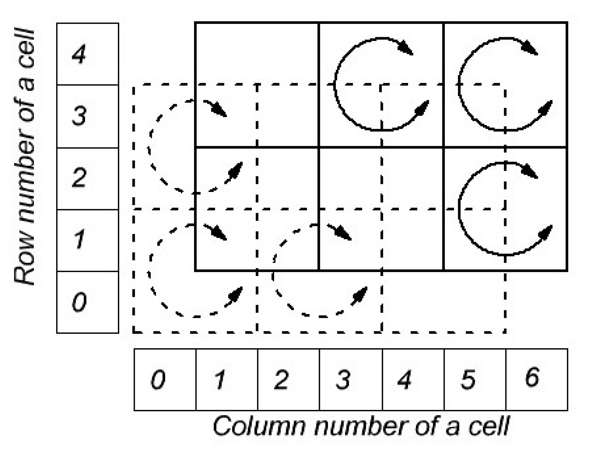
(2) The cell grid is divided into blocks of 2 × 2 cells. Such partition can be even or odd (see Figure 1). The even partition corresponds to the case when the left lower cell of each block has even vertical and horizontal numbers. The odd partition corresponds to the case when the left lower cell of each block has odd vertical and horizontal numbers.
(3) Beginning from an initial state, on each discrete time step the following rule is applied to each block independently. We rotate the block 90 clockwise or counterclockwise with the probability of 0 < p 0.5 for each outcome. The rule is applied to blocks of the even partition on even time steps and it is applied to blocks of the odd partition on odd time steps. If each time step corresponds to the same time interval Δ t and p = const , then such MCA simulates the diffusion with the time independent diffusion coefficient D c .
The classic MCA uses p = 0.5 , i.e., blocks always rotate. In such approach, the diffusion rate is controlled with the length of the time interval corresponding to one discrete time step and with the size of a cell. However, this model can be applied to the multicomponent diffusion problem. In this case, the cell contains few bits that correspond to particles of different substances. It can be treated as few layers of the cell grid. Then, we can not directly apply the described rule with p = 0.5 for every layer of particles if the diffusion rates for these substances are not equal. The difference in diffusion rates can be realized using different p for different substances. The only drawback of such approach is that the diffusion coefficient D c = D c ( p ) nonlinearly depends on p. The other way is using the same p = 0.5 for each layer but skip two consecutive time steps for one or few layers with a probability equal to p s (the rotation rule is not applied to any blocks of the respective layer on the skipped time step). In this approach, the diffusion coefficient linearly depends on p s . The differences between these two approaches will be discussed in Section 6.
In order to model the diffusion using the MCA, the diffusion coefficient corresponding to the particular MCA must be determined. It can be shown (see, e.g., [20]) that
D c ( p ) = k ( p ) Δ x 2 Δ t ,
where D c ( p ) is the diffusion coefficient, Δ x is the side length of the cell, Δ t is the time interval corresponding to the discrete time step, and k ( p ) is the proportionality factor. However, relation (1) does not help to obtain the exact value of the multiplier k. Moreover, k nonlinearly depends on p as it was mentioned earlier. One way is to determine k is to compute the specific diffusion problem using the numerical realization of the MCA and to compare the result with the analytical or numerical solutions of the respective diffusion equation. Such approach allows one to find k approximately. However, it is hard to estimate the error of the obtained value. Moreover, this error depends on the choice of the specific diffusion problem. The other way is to obtain the distribution of the particle position in the MCA. Assuming that the correlation of these distributions for two particles tends to zero with the growth of time steps number, the distribution of the position of the single particle is equal to the Green function of the diffusion equation that is given by
G ( r , τ ) exp r 2 4 D c τ ,
where r is the radius vector of the particle position at time t = τ relative to the initial position at time t 0 = 0 , D c is the diffusion coefficient. For the isotropic and homogeneous problem, one can consider the projection of the particle position on one axis (let it be x). As t , the distribution of the particle position tends to the normal distribution with the probability density function given by
P X n ( x ) exp ( x M X n ) 2 2 D X n , t = n Δ t , n N ,
where X n is the random position of the particle at the n-th time step, M X n is the expectation of X n , and D X n is the dispersion of X n . Then, for Δ x = 1 , Δ t = 1 , we have
M X n 0 , n , D X n 2 n D c , n .
Hereinafter, D c will be given for Δ x = 1 , Δ t = 1 unless otherwise stated. The trick is to find the distribution P X n ( x ) or its moments analytically. In [21], the authors tried to obtain the diffusion coefficient using this approach for p = 0.5 . However, they assumed that X n is the one-dimensional Markov chain, i.e., the simplest random walk. Later on, using the software realization of MCA with higher number of cells and time steps, it was shown that this assumption led to the diffusion coefficient obtained in [21] for 2D MCA is approximately three times higher than the real one (see, e.g., [20,22,23]). However, the exact distribution of X n and the diffusion coefficient of MCA were not obtained since then. In this work, we present the exact distribution of X n in MCA and obtain the exact analytical formula of D c ( p ) for an arbitrary p including the special case p = 0.5 .

3. One-Dimensional Movement of a Single Particle

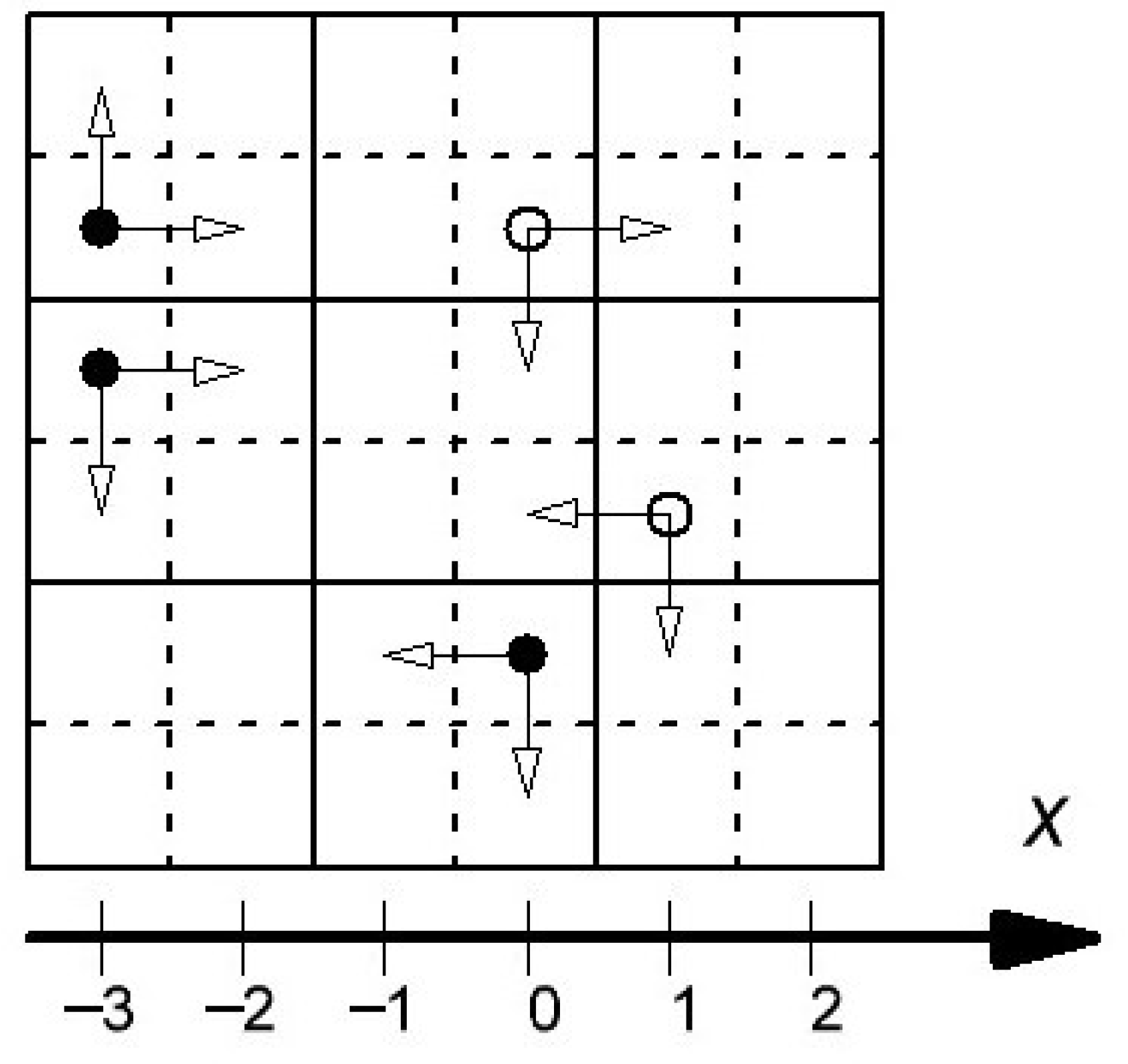
In this Section, we will describe the rules of the stochastic movement of a single particle in MCA. As it was mentioned in the previous Section, we consider the movement along the x-axis that is directed along the side of a cell. Notice that if a particle is in an odd column at an odd time step, then its x-coordinate can either increase by 1 or does not change according to the rotation rule of the MCA (see Figure 2). The same rule works for a particle in a even column at an even time step. Let the variable d show the direction of possible movement of the particle along the x-axis. If d = 1 , then x can either increase by one or does not change. If d = 1 , then x can either decrease by one or does not change. It is easy to see that d = 1 corresponds to a particle in an even column at an odd time step and to a particle in an odd column at an even time step.
Notice that the direction d does not change when the x-coordinate changes and the direction d reverts its sign when the coordinate x does not change. The first outcome is realized with the probability of p at every time step while the second outcome is realized with the probability ( 1 p ) . Note that the sequence of the x-coordinates of the single particle has a memory, i.e., the current x-coordinate of the particle depends the history of its movements. It the main issue in the analytical description of partitioning cellular automata.

4. Master Equation

Next, we give the formal definition of the two-dimensional Markov chain described in Section 3.
Let X t : Ω Z and Δ t : Ω { 1 , + 1 } be sequences of random variables where t Z + and Ω is a set of outcomes. We associate the values of X t with the discrete x-coordinate of the particle on a discrete time step t, and Δ t is associated with its direction. The probability of transitions for the chain under consideration, which were described in Section 3, are given by
Prob ( X t + 1 = X t + Δ t ; Δ t + 1 = Δ t ) = p , Prob ( X t + 1 = X t ; Δ t + 1 = Δ t ) = 1 p .
The semicolon in (5) implies the logical conjunction.
Let us denote
P t ( x , d ) = Prob ( X t = x ; Δ t = d ) .
The transition rules (5) in notations (6) yield the following master equation:
P t + 1 ( x , d ) = p P t ( x d , d ) + ( 1 p ) P t ( x , d ) .
Hereinafter, x Z , d { 1 , + 1 } , and t Z + . We consider the problem with the deterministic initial position of the particle, i.e., Prob ( X 0 = 0 ) = 1 . Then, the initial condition for (7) reads
P 0 ( x , + 1 ) = ε · δ x , 0 , P 0 ( 0 , 1 ) = ( 1 ε ) · δ x , 0 ,
where δ i , j is the Kronecker delta.
Within the framework of the diffusion problem, it is natural to consider the symmetric case P 0 ( 0 , + 1 ) = P 0 ( 0 , 1 ) . Thus, the following initial condition will be considered:
P 0 ( x , + 1 ) = δ x , 0 2 , P 0 ( x , 1 ) = δ x , 0 2 .
Since the distribution over x is of primary interest to us, we will study the marginal distribution given by
P t ( x ) = P t ( x , + 1 ) + P t ( x , 1 ) .
In order to construct the analytical description of the two-dimensional Markov chain under consideration, we will solve the master Equation (7) with the initial condition (9) in the next Section.

5. Probability Generating Function

The exact solution of (7), (9) can be derived using the method of the probability generating function [24] for the marginal distribution (10). Such probability-generating function reads
G t ( z ) = x = P t ( x ) z x .
Let us also introduce the following probability-generating functions:
G t + ( z ) = x = P t ( x , + 1 ) z x , G t ( z ) = x = P t ( x , 1 ) z x .
In view of (10), one readily gets
G t ( z ) = G t + ( z ) + G t ( z ) .
The master Equation (7) can be written as
P t + 1 ( x , + 1 ) = p P t ( x 1 , + 1 ) + ( 1 p ) P t ( x , 1 ) , P t + 1 ( x , 1 ) = p P t ( x + 1 , 1 ) + ( 1 p ) P t ( x , + 1 ) .
Multiplying the system (14) by z x and summing over x Z , we derive the following equation for the probability generating functions (12):
g t + 1 ( z ) = b ( z ) g t ( z ) , g 0 ( z ) = 1 2 1 1 , g t ( z ) = G t + ( z ) G t ( z ) , b ( z ) = p z 1 p 1 p p z 1 ,
where g 0 ( z ) is obtained from (9), (12).
The solution of the system (15) has the following form:
g t ( z ) = u ( z ) λ 1 t ( z ) 0 0 λ 2 t ( z ) u 1 ( z ) g 0 ( z ) , u ( z ) u ( z ) = u ( z ) u ( z ) = 1 ,
where the solution of the associated matrix eigenvalue problem yields
λ 1 ( z ) = p 2 z + 1 z + m ( z ) 2 , λ 2 ( z ) = p 2 z + 1 z m ( z ) 2 , u ( z ) = c 1 ( z ) ( 1 p ) c 2 ( z ) ( 1 p ) c 1 ( z ) 2 m ( z ) r ( z ) c 2 ( z ) 2 m ( z ) + r ( z ) , m ( z ) = p 2 z + 1 z 2 8 p + 4 , r ( z ) = p z 1 z , c 1 ( z ) = m ( z ) + r ( z ) 2 ( 1 p ) 2 m ( z ) , c 2 ( z ) = m ( z ) r ( z ) 2 ( 1 p ) 2 m ( z ) .
The solution (16), (17) can be rewritten as
G t + ( z ) = 1 2 m ( z ) λ 1 t ( z ) λ 2 ( z ) + λ 1 ( z ) λ 2 t ( z ) + ( 1 p + p z ) λ 1 t ( z ) λ 2 t ( z ) , G t ( z ) = 1 2 m ( z ) λ 1 t + 1 ( z ) λ 2 t + 1 ( z ) + ( 1 p p z ) λ 1 t ( z ) λ 2 t ( z ) .
Raw moments of X t for the given Δ t read
μ t ( n ) ± = x Z x n P t ( x , ± 1 ) .
The moments (19) can be obtained from
μ t ( n ) ± = d n G t ± ( z ) d z n | z = 1 .
Using (20), (18), one readily gets
μ t ( 1 ) + = μ t ( 1 ) = p 4 4 p 1 ( 2 p 1 ) t , μ t ( 2 ) + = μ t ( 2 ) = p 2 4 ( 1 p ) 2 1 + 2 ( 1 p ) p t + ( 2 p 1 ) t .
Then, the expectation M X t and the dispersion D X t of the marginal distribution (10), which are given by
M X t = x Z x P t ( x ) , D X t = x Z ( x M X t ) 2 P t ( x ) ,
read
M X t = 0 , D X t = p 2 2 ( 1 p ) 2 1 + 2 ( 1 p ) p t + ( 2 p 1 ) t , t = 0 , ¯ .
While the Formula (18) is convenient for the derivation of moments, it does not allow one to directly obtain the distribution (10). The explicit representation of the probability generating function as the power series in z is a bit tricky. The analytical form for the marginal distribution (10) is given by the following theorem.
Theorem 1. 
The marginal distribution P t ( x ) reads
P 2 n + 1 ( 2 j ) = ( 1 p ) p 2 j ( 1 2 p ) n j P n j ( 2 j , 0 ) 2 p 2 1 2 p + 1 , j = 0 , n ¯ ;
P 2 n ( 2 j ) = ( 1 p ) 2 p 2 j ( 1 2 p ) n j 1 n n j P n j 1 ( 2 j , 1 ) 2 p 2 1 2 p + 1 , j = 0 , n 1 ¯ ;
P 2 n ( 2 j + 1 ) = ( 1 p ) p 2 j + 1 ( 1 2 p ) n j 1 P n j 1 ( 2 j + 1 , 0 ) 2 p 2 1 2 p + 1 , j = 0 , n 1 ¯ ;
P 2 n + 1 ( 2 j + 1 ) = ( 1 p ) 2 p 2 j + 1 ( 1 2 p ) n j 1 n + 1 2 n j P n j 1 ( 2 j + 1 , 1 ) 2 p 2 1 2 p + 1 , j = 0 , n 1 ¯ ;
P n ( n ) = 1 2 p n ; P t ( x ) = P t ( x ) , n N .
where P n α , β [ x ] are the Jacobi polynomials, and C n k = n ! k ! ( n k ) ! are the binomial coefficients.
For p = 1 2 , the Formulae (24)–(27) yield
P 2 n + 1 ( 2 j ) = 2 2 n C 2 n j + n , j = 0 , n ¯ ; P 2 n ( 2 j ) = 2 2 n C 2 n j + n , j = 0 , n 1 ¯ P 2 n ( 2 j + 1 ) = 2 2 n + 1 C 2 n 1 j + n , j = 0 , n 1 ¯ P 2 n + 1 ( 2 j + 1 ) = 2 2 n 1 C 2 n + 1 j + n + 1 , j = 0 , n 1 ¯ .
The proof of this theorem is given in Appendix A.

6. Discussion of the Results

Now, from (4) and (23), we can obtain the diffusion coefficient D c ( p ) :
D c ( p ) = lim t D X t 2 t = 1 2 p 1 p .
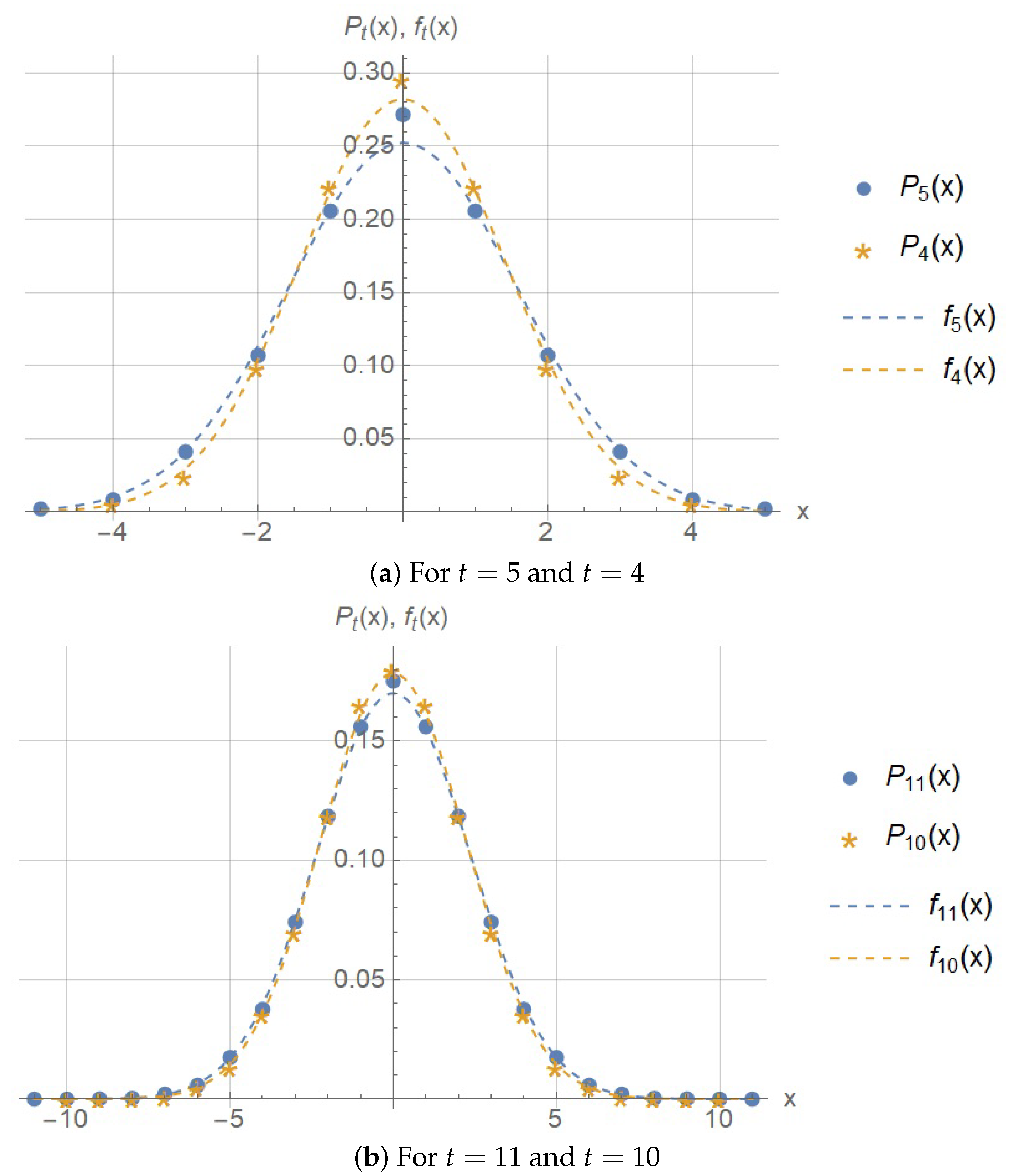
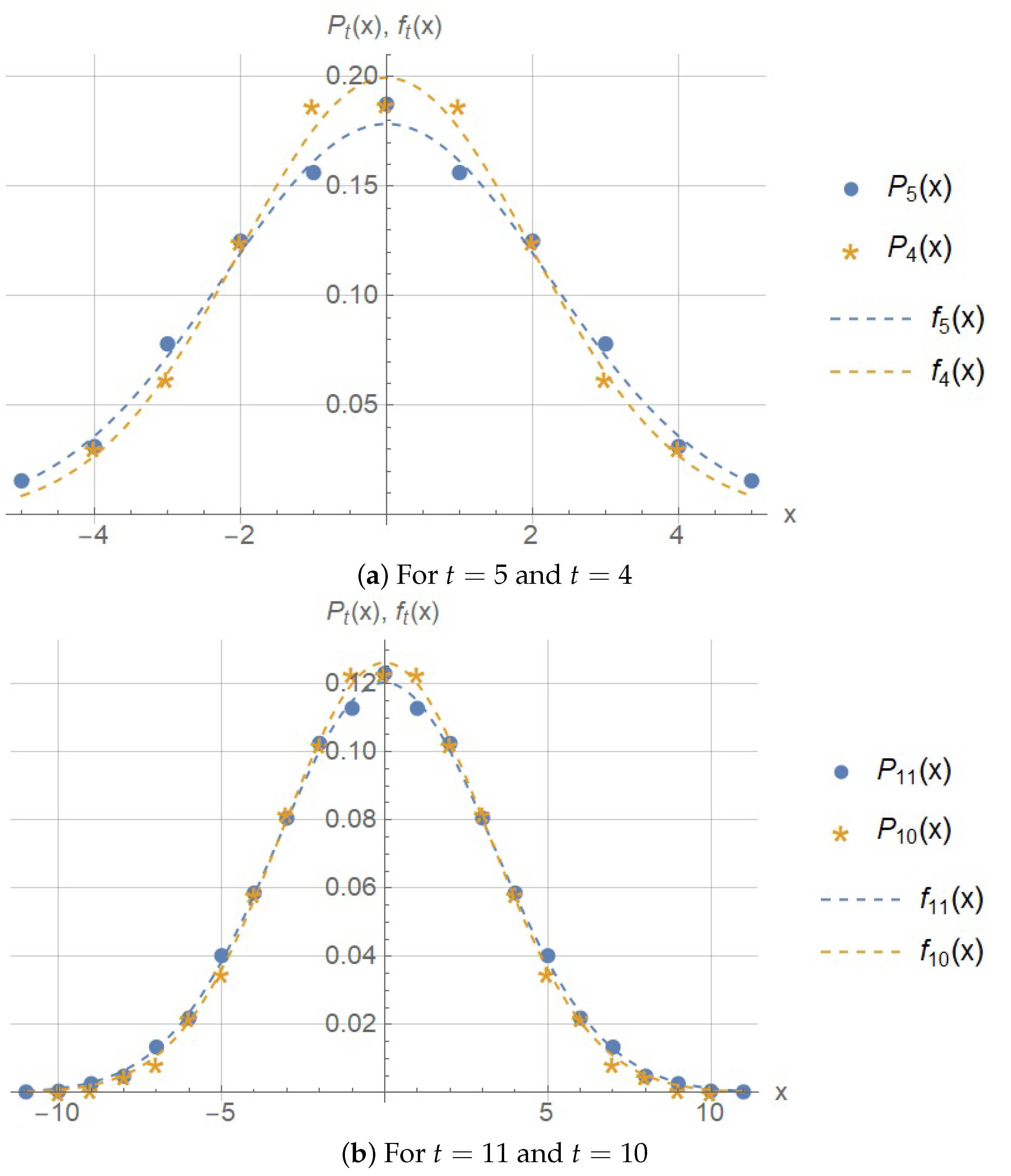
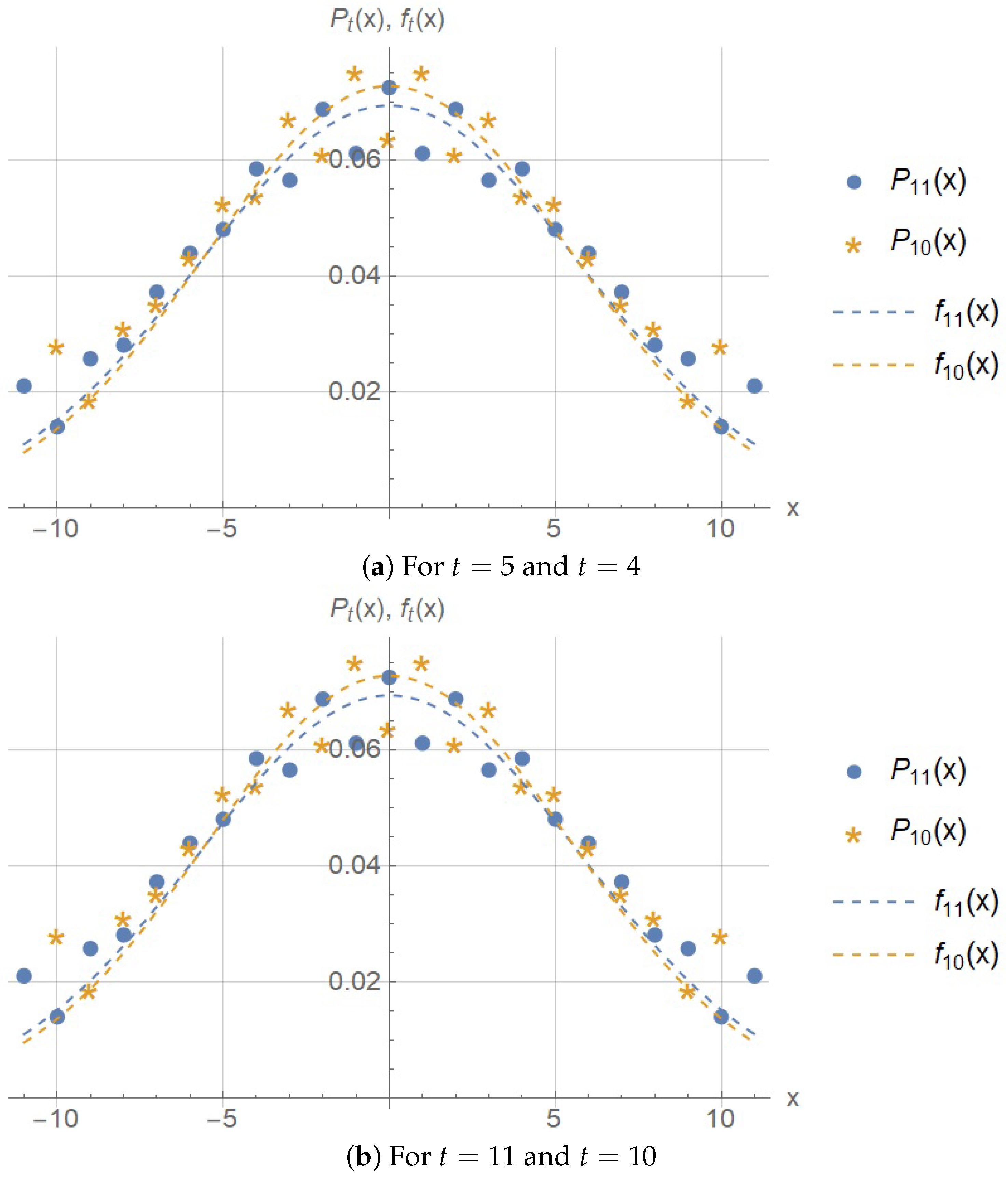
In Figure 3, Figure 4 and Figure 5, the probability distribution from (24)–(27) (or (29) for p = 1 2 ), and (28) is plotted along with the following normal probability distribution:
f t ( x ) = 1 p 2 t π p exp ( 1 p ) x 2 2 t p .
Note that in view of (3), (4) the distribution P t ( x ) tends to f t ( x ) as t at least for p [ 0 ; 1 2 ] . The moments of the normal distribution (31) are given by (30), (23).
From Figure 3 and Figure 4, it is clear that the distribution is very close the normal one even for small t.
Note that the probability p > 1 2 does not make sense for MCA. However, the definition (5) of the two-dimensional Markov chain under consideration admits p ( 0 ; 1 ) ( p = 0 and p = 1 are trivial cases), and Theorem 1 holds for p ( 0 ; 1 ) . For completeness, we have shown the probability distribution for p > 1 2 in Figure 5. Apart from the fact that p > 1 2 has no physical meaning regarding the diffusion, we can note that the probability distribution P t ( x ) is a nonmonotonic function with respect to x 0 for p > 1 2 .
Next, we will discuss the differences between the two types of MCA mentioned in Section 2. Let the MCA parameterized by p be termed the first type MCA. The second type MCA corresponds to the p = 1 2 but it is parameterized by p s . The parameter p s determines the probability that the rotation rule does not applies to any block of the odd and even partition at the next two time steps. In Section 2, we described it as the probability of skipping two consecutive time steps. We will limit ourselves to the simple case when the probability p s is checked only at odd time steps. Note that p s corresponds to the global rule while the probability p corresponds to the local rule since it is checked for each individual block independently.
We have shown that the diffusion coefficient D c ( p ) (30) in the first type MCA nonlinearly depends on p. On the other hand, the diffusion coefficient D c ˜ ( p s ) in the second type MCA linearly depends on p s and is given as follows:
D c ˜ ( p s ) = ( 1 p s ) D c ( 0.5 ) .
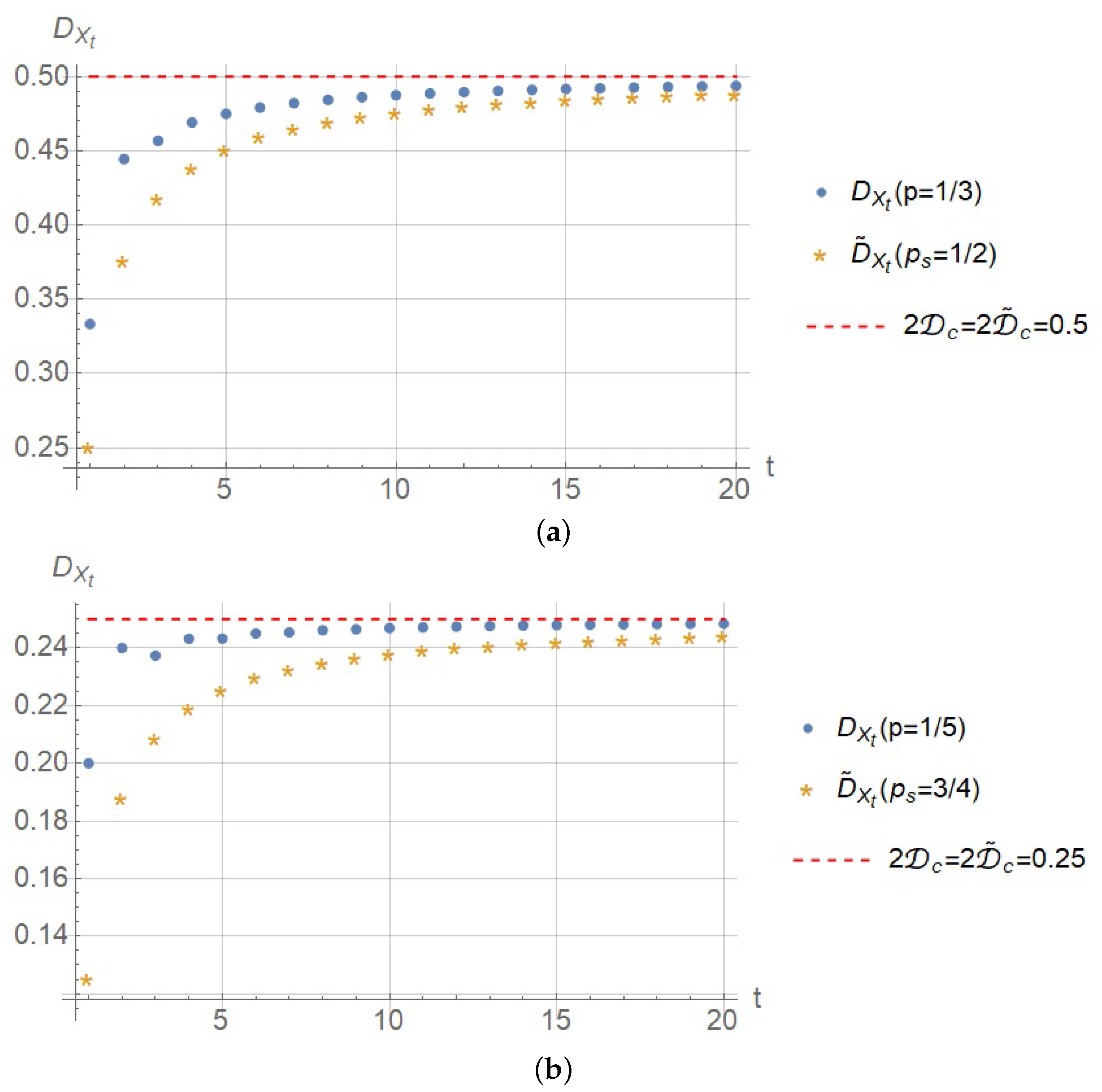
Both of these MCA can be adjusted to the same diffusion coefficient by the appropriate choice of p and p s , i.e., they have the same macroscopic behaviour at large times. However, they behave differently at small times t. Since the first and the third moments of the distribution given by (24)–(28) equal to zero, the core information about the process behaviour is carried by the dispersion. The behaviour of the first type MCA corresponds to the dispersion D X t ( p ) given by (23) while the behaviour of the second type MCA corresponds to the dispersion D ˜ X t ( p s ) given by
D ˜ X t ( p s ) = ( 1 p s ) · D X t ( 0.5 ) .
In Figure 6, the time dependence of D X t ( p ) and D ˜ X t ( p s ) are shown.
We see that the dispersion D X t ( p ) tends to its large time asymptotic value faster than D ˜ X t ( p s ) . Moreover, for small t, it is also much closer to this value that determines the diffusion coefficient in MCA especially for p < 1 2 . It means that the first type MCA shows its macroscopic diffusion behaviour at smaller t. That can be treated as a better time resolution of such MCA. Note that the comparison of the dispersions yields a lower estimate for the time resolution since we do not take into account correlation between the movement of different particles in MCA. However, there is a reason to believe that this correlation is even higher for the second type MCA with p s 1 since the skipping of the two consecutive time steps is performed for the whole cellular grid as opposite to the first type MCA, where it is checked for the every block whether it rotates or not on the current time step. Hence, the difference mentioned above may be even greater than one obtained from our estimates.
Let us compare our analytical results with some empirical results of other authors.
In [20], the author has compared the results of modelling with MCA and solutions of PDE numerically. The diffusion coefficient D c ( 0.5 ) = 0.512 was obtained. The error of 5% was declared in [20]. Their numerical results agrees with the exact value of 0.5 obtained in this work.
In [23], the authors have empirically obtained the dependence of D c ( p ) (in relative units) on p. They constructed the following regression model for this dependence:
p = 0.35 D c ( p ) D c ( 0.5 ) 2 + 0.86 D c ( p ) D c ( 0.5 ) .
Their experimental values for (34) fit well to the curve (30) taking into account the inaccuracy of their method of matching the solutions of MCA and PDE. Hence, they could obtain the regression model that is close to the exact formula if they would use the rational function approximation, which is widely used in many applications [25], instead of the polynomial model.
Note that along with the MCA with the Boolean alphabet the one with the integer alphabet is also used [7,26]. Such approach allows one to lower the concentration noise [27] when modelling reaction–diffusion systems. In order to control the diffusion coefficient independently of reaction rates in such MCA, the rotation rule applies not to the whole integer value but to its percentage. Applying the rotation rule to the percentage of particles is equivalent to the changing the block rotation probability p by the same factor in terms of the diffusion coefficient. Thus, the dependence of the diffusion coefficient on the percentage ξ of particles that are involved in the rotation has the same form as the dependence (30) up to changing ξ = 2 p .
We should note that, in some works related to the multicomponent MCA, reseachers falsely suppose that the dependence D c ( p ) should be linear for a wide range of p. This assumption originates from the work [28], where the authors claimed that D c ( p ) is linear on p even when the rotation probability is independent for each block. Our exact analytical Formula (30) shows that the linear approximation is inaccurate when p is substantially lower than 1 2 . Note that it also agrees with the cited numerical results [23].

7. Conclusions

We have considered the one-parameter stochastic process describing the one-dimensional movement (projection on the x-axis) of a single particle in two-dimensional MCA. In order to find the distribution of the x-coordinate of the particle at every discrete time step (the probability distribution of the random variable X t ), we have introduced the additional random variable Δ t associated with the direction of the movement of the particle. Using our approach, we have reduced this process to the two-dimensional Markov chain of X t and Δ t and have obtained the desired distribution by the probability generating function method. In particular, we have derived the analytic formula for the probability distribution (Theorem 1) and for two first moments (23) of X t . The probability distribution is expressed in compact form in terms of Jacobi polynomials.
The primary results of this work are the Theorem 1 and Formula (30). The Formula (30) gives the diffusion coefficient of the one-parameter two-dimensional MCA. It establishes the correspondence between the cellular automaton model of the diffusion and the kinetic theory. Note that in our formalist diffusion coefficient is given by the asymptotic behaviour of the dispersion of X t for the distribution under consideration. It is shown that the Formula (30) agrees with earlier empirical results of other authors in the specified cases. Since the diffusion rate of real substances is usually given by their diffusion coefficient, the Formula (30) is an important mathematical result for modelling the diffusion using MCA. Theorem 1 gives the probability distribution of a single particle in MCA that is given by the exact solutions to the two-dimensional Markov chain (7), (8), while (30) is of main applied interest, Theorem 1 is a more general fundamental result. It allows us to study specific features of various realizations of MCA discussed in Section 6. Moreover, the exactly solvable two-dimensional Markov chain are also valuable for the fundamental mathematics. In view of Theorem 1, the empirically proven fact that MCA describes the diffusion can be presented as a specific property of Jacobi polynomials (see Figure 3 and Figure 4).
Due to the potential interest of Theorem 1 for other applications, it is worth studying other properties of the process under consideration. Note that the formulae derived in this work are valid for the range p ( 0 ; 1 ) while only p ( 0 ; 1 2 ) have a physical meaning in MCA. Therefore, the more detailed study of this process for the parameter p ( 1 2 ; 1 ) is planned in a separate future work. Furthermore, it is of interest to generalize our approach for the three-dimensional MCA, especially the Formula (30).

Author Contributions

Conceptualization, A.E.K. and A.V.S.; methodology, A.E.K. and A.V.S.; validation, A.E.K. and A.V.S.; formal analysis, A.E.K. and A.V.S.; investigation, A.E.K. and A.V.S.; writing—original draft preparation, A.E.K. and A.V.S.; writing—review and editing, A.E.K. and A.V.S.; visualization, A.E.K. All authors have read and agreed to the published version of the manuscript.

Funding

This research received no external funding.

Institutional Review Board Statement

Not applicable.

Informed Consent Statement

Not applicable.

Data Availability Statement

Not applicable.

Acknowledgments

We are thankful to M.L. Gromov and N.A. Shalyapina for stimulating discussions.

Conflicts of Interest

The authors declare no conflict of interest.

Appendix A. Proof of Theorem 1

Let us write the probability generating function (18) as
G t + ( z , t ) = 1 2 t + 1 m ( z ) [ λ q ( z ) + m ( z ) t 1 q ( z ) m ( z ) t 1 + + 2 ( 1 p + p z ) q ( z ) + m ( z ) t q ( z ) m ( z ) t ] , G t ( z , t ) = 1 2 t + 1 m ( z ) [ q ( z ) + m ( z ) t + 1 q ( z ) m ( z ) t + 1 + + 2 ( 1 p p z ) q ( z ) + m ( z ) t q ( z ) m ( z ) t ] ,
where q ( z ) = p z + 1 z , λ = 4 ( 2 p 1 ) , and m ( z ) is defined in (17). Next, we use the following properties:
q + m t + q m t = 2 k = 0 n C 2 n 2 k q 2 k m 2 n 2 k , t = 2 n , 2 k = 0 n C 2 n + 1 2 k + 1 q 2 k + 1 m 2 n 2 k , t = 2 n + 1 , q + m t q m t m = 2 k = 0 n 1 C 2 n 2 k + 1 q 2 k + 1 m 2 n 2 k 2 , t = 2 n , 2 k = 0 n C 2 n + 1 2 k q 2 k m 2 n 2 k , t = 2 n + 1 ,
and arrive at the following formulae:
G 2 n + 1 + ( z ) = 1 2 2 n + 1 { λ j = 0 n 1 q ( z ) 2 ( n j ) 1 m ( z ) 2 j C 2 n 2 j + 1 + + 2 ( 1 p + p z ) j = 0 n q ( z ) 2 ( n j ) m ( z ) 2 j C 2 n + 1 2 j + 1 } , G 2 n + ( z ) = 1 2 2 n { λ j = 0 n 1 q ( z ) 2 j m ( z ) 2 ( n 1 j ) C 2 n 1 2 j + + 2 ( 1 p + p z ) j = 0 n 1 q ( z ) 2 j + 1 m ( z ) 2 ( n j ) 2 C 2 n 2 j + 1 } , G 2 n + 1 ( z ) = 1 2 2 n + 1 { j = 0 n q ( z ) 2 ( n j ) + 1 m ( z ) 2 j C 2 n + 2 2 j + 1 + + 2 ( 1 p p z ) j = 0 n q ( z ) 2 ( n j ) m ( z ) 2 j C 2 n + 1 2 j + 1 } , G 2 n ( z ) = 1 2 2 n { j = 0 n q ( z ) 2 j m ( z ) 2 ( n j ) C 2 n + 1 2 j + + 2 ( 1 p p z ) j = 0 n 1 q ( z ) 2 j + 1 m ( z ) 2 ( n j ) 2 C 2 n 2 j + 1 } .
Using the relation m 2 ( z ) = q 2 ( z ) λ , the binomial theorem, and changing the order of summation, we transform (A3) to the power series in q ( z ) :
G 2 n + 1 + ( z ) = 1 2 2 n + 1 { k = 0 n 1 q ( z ) 2 ( n k ) 1 ( 1 ) k + 1 λ k + 1 R ( n 1 , k ) + + 2 ( 1 p + p z ) k = 0 n q ( z ) 2 ( n k ) ( 1 ) k λ k Q ( n , k ) } , G 2 n + ( z ) = 1 2 2 n { k = 0 n 1 q ( z ) 2 ( n k 1 ) ( 1 ) k + 1 λ k + 1 Q ( n 1 , k ) + + 2 ( 1 p + p z ) k = 0 n 1 q ( z ) 2 ( n k ) 1 ( 1 ) k λ k R ( n 1 , k ) } , G 2 n + 1 ( z ) = 1 2 2 n + 1 { k = 0 n q ( z ) 2 ( n k ) + 1 ( 1 ) k λ k R ( n , k ) + + 2 ( 1 p p z ) k = 0 n q ( z ) 2 ( n k ) ( 1 ) k λ k Q ( n , k ) } , G 2 n ( z ) = 1 2 2 n { k = 0 n q ( z ) 2 ( n k ) ( 1 ) k λ k Q ( n , k ) + + 2 ( 1 p p z ) k = 0 n 1 q ( z ) 2 ( n k ) 1 ( 1 ) k λ k R ( n 1 , k ) } ,
where the numbers Q, R are given by
R ( n , k ) = j = 0 n k C 2 n + 2 2 j + 1 C n j k , Q ( n , k ) = j = 0 n k C 2 n + 1 2 j C n j k , R ( n , 1 ) = Q ( n , 1 ) 0 .
Using the binomial theorem for the power of q ( z ) , changing the order of summation, in view of (13), we obtain the following identities:
G 2 n + 1 ( z ) = 1 2 2 n + 2 { j = 0 n l = j n p 2 l + 1 a n , l C 2 l + 1 l j z 2 j + 1 + + j = n 1 1 l = j 1 n p 2 l + 1 a n , l C 2 l + 1 l j z 2 j + 1 + + 4 ( 1 p ) j = n n l = | j | n p 2 l b n , l C 2 l l j z 2 j } , G 2 n ( z ) = 1 2 2 n + 1 { j = n n l = | j | n p 2 l r n , l C 2 l l j z 2 j + + 4 ( 1 p ) j = 0 n 1 l = j n 1 p 2 l + 1 d n 1 , l C 2 l + 1 l j z 2 j + 1 + + 4 ( 1 p ) j = n 1 l = j 1 n 1 p 2 l + 1 d n 1 , l C 2 l + 1 l j z 2 j + 1 } ,
where
a n , l = ( 1 ) n l λ n l R ( n 1 , n 1 l ) + R ( n , n l ) , b n , l = ( 1 ) n l λ n l Q ( n , n l ) , r n , l = ( 1 ) n l λ n l Q ( n 1 , n 1 l ) + Q ( n , n l ) , d n , l = ( 1 ) n l λ n l R ( n , n l ) .
In view of (11), we have
P 2 n ( 2 j ) = 1 2 2 n + 1 l = j n p 2 l r n , l C 2 l l j , j = 0 , n ¯ ; P 2 n ( 2 j + 1 ) = 1 p 2 2 n 1 l = j n 1 p 2 l + 1 d n 1 , l C 2 l + 1 l j , j = 0 , n 1 ¯ ; P 2 n + 1 ( 2 j ) = 1 p 2 2 n l = j n p 2 l b n , l C 2 l l j , j = 0 , n ¯ ; P 2 n + 1 ( 2 j + 1 ) = 1 2 2 n + 2 l = j n p 2 l + 1 a n , l C 2 l + 1 l j , j = 0 , n ¯ .
In order to simplify (A8), let us prove the lemma below.
Lemma A1. 
The following relation holds true:
j = 0 n k C 2 n + 1 2 j C n j k = 2 2 ( n k ) C 2 n k k .
Proof. 
Let us define
T ( n , k , j ) = C 2 n + 2 2 j + 1 C n j k = ( 2 n + 1 ) ! ( 2 j ) ! ( 2 n 2 j + 1 ) ! ( n j ) ! k ! ( n j k ) ! .
Using the relation [29]
( 2 n ) ! = 1 2 n ¯ = 4 n 1 2 n ¯ 1 j ¯ ,
where x n ¯ is the Pochhammer function (upper factorial), one readily gets
T ( n , k , j ) = ( 1 ) j n 1 2 j ¯ n ! 1 2 j ¯ j ! k ! ( n j k ) ! .
Then, we have
Q ( n , k ) = j = 0 n k T ( n , k , j ) = C n k · 2 F 1 k n , n 1 2 , 1 2 , 1 .
Here, we have used the formula
j = 0 n C n k ( 1 ) j a j ¯ b j ¯ z n = 2 F 1 n , a , b , z ,
where 2 F 1 m , a , b , z is the hypergeometric function [30,31].
The Gauss summation theorem yields
2 F 1 k n , n 1 2 , 1 2 , 1 = Γ 1 2 Γ 1 + 2 n k Γ 1 2 + n k Γ 1 + n = 2 2 ( n k ) ( 2 n k ) ! ( n k ) ! ( 2 n 2 k ) ! n ! ,
where Γ [ x ] is the gamma function. Then, (A13) and (A15) yield (A9). □
Corollary A1. 
The numbers Q ( n , k ) and R ( n , k ) given by (A5) can be generalized to the functions of a half-integer n that are related as follows:
R ( n , k ) = Q ( n + 1 2 , k ) .
Proof. 
From (A5) and Lemma A1, we have
Q ( n , k ) = 2 2 ( n k ) C 2 n k k .
In a similar way, one can derive the formula
R ( n , k ) = 2 2 ( n k ) + 1 C 2 n k + 1 k ,
Assuming n to be a half-integer number, one readily gets (A16) from (A17) and (A18). □
Let us consider P 2 n + 1 ( 2 j ) from (A8). In view of (A9), (A16), and (A7), substituting l = n k , we obtain
P 2 n + 1 ( 2 j ) = ( 1 p ) p 2 j ( 1 2 p ) j n k = 0 n j ( 1 ) k p 2 2 p 1 k ( n + k + j ) ! k ! ( 2 j + k ) ! ( n j k ) ! .
Using (A14), we arrive at
P 2 n + 1 ( 2 j ) = ( 1 p ) p 2 j ( 1 2 p ) n j C j + n 2 j · 2 F 1 j n , 1 + j + n , 1 + 2 j , p 2 2 p 1 , j = 0 , n ¯ .
In a similar way, one readily gets
P 2 n ( 2 j ) = 1 2 p 2 j ( 1 2 p ) n j ( C j + n 2 j · 2 F 1 j n , 1 + j + n , 1 + 2 j , p 2 2 p 1 + + C n + j 1 2 j · 2 F 1 j n + 1 , j + n , 1 + 2 j , p 2 2 p 1 ) , j = 0 , n 1 ¯ ; P 2 n ( 2 j + 1 ) = ( 1 p ) p 2 j + 1 ( 1 2 p ) n j 1 C j + n 2 j + 1 × × 2 F 1 j n + 1 , 1 + j + n , 2 + 2 j , p 2 2 p 1 , j = 0 , n 1 ¯ ; P 2 n + 1 ( 2 j + 1 ) = 1 2 p 2 j + 1 ( 1 2 p ) n j × × ( C j + n 2 j + 1 · 2 F 1 j n + 1 , 1 + j + n , 2 + 2 j , p 2 2 p 1 + + C j + n + 1 2 j + 1 · 2 F 1 j n , 2 + j + n , 2 + 2 j , p 2 2 p 1 ) , j = 0 , n 1 ¯ .
Finally, using the identities [32]
P n ( α , β ) ( z ) = ( α + 1 ) n ¯ n ! · 2 F 1 n , 1 + α + β + n , α + 1 , 1 2 ( 1 z ) , n + 1 2 α + 1 n + 1 ( 1 + x ) P n ( α , 1 ) ( x ) = P n + 1 ( α , 0 ) ( x ) + P n ( α , 0 ) ( x ) ,
we arrive at the formulae (24), (25), (26), (27).
The probability P n ( n ) (28) can be readily obtained if one notice that the special case X t = t for the given t > 0 is equivalent to Δ t = + 1 t N .
For p = 1 2 , (18) and (13) yield
G t ( z ) = 2 t 1 z + 2 + z k = 0 t 1 C t 1 k s 2 k t + 1 , t N .
From (A23) and (11), we have (29).

References

  1. Wolfram, S. A New Kind of Science; Wolfram Media: Champaign, IL, USA, 2002. [Google Scholar]
  2. Palchaudhuri, A.; Anand, D.; Dhar, A. FPGA fabric conscious architecture design and automation of speed-area efficient Margolus neighborhood based cellular automata with variegated scan path insertion. J. Parallel Distrib. Comput. 2022, 167, 50–63. [Google Scholar] [CrossRef]
  3. Cicuttin, A.; De Micco, L.; Crespo, M.; Antonelli, M.; Garcia, L.; Florian, W. Physical implementation of asynchronous cellular automata networks: Mathematical models and preliminary experimental results. Nonlinear Dyn. 2021, 105, 2431–2452. [Google Scholar] [CrossRef]
  4. Cagigas-Muñiz, D.; Diaz-del Rio, F.; Sevillano-Ramos, J.; Guisado-Lizar, J.L. Efficient simulation execution of cellular automata on GPU. Simul. Model. Pract. Theory 2022, 118, 102519. [Google Scholar] [CrossRef]
  5. Matolygin, A.; Shalyapina, N.; Gromov, M.; Torgaev, S. Tensor approach to software implementation of cellular automata model of diffusion. J. Phys.: Conf. Ser. 2020, 1680, 012035. [Google Scholar] [CrossRef]
  6. Toffoli, T.; Margolus, N. Cellular Automata Machines: A New Environment for Modeling; MIT Press: Cambridge, MA, USA, 1987; p. 276. [Google Scholar]
  7. Kireeva, A.; Sabelfeld, K.K.; Kireev, S. Synchronous multi-particle cellular automaton model of diffusion with self-annihilation. In Parallel Computing Technologies; Lecture Notes in Computer Science (Including Subseries Lecture Notes in Artificial Intelligence and Lecture Notes in Bioinformatics); Springer: Cham, Switzerland, 2019; Volume 11657, pp. 345–359. [Google Scholar] [CrossRef]
  8. Fick, A. On liquid diffusion. J Membr Sci. J. Membr. Sci. 1995, 100, 33–38. [Google Scholar] [CrossRef]
  9. Paul, A.; Laurila, T.; Vuorinen, V.; Divinski, S. Fick’s Laws of Diffusion. In Thermodynamics, Diffusion and the Kirkendall Effect in Solids; Springer: Cham, Switzerland, 2014; pp. 115–139. [Google Scholar] [CrossRef]
  10. Shapovalov, A.; Kulagin, A. Semiclassical approach to the nonlocal kinetic model of metal vapor active media. Mathematics 2021, 9, 2995. [Google Scholar] [CrossRef]
  11. Shapovalov, A.; Kulagin, A.; Siniukov, S. Family of Asymptotic Solutions to the Two-Dimensional Kinetic Equation with a Nonlocal Cubic Nonlinearity. Symmetry 2022, 14, 577. [Google Scholar] [CrossRef]
  12. Odintsov, S. Editorial for Feature Papers 2021–2022. Symmetry 2022, 15, 32. [Google Scholar] [CrossRef]
  13. Mickens, R. Nonstandard finite difference schemes for reaction--diffusion equations having linear advection. Numer. Methods Partial Differ. Equations 2000, 16, 361–364. [Google Scholar] [CrossRef]
  14. Pankov, P.; Zheentaeva, Z.; Shirinov, T. Asymptotic reduction of solution space dimension for dynamic systems. TWMS J. Pure Appl. Math. 2021, 12, 243–253. [Google Scholar]
  15. Shokri, A. The multistep multiderivative methods for the numerical solution of first order initial value problems. TWMS J. Pure Appl. Math. 2016, 7, 88–97. [Google Scholar]
  16. Rachinskaya, M.; Fedotkin, M. Research of a multidimensional Markov Chain as a model for the class of queueing systems controlled by a threshold priority algorithm. Reliab. Theory Appl. 2018, 13, 47–58. [Google Scholar]
  17. Ching, W.K.; Fung, E.S.; Ng, M.K. Higher-order Markov chain models for categorical data sequences. Nav. Res. Logist. 2004, 51, 557–574. [Google Scholar] [CrossRef]
  18. Morzfeldi, M.; Tong, X.T.; Marzouk, Y.M. Localization for MCMC: Sampling high-dimensional posterior distributions with local structure. J. Comput. Phys. 2019, 380, 1–28. [Google Scholar] [CrossRef] [Green Version]
  19. Ching, W.K.; Ng, M.K.; Fung, E.S. Higher-order multivariate Markov chains and their applications. Linear Algebra Its Appl. 2008, 428, 492–507. [Google Scholar] [CrossRef] [Green Version]
  20. Bandman, O.L. Comparative study of cellular-automata diffusion models. Parallel Comput. Technol. 1999, 1662, 395–409. [Google Scholar] [CrossRef]
  21. Malinetskii, G.G.; Stepantsov, M.E. Modeling of diffusion processes by cellular automata with Margolus neighborhood. Comput. Math. Math. Phys. 1998, 38, 973–975. [Google Scholar]
  22. Bandman, O.L. Invariants of cellular automata models for reaction-diffusion processes. Appl. Discret. Math. 2012, 3, 108–120. (In Russian) [Google Scholar] [CrossRef]
  23. Shalyapina, N.; Gromov, M.; Matolygin, A.; Torgaev, S. Empirical dependence of the probability of blocks rotations on the diffusion coefficient in a cellular automaton with a Margolus neighbourhood. J. Phys.: Conf. Ser. 2021, 2140, 012031. [Google Scholar] [CrossRef]
  24. Nelson, R. Probability, Stochastic Processes, and Queueing Theory; Springer: New York, NY, USA, 1995. [Google Scholar] [CrossRef]
  25. Gluzman, S. Padé and Post-Padé Approximations for Critical Phenomena. Symmetry 2020, 12, 1600. [Google Scholar] [CrossRef]
  26. Medvedev, Y. Multi-particle cellular-automata models for diffusion simulation. In Methods and Tools of Parallel Programming Multicomputers; Lecture Notes in Computer Science; Springer: Berlin/Heidelberg, Germany, 2010; Volume 6083, pp. 204–211. [Google Scholar] [CrossRef]
  27. Bandman, O.L. Computation properties of spatial dynamics simulation by probabilistic cellular automata. Future Gener. Comput. Syst. 2005, 21, 633–643. [Google Scholar] [CrossRef]
  28. Chopard, B.; Frachebourg, L.; Droz, M. Multiparticle lattice gas automata for reaction diffusion systems. Int. J. Mod. Phys. C 1994, 5, 47–63. [Google Scholar] [CrossRef]
  29. Bateman, H.; Erdélyi, A. Higher Transcendental Functions; McGraw-Hill: New York, NY, USA, 1953; Volume 1. [Google Scholar]
  30. Srivastava, H.M. A Survey of Some Recent Developments on Higher Transcendental Functions of Analytic Number Theory and Applied Mathematics. Symmetry 2021, 13, 2294. [Google Scholar] [CrossRef]
  31. Srivastava, H.M. Some Families of Generating Functions Associated with Orthogonal Polynomials and Other Higher Transcendental Functions. Mathematics 2022, 10, 3730. [Google Scholar] [CrossRef]
  32. Bateman, H.; Erdélyi, A. Higher Transcendental Functions; McGraw-Hill: New York, NY, USA, 1953; Volume 2. [Google Scholar]
Figure 1. Odd and even partitions of the cell grid. Solid lines divide the cell grid into blocks of the odd partition and dashed lines divide the cell grid into blocks of the even partition. Arrows demonstrate the rotation rule.
Mathematics 11 00584 g001
Figure 2. Examples of possible movements of a particle in the MCA. The black dot is for the particle movement at an odd time step (the rotation rule applies for blocks of the odd partition) and the white dot is for the particle movement at an even time step (the rotation rule applies for block of the even partition).
Mathematics 11 00584 g002
Figure 3. The plot of the probability distribution P t ( x ) along with the plot of the normal probability distribution function f t ( x ) for p = 1 3 .
Mathematics 11 00584 g003
Figure 4. The plot of the probability distribution P t ( x ) along with the plot of the normal probability distribution f t ( x ) for p = 1 2 .
Mathematics 11 00584 g004
Figure 5. The plot of the probability distribution P t ( x ) along with the plot of the normal probability distribution f t ( x ) for p = 3 4 .
Mathematics 11 00584 g005
Figure 6. The time plot of the dispersion of the X t for two types of the MCA. It illustrates the macroscopic behaviour of these MCA at small times. The parameters in (a) correspond to MCA with the diffusion coefficient of 0.25 , and the parameters in (b) correspond to MCA with the diffusion coefficient of 0.125 .
Mathematics 11 00584 g006
Disclaimer/Publisher’s Note: The statements, opinions and data contained in all publications are solely those of the individual author(s) and contributor(s) and not of MDPI and/or the editor(s). MDPI and/or the editor(s) disclaim responsibility for any injury to people or property resulting from any ideas, methods, instructions or products referred to in the content.