Abstract
In this study, a cogeneration cycle in a time-transient state is investigated and optimized. A quasi-equilibrium state is assumed because of the small time increments. Air temperature and solar power are calculated hourly. The cycle is considered in terms of energy, exergy, and economic and environmental analyses. Increasing the net present value (the difference between the present value of the cash inflows and outflows over a period of time) and reducing exergy destruction are selected as two optimization objective functions. The net present value is calculated for the period of 20 years of operation according to the operation parameters. The optimization variables are selected in such a way that one important variable is selected from each system. To optimize the cycle, the particle swarm optimization method is used. The number of particles used in this method is calculated using the trial-and-error method. This cycle is optimized using 13 particles and 42 iterations. After optimization, the energy efficiency increased by 0.5%, the exergy efficiency increased by 0.25%, and the exergy destruction decreased by 1% compared to the cycle with existing parameters.
Keywords:
optimization; cogeneration of water and electricity; time-transient analysis; sensitivity analysis; solar power MSC:
80M50
1. Introduction
Solar energy is one of the most important renewable resources that is available to humanity without pollution in most parts of the world. In addition, water is one of the important elements of human life. Therefore, the cogeneration of electricity and freshwater using solar energy has been the subject of research by many researchers. Most thermal power plants are combined-cycle power plants (CCPP), gas turbines [1], heat recovery steam generators (HRSG), and steam turbines (ST) [2]; by optimizing the amount of fuel consumption and heat loss in the condenser, the cycles can be optimized in terms of energy consumption. There are various ways to increase the overall efficiency of the cycles and to reduce environmental costs. The use of solar energy and the generation of freshwater using the dissipated heat of the condenser are examples of these solutions. Therefore, using such solutions is one of the ways to develop combined CCPPs. Energy-exergy-economic-environmental (4E) analysis and the optimization of different combinations of these cycles have been the subject of research by many researchers.
A solar-powered CO2 Brayton cycle with an MED (multi-effect distillation) system for the cogeneration of water and electricity was Combined by Kouta et al. [3,4] in 2017.
Two systems are considered in this study. The first system is integrating a solar tower with a regeneration sCO2 cycle and an MEE-TVC (multi-effect evaporation with thermal vapor compression) desalination system, and the second system is integrating a solar tower with a recompression sCO2 cycle and an MEE-TVC desalination system. The MED system has a steam compression system with a TVC thermal compressor. The energy consumption of the system is equal to 3 KW to generate each m3 of fresh water.
The combination of an MED water desalination system with a gas power plant was investigated in 2019 [5]. In this study, the cogeneration cycle in the city of San Diego, which includes a power plant with a capacity of 115 MW with an efficiency of 48% as well as an MED system with a generation capacity of 1558 m3 per day of fresh water (1.81 $/m3) to the title of the reference cycle, was considered, and after modeling the performance, the system was investigated for different locations. The obtained results show that, among all the investigated cases, the country of Saudi Arabia has the lowest cost for the cogeneration of water and electricity.
The feasibility for the introduction of decentralized combined heat and power plants in agricultural processes was performed by Dimitris et al. [6] in 2022. Critical parameters for the project’s economic viability in this article are the electricity selling price from the CCPP unit (higher than 0.12 €/kWh) and the biogas procurement price (lower than 0.046 €/kWh).
The dynamic modeling of a combined concentrating solar tower and parabolic trough for increased day-to-day performance was investigated by Georgios et al. [7]. This system achieved a higher maximum capacity factor of 18% at 925 W/m2 at a cost of electricity of 248 Euro/MWh.
The combined operation of a wind-pumped hydro storage plant with a concentrating solar power plant for insular systems was studied by Georgios et al. [8]. The price of electricity in this system was reported in the range of 0.20 EUR/kWh.
A combined system of a steam turbine power plant and an MED system using a linear solar system was investigated in 2017 [9]. Both LF/SRC and PTC/SRC plants were considered to generate a specific electricity rate (107.5 MWh), while the condenser of the plants was replaced by an MED desalination unit to produce fresh water (100,000 m3/day). They also considered a boiler unit with natural gas for situations when the required solar energy is not available.
A multi-objective optimization on a cogeneration system consisting of a combined cycle power plant and an MSF (multi-stage flash) desalination unit was performed in 2012 [10]. The new environmental costing function was merged in the thermo-economic objective, and a new thermo-environomic function was obtained. By applying the genetic algorithm, this objective function was minimized, whereas the system exergy efficiency was maximized.
In 2010, the time-dependent optimal operation of an RO (reverse osmosis) desalination system was investigated by Ghobeti and Mitsos [11]. In this research, the time period of half an hour was considered, and by reducing the time period of the analysis, it was investigated as a steady state. In another study in 2012, a solar heat power receiver and storage system using a salt bath concentrated solar power on demand (CSPonD) in terms of design and operation was optimized [12]. Solar energy is used to generate steam for a steam turbine. The optimization of the design for the CSPonD shows that the virtual two-tank conceptual design considered does not result in significantly lower salt requirements compared to single-tank thermal energy storage.
The time-dependent operation of solar thermal power plants for the cogeneration of power and freshwater was investigated [13] in 2011. In this research, different combinations of thermal power plants with different methods of seawater desalination were investigated, and the use of objective functions was continuous in the optimization process. This power plant is a combination of a solar power concentrator in a salt bath, Rankine cycle, RO, and an MED desalination system. The results show that, for the plant size considered (4 MWe equivalent nominal capacity) and the MED design chosen based on the literature and industry practice, RO is preferred over MED from an energy point of view. In addition, under the current feed-in tariff (FiT) and water prices in Cyprus, extracting steam for MED is not recommended.
The analysis of different seawater hybrid desalination systems in combination with different power and water cogeneration methods was investigated in 2013 [14]. In this research, different combinations of water desalination methods with thermal power generation methods were investigated in terms of energy and economy.
The optimal design and operation of different desalination systems were studied in 2014 [15]. In this research, the old methods were examined first. Then, the application of these methods using new energies [16] was suggested.
The multi-objective optimization of a solar hybrid cogeneration cycle using a genetic algorithm in the Matlab optimization toolbox to reduce carbon emissions was studied by Soltani et al. [17] in 2014. In this article, eight decision variables (such as rc, TIT, etc.) were chosen to optimize the fuel consumption, CO2 emission, and exergy destruction. The technical results of the optimum decision variables were a 48% reduction in fuel consumption, which consequently avoids 24.5 tons of CO2 annual emissions, and a considerable decrease in chemical exergy destruction as the main source of irreversibility.
The technical and economic feasibility of integrating CSP technologies with cogeneration gas turbine systems were investigated in 2017 to produce electricity and steam [18]. Three CSP technologies (solar towers, parabolic trough collectors, and linear Fresnel reflectors) were assessed for possible integration with a gas turbine cogeneration system that generates steam throughout the year in addition to the generation of electricity. Several simulations for hourly, daily, and annually averaged performances for all sizes of gas turbine cogeneration plants were investigated. For a gas turbine size of 70 MWe, the three CSP technologies have comparable annual solar shares. Several simulations were studied using THERMOFLEX with the PEACE software.
A new cogeneration system including a high-temperature proton exchange membrane fuel cell integrated with a solar methanol steam reformer and a Kalina cycle was proposed to produce electricity and heat [19]. Detailed thermal modeling was performed to simulate the parabolic trough collector along with its associated storage tank performance. The decision variables were chosen to optimize the exergy efficiency, total product unit cost, and carbon dioxide (CO2) emission factor. The optimization results show that the average daily exergy efficiency can increase by up to 29.3%, and the total product unit cost as well as the carbon dioxide mass specific emission can decrease by up to 17.72% and 16.3%, respectively, compared to the corresponding values under the base conditions.
An innovative hybrid solar/biomass cogeneration plant was designed and optimized to generate power and heat [20] in 2021. The proposed system includes PV/T (photovoltaic/thermal), a PEM (proton exchange membrane), a biomass gasifier, a GT cycle, an SRC (steam Rankine cycle), and TEG (thermoelectric generator) components. Two multi-objective optimizations based on the NSGAII (non-dominated sorting genetic algorithm) were employed to achieve the best design point for the exergy efficiency and the total cost rate of the system and also the exergy efficiency and LCOE (levelized cost of electricity) of the system. The energy and exergy efficiencies of this system were determined as 69.15% and 23.11%, respectively. This system produces 14.55 MW of electricity with a total cost rate of 633.04 $/h and a unit product cost of 4.66 $/GJ.
The optimal integration of a linear Fresnel reflector with a gas turbine cogeneration power plant was investigated in 2017 [21]. The main objective of the present work is to investigate the possible modifications of an existing gas turbine cogeneration plant, which has a gas turbine of 150 Mwe electricity generation capacity and produces steam at a rate of 81.4 kg/s at 394 °C and 45.88 bars, for an industrial process.
The time-transient analysis of solar thermal power plants with heat storage was investigated and optimized by Garcia et al. [22]. The solar thermal power storage system in this research is of the concentrated solar power on demand type in the salt bath (CSPonD).
The annual thermo-economic time-transient analysis of a cycle for the cogeneration of power and freshwater was investigated in 2020 [23]. This cycle is a combination of a steam generation solar cycle for a steam turbine with an MED system and a photovoltaic solar power plant to supply the required electricity for the sea water transfer pump to the heights. This cycle was analyzed using the TRNSYS software. Under the moderately fluctuating electricity price, the use of heaters increases the revenue significantly compared to the same case with no electric heaters considered. In the case of a highly fluctuating electricity price, the use of heaters more than doubles the revenue.
The 4E analysis and the exergetic and economic optimization of a cycle for the cogeneration of water and electricity using fossil fuels and solar power were investigated by Ghasemiasl et al. and Javadi et al. [24,25]. This cycle is a combination of a CCPP with an MED system, which uses solar energy to steam in the HP steam turbine section. The power plant optimization results show that the exergy efficiency increases to 53.62%, which indicates a growth of 1.74%. The efficiency of the plant after applying a lithium-bromide refrigeration cycle and a solar collector increased from 50.33 to 51.73%, while the exergy efficiency was enhanced from 47.48 to 48.22%. In addition, it was concluded that adding a collector and absorption chiller led to a 1.5% reduction in environmental pollutants.
Ghasemiasl et al. [26], in a study in 2021 to reduce the environmental effects caused by a CCPP, converted this cycle into a cogeneration cycle of electricity, fresh water, and hydrogen and presented the 4E analysis of this cycle. This cycle is a combination of a CCPP with an ORC, MED, and PEM. The proposed system has an exergy efficiency of 49.64% and an energy efficiency of 57.36%. In addition, by reducing 9.8% of pollutants, this system reduced the production of 27,400 tons of pollutants into the atmosphere per year, and by reducing the fuel consumption, it saved $8.7 million in annual power plant fuel costs.
The energy, exergy, and economic analyses of a new multiple-cogeneration cycle relying on fossil fuels and solar energy were analyzed by Javadi et al. [27]. This cycle is able to cogenerate power, hydrogen, heat, and cold. The multi-generation system has an energy and exergy efficiency of 19% and 19.29%, respectively, and the costs of electricity and H2 production are equal to 0.1477 $/kWh and 7.626 $/kg.
Different methods for the generation of electricity using different solar methods were examined in 2018 [28]. PV-based systems are more suitable for small-scale power generation.
The thermodynamic analysis and multi-objective optimization of a CCPP along with an ORC cycle were performed in 2018 [29]. The exergo-economic analysis showed that the combustion chamber had the highest sum of exergy destruction costs and investment costs. Under the design conditions, an exergy efficiency of 40.75% and a product cost rate of 439 million $/year could be achieved.
Therefore, according to the articles mentioned in the above literature review, the time-transient optimization of the cogeneration of electricity and freshwater using a combination of CCPPs, solar panels, and heat-receiving towers at the inlet of HRSGs, ORCs, RO, and MEDs has not been studied yet. Therefore, according to the cases mentioned in the history of the above research, the stress analysis has not yet been investigated, and its investigation can be an attractive topic for researchers in the field of energy.
In this research, first, the system is modeled according to the hourly air temperature of the study area throughout the year, and the whole system is analyzed in terms of energy, exergy, economic balance, and environmental effects. Due to the short period of time, the time variations in energy, exergy, and mass are insignificant, and their gradient is neglected with respect to time. The amount of exergy destruction and the NPV (net present value) of this design are calculated for 20 years of operation, and it is optimized by maximizing the NPV and minimizing the exergy destruction of the cycle. The design variables are selected in such a way that one effective parameter is selected from each part. The differences in articles similar to this article are given in Table 1.

Table 1.
The differences in articles similar to this article.
In summary, the novelty and advantages of this study are:
- ✓
- The increase in system efficiency by using solar energy instead of HRSG burners;
- ✓
- The increase in system efficiency by using the waste energy of the outlet vapor from steam turbines;
- ✓
- The sensitivity analysis to produce sustainable fresh water throughout the year;
- ✓
- The production of power and freshwater simultaneously by designing this multi-generation system;
- ✓
- The use of power generated by ORC for use in RO desalination pumps;
- ✓
- The optimization of system energy and exergy efficiency by proposing some methods that reduce the exergy destruction of the components;
- ✓
- The optimization of the NPV of the cogeneration system;
- ✓
- The cycle simulation was conducted transiently with time and cycle optimization as a transient optimization with time.
2. System Description
The scheme of the studied system consists of a CCPP, solar system, ORC, MED, and RO, and the connections between all the sub-systems are shown in Figure 1.
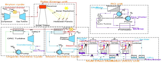
Figure 1.
Schematic of the GT, HRSG, ST, ORC, RO, and MED systems for the generation of electricity and fresh water using fossil fuels and solar energy.
The outlet hot-air temperature of the gas turbine is almost constant and must be increased to enter the triple-pressure HRSG (two water vapor pressures and one organic fluid pressure). As depicted in Figure 1, the solar system consists of a heliostat panel and a solar receiver tower, which increases the outlet air temperature of the gas turbine as a variable of time with a specified maximum value due to the number of panels and solar radiation variation at all hours of the day during the year. This maximum value is determined according to the design limitations of the HRSG. The exhaust air from the heat receiver tower passes through the inlet burners of the HRSG, and the burners increase the inlet air temperature to the HRSG up to the specified maximum value and fix the temperature by consuming fuel that varies with time. The hot air, which passes through the HRSG, produces high-pressure and medium-pressure water vapor for the steam turbine and low-pressure organic steam for the ORC. The outlet steam pressure of the steam turbine increases to the saturation pressure at 70 °C to enter the MED system so that all the outlet steam of the steam turbine enters the MED system and exchanges heat with the seawater entering the MED system. The main purpose of this system is the cogeneration of energy and water in an optimized state. Hypotheses have been used to model this cycle:
- (1)
- The inlet air temperature to the compressor is variable on an hourly basis;
- (2)
- The isentropic efficiency of the Brayton cycle is just considered a temperature function;
- (3)
- The fuel used in the Brayton cycle and boiler burners is methane with a fixed LHV;
- (4)
- The turbines and all components are considered with zero depreciation conditions;
- (5)
- It is assumed that the gas turbine, steam turbine, and all components operate at all times with their nominal load;
- (6)
- The air outlet temperature from the HRSG exhaust has a limit of at least 125 °C due to the area’s high humidity;
- (7)
- The steam turbine outlet enters the MED system fully instead of entering the condenser;
- (8)
- The HRSG has a pinch and approach temperature of 9 °C for producing water vapor;
- (9)
- The HRSG has three pressures, the low pressure of which is related to the organic cycle.
3. Mathematical Modelling
3.1. 4E Analysis of the Cycle of Cogeneration of Electricity and Fresh Water
The 4E analysis includes energy, exergy, economic, and environmental analyses to calculate the first law efficiency, fuel consumption, net power generation, net freshwater generation, second law efficiency, exergy destruction rate, electricity generation cost rate per kilowatt-hour (Kwh), freshwater generation cost rate per m3, and the environmental effects caused by the carbon production.
In order to analyze the time-transient energy, the one-year time period is divided into hourly time periods, and the law of conservation of mass and the first law of thermodynamics are solved for each hourly time period. Due to the fact that the time intervals are small enough, the time gradient of mass and energy can be ignored, and as a result, the energy analysis relations are expressed as Equations (1) and (2).
In energy analysis, due to the fact that the inlet air conditions are considered hourly and time-variable, all conditions and parameters are calculated hourly and as time-variable. By choosing a time interval small enough, the accuracy of the solution is increased.
Exergy is a characteristic of a system that expresses the ability of that system to do work. The exergy of a system is divided into two parts, including thermodynamic exergy and chemical exergy. The thermodynamic exergy is divided into three parts, including physical, kinetic, and potential, where the kinetic and potential exergy can be ignored versus the physical exergy. The specific exergy of a system is calculated from Equation (3).
The exergy balance relation for each control volume is calculated from Equation (4) from which the amount of exergy destruction () is calculated.
Exergeoeconomics is a branch of engineering that was created from the combination of thermodynamics and economics. In an exergeoeconomic analysis, the cost balance for each component of the system is written in the form of Equation (5) [21].
In Equation (5), represents the inlet exergy cost, represents the outlet exergy cost, represents the initial investment cost rate of operation and maintenance for each subsystem, represents the cost of the net electricity consumption, and represents the fuel consumption cost rate where is the fuel consumption cost, and is the mass flow rate of fuel consumption. The relations to calculate the cost rate of each subsystem are obtained from Equation (6) [30].
In Equation (6), represents the number of years of operation, which is usually considered 20 years, represents the interest rate, which is usually considered 0.15%, represents the number of operation hours for each subsystem in a year, represents the repair and maintenance coefficient for each piece of equipment, which is usually considered 1.06, and represents the initial cost of each subsystem, which can be calculated experimentally for each piece of equipment.
3.2. Optimization of the Cogeneration of Water and Electricity Cycle
In the PSO algorithm, similar to any other optimization algorithm, particles are first randomly distributed in the problem-solving space. It should be noted that the problem-solving space is an n-dimensional space where n is the number of design variables for which optimal values are supposed to be found.
For each particle that is moving in the solution space of the problem, two important and basic variables are defined, which include position and speed. The initial position of all particles in the group is randomly determined, and their initial velocity is also considered equal to zero. With the start of the optimization process, the particles start moving in the problem-solving space so that at each stage of the optimization, the velocity vector of each particle (which is actually the displacement vector of that particle, but in this method, it is known as the velocity vector) is determined according to two main factors as follows:
- The best position that the particle has experienced since the beginning of the optimization process until that moment (intrinsic intelligence of the particle);
- The best position experienced by one of the particles belonging to the group from the beginning of the optimization process until that moment (collective wisdom of the group).
Suppose we want to find the optimal point for the function so that is a column vector; as mentioned earlier, n is the number of design variables for which the optimal values are to be determined. In summary, this minimization problem can be defined as follows:
In Equation (7), and represent the lower limit and the upper limit of the vector , respectively.
The PSO algorithm is performed by following the steps below:
- Consider the number of particles (usually 20 to 30 particles are enough [31]);
- At the initial moment (), distribute the particles () randomly in the solution space, and calculate the value of the objective function () for all particles;
- Consider the initial speed of all particles to be zero, and consider the iteration counter as ;
- In the iteration for the particle, determine the following two variables:
- d.1
- The best position that this particle has had in all previous iterations ();
- d.2
- The best position that one of the particles belonging to the group has had until that moment ().
Using these two variables, calculate the velocity vector (displacement vector) for the particle in the iteration as follows:
In Equation (8), and are random numbers in the range [0, 1], and and are coefficients between 1 and 2 that show the importance of intrinsic intelligence and collective wisdom, respectively [31].
In Equation (9), the coefficient is called an inertia term, and its value decreases linearly from to in the successive stages of optimization as follows:
The reason for the reduction in this coefficient during the optimization process is that, with the passage of time, the particles will be closer to the optimal point, and it is better to move around this point at a slower speed so as not to pass through it. Usually, values of and are more useful [31].
Now, using the Equation (10), the position of the j-th particle is calculated in the i-th iteration as follows:
The value of the objective function () is calculated again for all particles.
- e.
- If the swarm is gathered at the same point (convergence desired by the designer is satisfied), is the optimal answer, and if the convergence desired by the designer is not satisfied, , and step 4 must be repeated.
In Equation (11), m is the number of constraints. One of the ways to satisfy the constraints in constrained optimization problems is a method called the penalty function method. In this method, the constraints determined for the problem are added to the objective function, and their value will vary during the optimization steps depending on whether the constraint is satisfied or not. Liu and Lin [32] suggested that the objective function be defined as follows:
where
Equations (12) and (13) show that if a condition is satisfied (), it is removed from the objective function, and if it is not satisfied, its value is added to the objective function in the form of a penalty function.
In Equation (12), the variable is known as the error variable, which is calculated as follows [32]:
where , , , .
4. Analysis of the Results
In this section, the optimization of the cycle is carried out by using the particle swarm intelligent meta-initiative optimization (PSO) algorithm. The goal is to increase, as much as possible, the NPV of the cycle and to reduce the exergy destruction, and therefore, the objective function is defined as to be minimized.
A CCPP for the cogeneration of electricity and fresh water, which generates the electricity and freshwater with an initial cost of construction and with the cost of operation and maintenance during the period of operation, which is about 20 years, and the cost of fossil fuel consumption, the NPV variable is calculated for the entire operation period.
This variable includes initial costs, consumption costs, operation and maintenance costs, and sales rates of products, and at the same time, includes the efficiency first and second laws of thermodynamics and economic and environmental factors.
This variable is a function of time and the current interest rate, and according to the current interest rate, it calculates the real value of the system for the 20-year period of operation and the system’s implementation period.
Considering the simplicity and dependence of this variable on economic factors, interest rate, and operation and maintenance cost coefficients, by calculating this variable in each design, the profit or loss of that design can be determined. The positivity of this variable indicates the profitability of the design, and its negativity indicates the loss of the design. Therefore, as this variable becomes larger for a design, the profitability of that design will be larger.
Therefore, by maximizing the NPV function, which is a function of the cycle design parameters, the optimal state of the cycle can be determined. The NPV relation is expressed as Equation (15) [33].
In Equation (15), is the time of operation, is the interest rate, is the net cash flow at time t, and N is the total time of implementation, operation, and maintenance. In this research, the interest rate is 15%, the implementation time is 2 years, the operation time is 20 years, the adjustment rate is 12%, and the inflation rate is 10%.
Exergy destruction has also been explained in previous sections, and it is a destructive factor; by reducing it, the ability of a system to do work increases, and as a result, the efficiency of a system approaches its maximum efficiency. Therefore, by minimizing this variable, the system will be optimized.
All the selectable variables that play a role in the calculation of the objective function and can be selected for optimization are given in Table 2.
Table 2.
Important variables in the calculation of the objective function.
The design variables for optimizing the objective function of the cycle were selected in such a way that, for each cycle, a variable that has the most significant effect on it, was selected and can be easily changed in each part.
For the gas cycle, the flow rate of the inlet air was chosen because the flow rate of the inlet air is effective in all parts and can be adjusted, but the compression ratio of the compressor and the temperature of the inlet air to the gas turbine is an inherent characteristic of the turbine itself.
In the solar system, the maximum temperature of the outlet air from the heat receiving tower and entering the recovery boiler, which determines the total number of mirrors and, total surface area of the mirrors, and the variable fuel consumption of the burners, was selected. In fact, this variable is common between the recovery boiler and the solar system. By increasing this temperature, the number of mirrors and the fuel consumption will increase, and as a result, the initial investment cost and operation cost will increase. The efficiency of the cycle will decrease, but it will be possible to generate more steam for the steam Rankine cycle and the organic Rankine cycle.
For the steam Rankine cycle (SRC), three variables, the flow rate of the inlet steam to the HP and LP turbines and the pressure of the outlet steam from the ST, were selected because the decrease or increase in each of these three variables will have a significant effect on the generation capacity of the steam Rankine cycle and will also have a significant effect on the performance of the MED system and ORC.
For the ORC, the pressure of the inlet organic steam to the turbine was selected, which has a significant effect on the generation power in this cycle.
For the MED system, the number of effects was selected, which has a significant effect on the flow rate of the generated freshwater in the MED system.
For the RO system, the generation rate of freshwater was selected. By increasing it, the pump power, initial cost, and operation cost increase, and in return, the freshwater generation and the income from the freshwater’s sale also increase.
Therefore, the design variables are eight variables in the form of the flow rate of the inlet air to the gas turbine, the temperature of the inlet air to the recovery boiler, the flow rate of the generated steam to the HP turbine, the flow rate of the generated steam to the MP turbine, the pressure of the ORC steam, the pressure of the outlet steam of the steam turbine, the number of MED effects, and the flow rate of the generated freshwater in RO are defined as a column vector with eight elements in the form of Equation (16).
In this regard, the concept of each of the variables and their variations are presented in Table 3.
Table 3.
Physical concept of the variables and their variations.
The constraints given in Table 2 were selected based on the design limitations and using the trial-and-error method. For example, if the number of effects is less than 4, the MED system will not be able to start, or if the flow rate of the generated steam to the HP turbine is more than 70 kg/s, the recovery boiler will not be able to generate organic steam for the ORC.
In order to prevent each of the design variables from leaving the specified range during the optimization process, 16 constraints were defined as follows:
In the modeling section of the system, three constraints were defined inside the model, and these constraints were implemented in the modeling and were not implemented in the optimization process. First, the number of mirrors and their arrangement were selected based on the maximum temperature of inlet air to the recovery boiler. Second, the decrease in the temperature of the outlet air of the recovery boiler due to the air humidity by the seaside has a maximum value of 110 degrees Celsius. With this constraint, the flow rate of the organic steam generated in the recovery boiler for the organic Rankine cycle turbine was limited. Thirdly, the entire flow rate of the outlet steam from the steam turbine entered the MED system with the limitation that the pressure of the outlet steam increased until it was ready to start the MED system.
One of the challenges of the optimization method with the PSO method was the number of selected particles. By choosing different numbers of particles, different optimal solutions were given, and the particles preferred different optimal solutions, and some of these optimal points were relative optimal points. The number of iterations in each of the particles continued until all the particles accumulated at the optimal point, which was usually about 40 iterations for each of the numbers of particles.
In this research, first, for the number of different particles, the graph of the objective function value is depicted as a function of the number of particles in order to determine the number of particles that gives the optimal point using the trial-and-error method. The graph of the objective function value as a function of the number of particles is given in Figure 2.
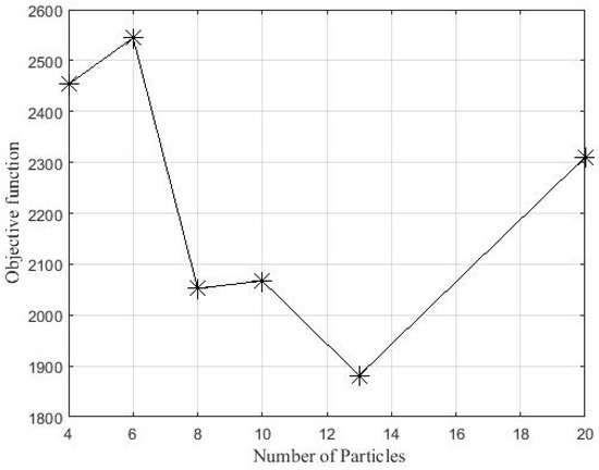
Figure 2.
Objective function diagram for different numbers of particles.
As can be seen from Figure 2, the minimum value of the objective function is obtained when the number of particles is 13. Therefore, in this research, the number of particles was chosen equal to 13.
The optimization process was conducted by selecting 13 particles and implementing 42 iterations ( and ). It should be mentioned that the number of particles and the number of iterations were obtained by the trial-and-error method, and with this number of particles and iterations, the answers of the variables converged.
Due to a large number of iterations, the results of the position of the particles in the first state and multiple iterations of five until the final accumulation of particles are shown in Figure 3.
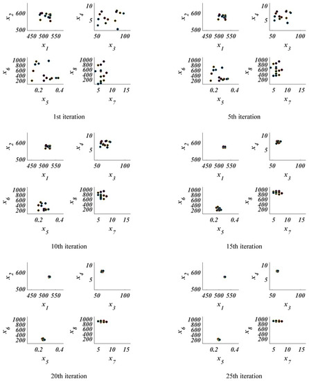
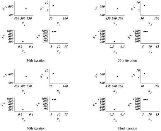
Figure 3.
The movement of particles during the optimization process of the solar power plant with and .
As Figure 3 shows, the particles accumulated in the 42nd iteration in the eight-dimensional problem-solving space. In this optimal situation, the values of each of the design variables are as follows:
The value of the objective function at this optimal point is .
The energy efficiency increased by 0.5%, the exergy efficiency increased by 0.25%, and the exergy destruction decreased by 1% compared to the cycle with existing parameters.
5. Validation
As this system is a new one and the combination of its subsystems does not exist in any past studies, to validate the equations obtained, each subsystem can be validated with available data in past studies. The GT and Rankine cycle were validated with the results of the Shirkoh Yazd CCPP plant and are given and compared in Table 4. The CCPP plant was validated with reference [26] and is compared in Table 5. The results of the ORC (for R141b organic fluid) were validated with reference [26] in Table 6.
Table 4.
Results of the gas turbine and Rankine cycle validation.
Table 5.
Validation results for CCPP.
Table 6.
Validation results for ORC (for R141b organic fluid).
The results of the MED desalination are compared with reference [34] in Table 7. The results of the RO desalination for producing 145.8 m3/h of freshwater were compared with reference [35] and are given in Table 8. The results of the SPT (solar power tower) are compared with reference [36,37,38] in Table 9.
Table 7.
Validation results for the MED system.
Table 8.
Validation results for the RO system.
Table 9.
Validation results for the SPT cycle.
As is illustrated in these tables, the maximum difference is 3% due to the simplifying assumptions that were considered to solve the equations, and the results of solving the equations in this article are in good agreement with past research.
Usually, in optimization methods, the relative optimal point is obtained. Therefore, the optimal point obtained is not the absolute optimal point. In optimization, the variables should be determined so that the objective function is optimized according to the constraints. To prove that the optimal point has been calculated, the change graph of the objective function was drawn with respect to each of the variables and compared with the location of the optimal point. For example, all the variables except the mass flow rate of the incoming air were kept constant and the graph of changes in the objective function with respect to the mass flow rate of the incoming air is given in Figure 4. In the same way, the graph of changes in the objective function was drawn for each of the variables, and these graphs are shown in Figure 4, Figure 5, Figure 6, Figure 7, Figure 8, Figure 9, Figure 10 and Figure 11. After checking these graphs, as can be seen, the optimal point in all the graphs is in the minimum state with respect to the objective function.
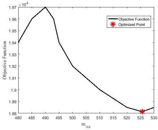
Figure 4.
Variations in the objective function with the air flow rate.
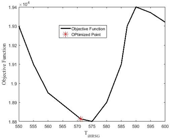
Figure 5.
Variations in the objective function with the TiHRSG.
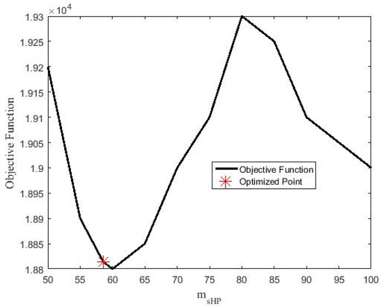
Figure 6.
Variations in the objective function with the steam flow rate of the HP.
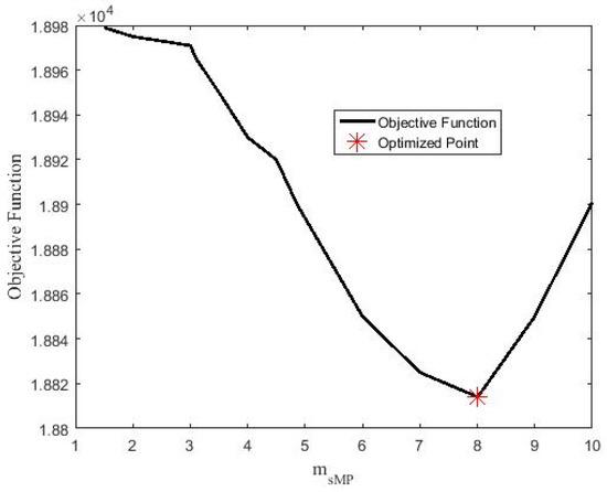
Figure 7.
Variations in the objective function with the steam flow rate of the MP.
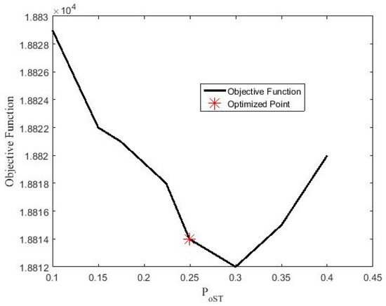
Figure 8.
Variations in the objective function with the output pressure of the ST turbine.
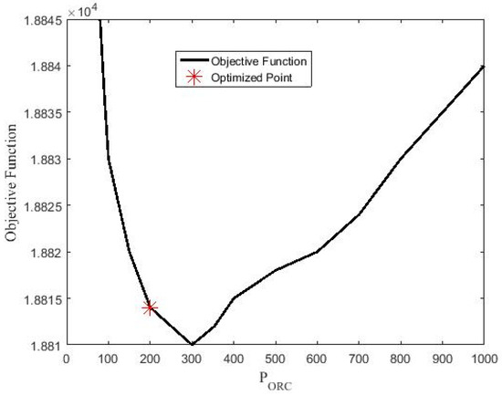
Figure 9.
Variations in the objective function with the input pressure of the ORC turbine.
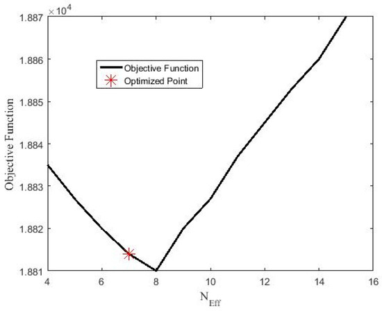
Figure 10.
Variations in the objective function with the number of MED effects.
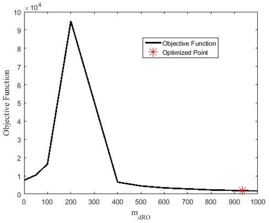
Figure 11.
Variations in the objective function with the desalinated water from RO.
Therefore, it can be concluded that the optimal point obtained in the previous section can be one of the optimal points of this cycle, and the obtained results are correct. It should be noted that this cycle has not been optimized by any of the researchers, and the results of this research cannot be compared with the results of other studies.
6. Conclusions
In this study, a combined cycle for the cogeneration of water and electricity was investigated and optimized. The solar power receiver tower was placed between the recovery boiler and the gas turbine outlet using heliostat panels. The excess heat of the outlet air from the HRSG is used to generate organic steam for the ORC. The entire steam outlet from the steam turbine enters a MED system to generate fresh water. An RO desalination system generates freshwater by consuming electricity from the ORC subsystem. The temperature of the inlet air to the gas turbine varies with time and changes hourly. This system was analyzed in terms of energy, exergy, and economy, and then, the results of the analysis were used to optimize the cycle for operation for 20 years. This design was analyzed and optimized for the weather conditions of Bandar Abbas, one of the cities along the Persian Gulf. By properly choosing the parameters of the flow rate of the inlet air, the temperature of the inlet air to the recovery boiler, the flow rate of the inlet steam to the steam turbine, the pressure of the outlet steam from the steam turbine, the pressure of the ORC vapor, the number of MED effects, and the consumption of the RO power, an optimal state of the system was designed. The outlet steam pressure of the steam turbine is an important design parameter; by increasing it, the final efficiency of the cycle can be increased to an acceptable level. By increasing the pressure of the outlet steam from the steam turbine, the steam required by the MED system is supplied, and with a slight decrease in the net generation power, the amount of generated freshwater increases. By reducing the flow rate of the generated steam for the steam turbine, it is possible to generate steam with a better quality and, in return, generate a greater flow rate of organic steam for the ORC. Reducing the temperature of the inlet air to the recovery boiler reduces fuel consumption and the cost of the initial investment in the solar panels, but on the other hand, the effect of the ORC is reduced. Therefore, there is a suitable optimum temperature for the temperature of the inlet air to the HRSG. The energy efficiency increased by 0.5%, the exergy efficiency increased by 0.25%, and the exergy destruction decreased by 1% compared to the cycle with existing parameters.
Author Contributions
Conceptualization, M.A.J. and R.G.; methodology, K.H.; software, K.H.; validation, K.H. and M.A.J.; writing—original draft preparation, K.H.; writing—review and editing, M.A.J.; supervision, R.G. and M.M.d. All authors have read and agreed to the published version of the manuscript.
Funding
This research received no external funding.
Data Availability Statement
The data is unavailable due to privacy.
Conflicts of Interest
The authors declare no conflict of interest.
Abbreviations
| Acronym | |
| CCPP | Combined cycle power plant |
| CSPonD | Concentrated solar power on demand |
| GT | Gas turbine |
| HP | High tressure |
| HRSG | Heat recovery steam generator |
| LP | Low pressure |
| LHV | Lower heating value kJ/kg |
| MED | Multi-effect distillation |
| MSF | Multi-stage flash |
| MEE-TVC | Multi-effect vvaporation with thermal vapor compression |
| NPV | Net present value |
| RO | Reverse osmosis |
| TIT | Turbine inlet temperature |
| PSO | Particle swarm optimization |
| Symbols | |
| A | Area (m2) |
| Membrane area (m2) | |
| Cost per unit of exergy ($/kJ) | |
| Cost of exergy destruction ($/h) | |
| Specific heat (kJ/kg.°C) | |
| Distillated water | |
| Exergy flow rate (kW) | |
| Exergy destruction flow rate (kW) | |
| Mass flow rate kg/s | |
| s | Specific entropy (kJ/kg-K) |
| h | Specific enthalpy (kJ/kg) |
| Power (kW) | |
| T | Temperature (K, or C) |
| Mass flow rate (kg/s) | |
| I | Annual interest rate (%) |
| n | Number of effects |
| Number of heliostats | |
| P | Pressure (kPa) |
| Heat transfer rate (kW) | |
| R | Gas constant (kJ/kg-K) |
| Compressor pressure ratio | |
| The cost of purchasing each component ($) | |
| Investment cost rate ($/h) | |
| Mass flow rate kg/s |
References
- Wang, Y.; Shi, Y.; Luo, Y.; Cai, N.; Wang, Y. Dynamic analysis of a micro CHP system based on flame fuel cells. Energy Convers. Manag. 2018, 163, 268–277. [Google Scholar] [CrossRef]
- Kongtragool, B.; Wongwises, S. A review of solar-powered Stirling engines and low temperature differential Stirling engines. Renew. Sustain. Energy Rev. 2003, 7, 131–154. [Google Scholar] [CrossRef]
- Kouta, A.; Al-Sulaiman, F.; Atif, M.; Marshad, S.B. Entropy, exergy, and cost analyses of solar driven cogeneration systems using supercritical CO2 Brayton cycles and MEE-TVC desalination system. Energy Convers. Manag. 2016, 115, 253–264. [Google Scholar] [CrossRef]
- Kouta, A.; Al-Sulaiman, F.A.; Atif, M. Energy analysis of a solar driven cogeneration system using supercritical CO2 power cycle and MEE-TVC desalination system. Energy 2017, 119, 996–1009. [Google Scholar] [CrossRef]
- Sharan, P.; Neises, T.; McTigue, J.D.; Turchi, C.J.D. Cogeneration using multi-effect distillation and a solar-powered supercritical carbon dioxide Brayton cycle. Desalination 2019, 459, 20–33. [Google Scholar] [CrossRef]
- Katsaprakakis, D.A.; Moschovos, T.; Michopoulos, A.; Kargas, I.D.; Flabouri, O.; Zidianakis, G. Feasibility for the introduction of decentralised combined heat and power plants in agricultural processes. A case study for the heating of algae cultivation ponds. Sustain. Energy Technol. Assess. 2022, 53, 102757. [Google Scholar] [CrossRef]
- Arnaoutakis, G.E.; Katsaprakakis, D.A.; Christakis, D.G. Dynamic modeling of combined concentrating solar tower and parabolic trough for increased day-to-day performance. Appl. Energy 2022, 323, 119450. [Google Scholar] [CrossRef]
- Arnaoutakis, G.E.; Kefala, G.; Dakanali, E.; Katsaprakakis, D.A. Combined Operation of Wind-Pumped Hydro Storage Plant with a Concentrating Solar Power Plant for Insular Systems: A Case Study for the Island of Rhodes. Energies 2022, 15, 6822. [Google Scholar] [CrossRef]
- Askari, I.B.; Ameri, M.J.D. The application of linear Fresnel and parabolic trough solar fields as thermal source to produce electricity and fresh water. Desalination 2017, 415, 90–103. [Google Scholar] [CrossRef]
- Hosseini, S.R.; Amidpour, M.; Shakib, S.E.J.D. Cost optimization of a combined power and water desalination plant with exergetic, environment and reliability consideration. Desalination 2012, 285, 123–130. [Google Scholar] [CrossRef]
- Ghobeity, A.; Mitsos, A. Optimal time-dependent operation of seawater reverse osmosis. Desalination 2010, 263, 76–88. [Google Scholar] [CrossRef]
- Ghobeity, A.; Mitsos, A. Optimal design and operation of a solar energy receiver and storage. J. Sol. Energy Eng. 2012, 134, 031005. [Google Scholar] [CrossRef]
- Ghobeity, A.; Noone, C.J.; Papanicolas, C.N.; Mitsos, A. Optimal time-invariant operation of a power and water cogeneration solar-thermal plant. Sol. Energy 2011, 85, 2295–2320. [Google Scholar] [CrossRef]
- Zak, G.M.; Ghobeity, A.; Sharqawy, M.H.; Mitsos, A. A review of hybrid desalination systems for co-production of power and water: Analyses, methods, and considerations. Desalination Water Treat. 2013, 51, 5381–5401. [Google Scholar] [CrossRef]
- Ghobeity, A.; Mitsos, A. Optimal design and operation of desalination systems: New challenges and recent advances. Curr. Opin. Chem. Eng. 2014, 6, 61–68. [Google Scholar] [CrossRef]
- Rheinländer, J.; Lippke, F.J.R.E. Electricity and potable water from a solar tower power plant. Energy 1998, 14, 23–28. [Google Scholar] [CrossRef]
- Soltani, R.; Keleshtery, P.M.; Vahdati, M.; KhoshgoftarManesh, M.; Rosen, M.; Amidpour, M. Multi-objective optimization of a solar-hybrid cogeneration cycle: Application to CGAM problem. Energy Convers. Manag. 2014, 81, 60–71. [Google Scholar] [CrossRef]
- Mokheimer, E.M.; Dabwan, Y.N.; Habib, M.A. Optimal integration of solar energy with fossil fuel gas turbine cogeneration plants using three different CSP technologies in Saudi Arabia. Appl. Energy 2017, 185, 1268–1280. [Google Scholar] [CrossRef]
- Sarabchi, N.; Mahmoudi, S.S.; Yari, M.; Farzi, A. Exergoeconomic analysis and optimization of a novel hybrid cogeneration system: High-temperature proton exchange membrane fuel cell/Kalina cycle, driven by solar energy. Energy Convers. Manag. 2019, 190, 14–33. [Google Scholar] [CrossRef]
- Teymouri, M.; Sadeghi, S.; Moghimi, M.; Ghandehariun, S. 3E analysis and optimization of an innovative cogeneration system based on biomass gasification and solar photovoltaic thermal plant. Energy 2021, 230, 120646. [Google Scholar] [CrossRef]
- Dabwan, Y.N.; Mokheimer, E.M. Optimal integration of linear Fresnel reflector with gas turbine cogeneration power plant. Energy Convers. Manag. 2017, 148, 830–843. [Google Scholar] [CrossRef]
- Lizarraga-Garcia, E.; Ghobeity, A.; Totten, M.; Mitsos, A. Optimal operation of a solar-thermal power plant with energy storage and electricity buy-back from grid. Energy 2013, 51, 61–70. [Google Scholar] [CrossRef]
- Mata-Torres, C.; Palenzuela, P.; Zurita, A.; Cardemil, J.M.; Alarcón-Padilla, D.-C.; Escobar, R.A. Annual thermoeconomic analysis of a Concentrating Solar Power+ Photovoltaic+ Multi-Effect Distillation plant in northern Chile. Energy Convers. Manag. 2020, 213, 112852. [Google Scholar] [CrossRef]
- Ghasemiasl, R.; Javadi, M.A.; Nezamabadi, M.; Sharifpur, M. Exergetic and economic optimization of a solar-based cogeneration system applicable for desalination and power production. J. Therm. Anal. Calorim. 2021, 145, 993–1003. [Google Scholar] [CrossRef]
- Javadi, M.A.; Ahmadi, M.H.; Khalaji, M. Exergetic, economic, and environmental analyses of combined cooling and power plants with parabolic solar collector. Environ. Prog. Sustain. Energy 2020, 39, e13322. [Google Scholar] [CrossRef]
- Ghasemiasl, R.; Abhari, M.K.; Javadi, M.A.; Ghomashi, H. 4E investigating of a combined power plant and converting it to a multigeneration system to reduce environmental pollutant production and sustainable development. Energy Convers. Manag. 2021, 245, 114468. [Google Scholar] [CrossRef]
- Javadi, M.A.; Abhari, M.K.; Ghasemiasl, R.; Ghomashi, H. Energy, exergy and exergy-economic analysis of a new multigeneration system based on double-flash geothermal power plant and solar power tower. Sustain. Energy Technol. Assess. 2021, 47, 101536. [Google Scholar] [CrossRef]
- Ahmadi, M.H.; Ghazvini, M.; Sadeghzadeh, M.; Alhuyi Nazari, M.; Kumar, R.; Naeimi, A.; Ming, T. Solar power technology for electricity generation: A critical review. Energy Sci. Eng. 2018, 6, 340–361. [Google Scholar] [CrossRef]
- Mohammadi, A.; Ashouri, M.; Ahmadi, M.H.; Bidi, M.; Sadeghzadeh, M.; Ming, T. Thermoeconomic analysis and multiobjective optimization of a combined gas turbine, steam, and organic Rankine cycle. Energy Sci. Eng. 2018, 6, 506–522. [Google Scholar] [CrossRef]
- Khaljani, M.; Saray, R.K.; Bahlouli, K. Comprehensive analysis of energy, exergy and exergo-economic of cogeneration of heat and power in a combined gas turbine and organic Rankine cycle. Energy Convers. Manag. 2015, 97, 154–165. [Google Scholar] [CrossRef]
- Rao, S.S. Engineering Optimization: Theory and Practice; John Wiley & Sons: New York, NY, USA, 2019. [Google Scholar]
- Liu, J.-L.; Lin, J.-H. Evolutionary computation of unconstrained and constrained problems using a novel momentum-type particle swarm optimization. Eng. Optim. 2007, 39, 287–305. [Google Scholar] [CrossRef]
- Bonabeau, E.; Dorigo, M.; Marco, D.d.R.D.F.; Theraulaz, G.; Théraulaz, G. Swarm Intelligence: From Natural to Artificial Systems; Oxford University Press: Oxford, UK, 1999. [Google Scholar]
- Mistry, K.H.; Antar, M.A.; Lienhard V, J.H. An improved model for multiple effect distillation. Desalination Water Treat. 2013, 51, 807–821. [Google Scholar] [CrossRef]
- Nafey, A.; Sharaf, M. Combined solar organic Rankine cycle with reverse osmosis desalination process: Energy, exergy, and cost evaluations. Renew. Energy 2010, 35, 2571–2580. [Google Scholar] [CrossRef]
- Javadi, M.A.; Khodabakhshi, S.; Ghasemiasl, R.; Jabery, R. Sensivity analysis of a multi-generation system based on a gas/hydrogen-fueled gas turbine for producing hydrogen, electricity and freshwater. Energy Convers. Manag. 2022, 252, 115085. [Google Scholar] [CrossRef]
- Ijadi Maghsoodi, A.; Ijadi Maghsoodi, A.; Mosavi, A.; Rabczuk, T.; Zavadskas, E. Renewable Energy Technology Selection Problem Using Integrated H-SWARA-MULTIMOORA Approach. Sustainability 2018, 10, 4481. [Google Scholar] [CrossRef]
- Nabipour, N.; Mosavi, A.; Hajnal, E.; Nadai, L.; Shamshirband, S.; Chau, K.W. Modeling climate change impact on wind power resources using adaptive neuro-fuzzy inference system. Eng. Appl. Comput. Fluid Mech. 2020, 14, 491–506. [Google Scholar] [CrossRef]
Disclaimer/Publisher’s Note: The statements, opinions and data contained in all publications are solely those of the individual author(s) and contributor(s) and not of MDPI and/or the editor(s). MDPI and/or the editor(s) disclaim responsibility for any injury to people or property resulting from any ideas, methods, instructions or products referred to in the content. |
© 2023 by the authors. Licensee MDPI, Basel, Switzerland. This article is an open access article distributed under the terms and conditions of the Creative Commons Attribution (CC BY) license (https://creativecommons.org/licenses/by/4.0/).