Abstract
In the present paper, an algorithm for the numerical solution of the external Dirichlet generalized harmonic problem for a sphere by the method of probabilistic solution (MPS) is given, where “generalized” indicates that a boundary function has a finite number of first kind discontinuity curves. The algorithm consists of the following main stages: (1) the transition from an infinite domain to a finite domain by an inversion; (2) the consideration of a new Dirichlet generalized harmonic problem on the basis of Kelvin’s theorem for the obtained finite domain; (3) the numerical solution of the new problem for the finite domain by the MPS, which in turn is based on a computer simulation of the Weiner process; (4) finding the probabilistic solution of the posed generalized problem at any fixed points of the infinite domain by the solution of the new problem. For illustration, numerical examples are considered and results are presented.
Keywords:
external Dirichlet generalized harmonic problem; probabilistic solution; Wiener process; computer simulation; sphere MSC:
35J05; 35J25; 65C30; 65N75
1. Introduction
It is well known that there are many problems from the various fields of physics (for example, thermostatics, electrostatics, hydrostatics, etc.) that could be considered as external Dirichlet generalized harmonic problems.
First of all, we should note that the requirement of continuity for the boundary function in Dirichlet’s classical harmonic problem is a very strong constraint, because in practical stationary problems (connected with electric, thermal and other static fields), there are cases when it is necessary to discuss and study 2D or 3D Dirichlet generalized harmonic problems. The problems of this type appeared in the literature mainly from the 1940s (see [1,2,3,4,5]).
It is known (see [1,6]) that the methods used to obtain an approximate solution of the classical boundary-value problems are (a) less suitable or (b) not suitable at all for solving generalized boundary value problems. In the first case, the convergence of corresponding approximate process is very slow in neighborhood of boundary singularities and, consequently, the accuracy of approximate solution of the generalized problem is very low (see [1,2,3,4,5]). In the second case, the process is unstable. For example, a similar phenomenon takes place when solving the 3D Dirichlet generalized harmonic problem by the method of fundamental solutions.
In the above-mentioned literature, simplified, or so-called “solvable” generalized problems (the problems “whose” solutions can be constructed by series with terms, represented by special functions), are considered. The methods of the separation of variables, particular solutions, and heuristic methods are mainly applied for their solution, therefore the accuracy of the solution is rather low. Since heuristic methods do not guarantee that the best solution will be found (moreover, in some cases they may give an incorrect solution), it is necessary to check these solutions in order to establish how well they satisfy all the conditions of a problem (see [1]). In addition, it should be noted that, in the literature (see [4] (pp. 346–348)), while solving the Dirichlet external generalized harmonic simplest problem for a sphere, the existence of a discontinuity curve is ignored.
The study of Dirichlet’s generalized 2D and 3D problems in terms of the existence and uniqueness of solution, and selection of a reliable and effective method for its numerical solution has been intensively carried out since the 21st century in the Department of Computational Methods of the Niko Muskhelishvili Institute of Computational Mathematics.
The choice and construction of computational schemes (algorithms) mainly depend on the problem class, dimension, geometry and location of singularities on the boundary. In particular, for solving the Dirichlet generalized plane harmonic problems the following approaches may be used: (I) a method of reduction of Dirichlet generalized harmonic problems to a classical problem (see [7,8]); (II) a method of conformal mapping (see [9]); (III) a method of probabilistic solution (see [10,11]). It is evident that in the case of 3D Dirichlet harmonic problems, from the above mentioned approaches we can apply only third one.
In order to imagine the difficulties associated with the numerical solution of not only generalized, but also the classical external 3D harmonic Dirichlet problem, we will give below a brief overview of several works related to these topics.
In [12], the boundary conditions for the numerical solution of elliptic equations in exterior regions are considered. Such equations in exterior regions frequently require a boundary condition at infinity to ensure the well-posedness of the problem. Practical applications include examples of the Helmholtz and Laplace’s equations. The constructed algorithm requires the replacement of the condition at infinity by a boundary condition on a finite artificial surface. Direct imposition of the condition at infinity along the finite boundary results in large errors. A sequence of boundary conditions is developed which provides increased accuracy of approximations to the problem in the infinite domain. Estimates of the error are obtained for several cases.
In [13], the Laplace–Dirichlet problem is investigated in a three-dimensional case. The Laplace–Dirichlet problem is investigated similarly to the Laplace–Neumann problem, except for the boundary condition. Corresponding variational formulation is considered. It is based on the introduction of an auxiliary unknown by the means of the decomposition of the function u.
In the paper [14], the analytic–numerical method for solving 3D exterior problems for elliptic equations under Dirichlet and Neumann boundary conditions in half-space is considered. Based on analytical transformation, the external boundary problem is reduced to the internal one; then, the corresponding difference problem is considered based on the grid methods [6,7,8]. By using the considered analytic–numerical method for solving external boundary problems in a three-dimensional semispace, the initial problem is reduced to such a problem, the solution of which is possible by traditional techniques and methods of numerical analysis.
In [15], the solution of direct and inverse exterior boundary value problems via the strongly conditioned stochastic method is considered, mainly for exterior harmonic problems. Note that, in numerical examples from the Section 4.2 of [15], experiments were performed with cones of different thickness and observation points in the near and far fields. However, actually, the observation points given in Table 1 of [15] are “not too far” from the field, when we consider the exterior boundary value problems.
It is known that elliptic problems in external domains arise in many branches of physics. For example, the Laplace equation arises in the studies of thermostatic and electrostatic fields external to given surfaces (see [3,16]); the flow of an incompressible irrotational fluid around a body is described by the same equation (see [17]), and so on.
In these cases, infinity can be regarded as a separate boundary. A condition at infinity is required to make the external problem well posed. For the Laplace equation, it is sufficient to impose a condition of regularity at infinity. In the three dimensional (3D) case, the condition is , for , where is the distance from a fixed (but chosen arbitrary) origin (see [18,19]).
2. Statement of the Problem
Let be an infinite domain in the Euclidean space , where is a kernel with a spherical surface (with the center at the point O and the radius R, respectively). Since the harmonicity of a function is invariable under the linear transformation of the Cartesian coordinate system, therefore without loss of generality we assume that the origin of coordinates is at the point .
Let us formulate the following problem.
Problem 1
(A). The function is given on the boundary of the infinite region D and is continuous everywhere, except a finite number of curves , which represent discontinuity curves of the first kind for the function . It is required to find a function satisfying the conditions:
where is the Laplace operator, c is a real constant.
On the basis of Equation (3), in general, the values of are not uniquely defined on the curves (). In particular, if Problem 1 concerns the determination of the thermal (or the electric) field, then we must take when , respectively. In this case, in the physical sense the curves are non-conductors (or dielectrics). Otherwise, will not be a discontinuity curve.
It is evident that surface is divided into the parts by the curves (), where one of the following conditions holds: , , . Thus, the boundary function has the following form
where () are the parts of without discontinuity curves, respectively; the functions , ( are continuous on the parts . It is evident that
Remark 1.
If the domain D is finite with a surface S, then the problem of type A with the conditions (1)–(3) has a unique solution depending continuously on the data (see [20,21]).
It should be noted that the condition (4) is essential for the uniqueness of solution of the Problem 1. Indeed, if out of (4) Problem 1 has any solution , then is its solution as well, where and k is a real constant, i.e., it has an infinite set of solutions.
On the other hand, if Problem 1 has a solution, then it is unique. Assume that Problem 1 with the boundary function (5) has two solutions and , then is a solution of Problem 1 with null boundary value and for function condition (4) is fulfilled. It is known (see [19] p. 303) that, in the noted case when (or , . The existence of solution of the Problem 1 will be shown in Section 3. Based on the above-mentioned, we can investigate by Problem 1 only such physical phenomena, which are damped at infinity.
In the case of external 3D Dirichlet generalized harmonic problems, the difficulties become more significant. In particular, there does not exist a standard algorithm which can be applied to a wide class of domains.
On the basis of noted above, for the numerical solution of the Problem 1 we should apply an algorithm which does not require the approximation of a boundary function and in which the existence of discontinuity curves is not ignored. The method of probabilistic solution (MPS) is one such method (see [20,21]), but its direct application in infinite domains is impossible.
Performed investigations showed (see [10,11,22,23,24,25,26,27]) that the MPS is ideally suited for numerical solution of both classical and generalized (2D and 3D) Dirichlet harmonic problems for a wide class of finite domains only.
Therefore, construction of efficient high accuracy computational schemes for the numerical solution of external 3D Dirichlet generalized harmonic problems (which can be applied to a wide class of domains) has both theoretical and practical importance.
3. Transition from the Infinite Domain to the Kernel by an Inversion and Consideration of a New Problem on the Basis of Kelvin’s Theorem
In the Problem 1 the domain D is infinite, therefore, the direct application of the MPS to its solving is impossible. In order to solve the Problem 1 using MPS, we perform transition from the domain D to the kernel by means of the inversion (see [4,28]). Let a point and consider the following inversions:
with respect to the sphere . The points x and are called symmetric points with respect to the sphere . From Equation (6) (or Equation (7)) we have
It is known (see [4] p. 260) that on the basis of Equation (6) (or Equation (7)) the symmetric points and x with respect to the sphere are situated on the ray, whose beginning is at the point (or ).
It is easy to see that by Equation (8) the infinite domain D is transformed one-to-one onto the . In particular, the points of are transformed into itself, and the point is transformed into the point and vice versa.
On the basis of Equation (7) the functions and are transformed into the functions
respectively, where , , .
It is easy to see that the function is not harmonic in the domain . However, we can remove the noted defect, if we apply Kelvin’s theorem [4,28].
Theorem 1.
If a function is harmonic in the infinite domain D, then the function
is harmonic in the domain .
The function is bounded in the neighborhood of the point , therefore this point for is a removable singular point [4,28]. However, actually, on the basis of the Theorem 1, for extension of harmonicity of function at the point we must solve the following Dirichlet generalized harmonic problem.
Problem 2
(). Find a generalized harmonic function satisfying the conditions:
where in Equation (12): , (), ( and c are the same that in Problem 1.
It is known (see [20,21]) that the generalized problem (11)–(13) is well-posed, i.e., the solution exists, is unique and depends continuously on the data. Respectively, Problem 1 is correct.
It is evident that for solving the Problem 2 we can apply the MPS. In particular, if we want to find the value of the solution of Problem 1 at a point x (), first of all we have to find the image of x by means of (6) and then find the solution of the Problem 2 at the point .
Finally, on the basis of Equation (10) we have
where .
4. The Method of Probabilistic Solution and Simulation of the Wiener Process
In this section we describe the solution of Problem 2 by the MPS. It is known (see [21,24]) that the probabilistic solution of Problem 2 at the fixed point has the following form
In Equation (15) is the mathematical expectation of values of the boundary function at the random intersection points of the trajectory of the Wiener process and the boundary ; is a random moment of the first exit of the Wiener process from the domain . It is assumed that the starting point of the Wiener process is always , where the value of desired function is being determined. If the number N of the random intersection points () is sufficiently large, then according to the law of large numbers, from (15) we have
or for , in probability. Thus, if we have the Wiener process, the approximate value of the probabilistic solution to the Problem 2 at point is calculated by the formula (16).
In order to simulate the Wiener process we use the following recursion relations (see [20,24]):
according to which the coordinates of point are being determined. In Equation (17) are three normally distributed independent random numbers for the k-th step, with zero means and variances equal to one (The above numbers are generated apart); is the number of quantification such that and when , then the discrete process approaches the continuous Wiener process. In the implementation, random process is simulated at each step of the walk and continues until its trajectory crosses the boundary.
In the considered case computations are performed and the random numbers are generated using MATLAB function randn which generates normally distributed random numbers.
Remark 2.
In general, problems of type A can be solved by the MPS for all such locations of discontinuity curves, which give the possibility to establish the part of surface S where the intersection point is located.
5. Numerical Examples
It should be noted that in the 3D case there are no test solutions for generalized problems of type 2, therefore, for the verification of the scheme needed for the numerical solution of Problem 2, the reliability of obtained results can be demonstrated in the following way.
If in boundary conditions (12) of Problem 2 we take , where (), , and denotes the distance between points and , then it is evident that the curves () represent removable discontinuity curves for the boundary function . Actually, in the mentioned case instead of generalized Problem 2 we obtain the following Dirichlet classical harmonic problem.
Problem 3
(B). Find a Function satisfying the conditions:
We solve this problem (by the MPS) using the program used for the Problem 2. It is well-known that the Problem 3 is well posed, i.e., its solution exists, is unique and depends on data continuously. Evidently, an exact solution of the Problem 3 is
Note that application of the MPS for numerical solution of the Dirichlet classical harmonic problems is interesting and important (see [10,11,22,23]). In this paper, the Problem 3 has an auxiliary role. In particular, for the Problem 3, verification of the scheme needed for the numerical solution of Problem 2 and corresponding program (comparison of the obtained results with exact solution) are carried out first of all, and then actually Problem 2 is solved under the boundary conditions (5).
In the present paper, MPS is applied for two examples. In the tables, N is a number of implementation of the Wiener process for the given points , and is a number of quantification. For simplicity, in the considered examples the values of and N are the same. In the tables for problems of type 3 the absolute errors at the points of are presented in the MPS approximation, for and various values of N. In particular, we have , where is the approximate solution of Problem 3 at the point , which is defined by formula (16), and is an exact solution of the test problem is given by Equation (20). In tables, for the problems of type 2, the probabilistic solution , defined by Equation (16), is presented at the points .
Remark 3.
The problems of type 2 and 3 for ellipsoidal, spherical, cylindrical, conic, prismatic, pyramidal and axisymmetric finite domains with a cylindrical hole are considered in [24,25,26,27].
Example 1.
In the first example exterior of the unit sphere , with the center at origin and radius is considered in the role of domain D, where is a point of the surface . In the considered case, in Problem 1 the boundary function has the following form
It is evident that in Equation (21), the discontinuity curves , are the circles, which are obtained by intersection of the planes , , and the surface (in the physical sense curves and are non-conductors).
According to above noted, for solving the Problem 1, in the first place, we solve Problem 2 with boundary function () by the MPS. In order to determine the intersection points () of Wiener process trajectory and the surface , we operate the following way.
During the implementation of Wiener process, for each current point , defined from Equation (17), its location with respect to is checked, i.e., for the point the value
is calculated and the following conditions: , , are checked. If then and . If then and the process continues until its trajectory crosses the sphere , and if then .
Let for the moment and for the moment . For determination of the point , a parametric equation of a line L passing through the points and is first obtained:
where is a point of L, is a parameter , and (). After this, for definition of the intersection points and of line L and the sphere is solved an equation with respect to .
It is easy to see that for the parameter we obtain an equation
whose discriminant
Since the discriminant of Equation (23) is positive, the Equation (23) has two solutions and . Respectively, the points and are defined from the Equation (22). In the role of the point we choose the one from and for which is minimal.
In both examples, considered by us for the determination the intersection points () of the trajectory of the Wiener process and the surface is used that scheme, which is above described. For checking the reliability of calculated results first we solved the auxiliary Problem 3 using the above-described algorithm. In the numerical experiments for the example 1, in test Problem 3, we took .
In Table 1 (see also Figure 1), the absolute errors of the approximate solution of the test Problem 3 at the points () are presented. The notation () is used for .

Table 1.
Results for Problem 3 (in Example 1).
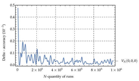
Figure 1.
Results from Table 1, for Problem 3 (in Example 1).
On the basis of Table 1 we see that the obtained results are sufficiently close to the expected results.
We conducted the check experiment. Namely, we calculated the probabilistic solution of Problem 3 at the point for , and we obtained (see Table 1). The result is improved, as expected (see Section 4). In general, increasing and N causes the improving of accuracy. For this, it is appropiate to use parallel computing systems and in this case the computational complexity of the algorithm is a matter of interest. Multicore CPUs and/or remote powerful computers can be necessary.
In Table 2 the values of the approximate solution to the Problem 2 at the same points () are given. The boundary function (21) is symmetric with respect to the plane . Respectively, in the role of , and , , the points, which are symmetric with respect to the plane , are taken. The results have sufficient accuracy for many practical problems and agrees with the real physical picture.
Table 2.
Results for Problem 2 (in Example 1).
In Table 3 the values of approximate solution to Problem 1 at the points () are given. For definition the values the formula (14) is applied, respectively, in the role of points and (), the points, which are symmetric with respect to the sphere , are taken. It is evident that the points are situated on the ray, whose beginning is at the point and located in the plane . The ray’s inclination angle with plane is equal to
Table 3.
Results for Problem 1 (in Example 1).
The points () are obtained by the inversion (6). The values are the approximate solution to Problem 2 at the points for and The obtained results agrees with the real physical picture.
Example 2.
Here in a role of infinite domain D we took again the exterior of unit sphere with the center at origin , where is a point of the surface . In considered case the boundary function has the following form
It is evident that in this case the discontinuity curves are the circles, obtained by intersection of the coordinate planes and the sphere . Actually, the sphere is divided into equal parts () by curves . In addition, in the considered case, , , are non-conductors.
Since in this case the problem domain is the same that in Example 1, therefore for the determination of intersection points () of the Wiener process trajectory and the sphere , the same algorithm, described in Example 1, is applied.
The values of the numerical solution of Problem 2 at the points () are given in Table 4. Since the boundary function (24) is symmetric with respect to the axis , therefore, in the role of (), the points which are symmetric with respect to the axis are taken. The obtained results have sufficient accuracy for many practical problems and agrees with the real physical picture.
Table 4.
Results for the Problem 2 (in Example 2).
The values of the numerical solution of Problem 1 at the points () are given in Table 5. The values are obtained by the formula (14), therefore, in the role of points and (), the points, symmetric to the sphere are taken. The points and are situated on the axis , and the points are obtained by Equation (6). The values are numerical solution to Problem 2 at the points () for and . The obtained results are agrees with the real physical picture.
Table 5.
Results for Problem 1 (in Example 2).
In this work we solved problems of type 1 when the boundary functions () are constants. This was motivated by our interest to find out how well the obtained results agree with the real physical picture. It is evident that solving Problem 1 under condition (5) is as easy as the Problem 3.
The analysis of results of numerical experiments show that the results obtained by the proposed algorithm are reliable and it is effective for the numerical solution of problems of type 1 and 3. In addition, the algorithm is sufficiently simple for numerical implementation.
6. Concluding Remarks
- 1.
- In this work, we have demonstrated that the suggested algorithm is ideally suited for numerically solving of considered problems 1 and 3. It should be noted that it is possible using this algorithm to find the solution of a problem at any point of the domain, unlike other algorithms known in the literature.
- 2.
- The algorithm does not require approximation of the boundary function, which is one of its important properties.
- 3.
- The algorithm is easy to program, its computational cost is low, it is characterized by an accuracy which is sufficient for many practical problems.
- 4.
- In the future we plan to investigate the following:
- Application of the proposed algorithm to the numerical solution of Dirichlet classical and generalized harmonic problems for the infinite space with a finite number of spherical cavities.
- Application of the MPS for the same type of problem for iregular pyramidal domains.
- Application of the MPS for the same type of problem in finite domains which are bounded by several closed surfaces.
- Application of the MPS for the same problem for infinite 2D domains with a finite number of circular holes.
Author Contributions
Conceptualization, M.Z., Z.T., N.K. and T.D.; methodology, M.Z., Z.T., N.K., T.D., J.M.S. and F.C.-A.; formal analysis, M.Z., Z.T., N.K., T.D. and F.C.-A.; investigation, M.Z., Z.T., N.K., T.D., J.M.S. and F.C.-A.; writing—original draft, M.Z., Z.T., N.K. and T.D.; writing—review and editing, J.M.S. and F.C.-A. All authors have read and agreed to the published version of the manuscript.
Funding
The Authors received no specific funding for this work.
Data Availability Statement
Not applicable.
Acknowledgments
The research was conducted in the frame of the 5-year scientific plan of the Niko Muskhelishvili Institute of Computational Mathematics.
Conflicts of Interest
The Authors declare no conflict of interests.
References
- Grinberg, G.A. Selected Questions of the Mathematical Theory of Electrical and Magnetic Phenomena; Izd. AN SSSR: Moscow, Russia, 1948. (In Russian) [Google Scholar]
- Smythe, W.B. Static and Dynamic Electricity; Hemisphere Publishing: New York, NY, USA, 1988. [Google Scholar]
- Carslaw, H.S.; Jaeger, J.C. Conduction of Heat in Solids, 2nd ed.; Oxford Science Publications; Oxford University Press: New York, NY, USA, 1988; p. 522. [Google Scholar]
- Košljakov, N.S.; Gliner, E.B.; Smirnov, M.M. The Differential Equations of Mathematical Physics; Košljakov, N.S., Ed.; Gosudarstv. Izdat. Fiz.-Mat. Lit.: Moscow, Russia, 1962; p. 767. [Google Scholar]
- Budak, B.M.; Samarskiĭ, A.A.; Tihonov, A.N. A Collection of Problems in Mathematical Physics, 3rd ed.; Nauka: Moscow, Russia, 1980; p. 687. (In Russian) [Google Scholar]
- Kantorovich, L.V.; Krylov, V.I. Approximate Methods of Higher Analysis; Benster, C.D., Translator; Interscience Publishers, Inc.: New York, NY, USA, 1958; p. xv+681. [Google Scholar]
- Koblishvili, N.; Tabagari, Z.; Zakradze, M. On reduction of the Dirighlet generalized boundary value problem to an ordinary problem for harmonic function. Proc. A. Razmadze Math. Inst. 2003, 132, 93–106. [Google Scholar]
- Zakradze, M.; Koblishvili, N.; Karageorghis, A.; Smyrlis, Y. On solving the Dirichlet generalized problem for harmonic function by the method of fundamental solutions. Semin. I. Vekua Inst. Appl. Math. Rep. 2008, 34, 24–32. [Google Scholar]
- Kublashvili, M.; Sanikidze, Z.; Zakradze, M. A method of conformal mapping for solving the generalized Dirichlet problem of Laplace’s equation. Proc. A. Razmadze Math. Inst. 2012, 160, 71–89. [Google Scholar]
- Chaduneli, A.; Zakradze, M.V.; Tabagari, Z. A method of probabilistic solution to the ordinary and generalized plane Dirichlet problem for the Laplace equation. Science and Computing. In Proceedings of the Sixth TSTC Scientific Advisory Committee Seminar (Science and Computing), Moscow, Russia, 15–19 September 2003; Volume 2, pp. 361–366. [Google Scholar]
- Chaduneli, A.; Zakradze, M.; Tabagari, Z. A computer simulation of probabilistic solution to the Dirichlet plane boundary problem for the Laplace equation in case of an infinite plane with a hole. Bull. Georgian Acad. Sci. 2005, 171, 437–440. [Google Scholar]
- Bayliss, A.; Gunzburger, M.; Turkel, E. Boundary conditions for the numerical solution of elliptic equations in exterior regions. SIAM J. Appl. Math. 1982, 42, 430–451. [Google Scholar] [CrossRef]
- Ben Belgacem, F.; Fournié, M.; Gmati, N.; Jelassi, F. On the Schwarz algorithms for the elliptic exterior boundary value problems. M2AN Math. Model. Numer. Anal. 2005, 39, 693–714. [Google Scholar] [CrossRef]
- Kanunnikova, E.A. Analytic–numerical method to solve 3D exterior boundary problems for elliptic equations. St. Petersburg Polytech. Univ. J. Phys. Math. 2014, 1, 35–38. [Google Scholar]
- Charalambopoulos, A.; Gergidis, L.N. A novel stochastic method for the solution of direct and inverse exterior elliptic problems. Quart. Appl. Math. 2018, 76, 65–111. [Google Scholar] [CrossRef]
- Stratton, J.A. Electromagnetic Theory; McGraw-Hill: New York, NY, USA, 1941. [Google Scholar]
- Lamb, H. Hydrodynamics; Cambridge University Press: Cambridge, UK, 1993. [Google Scholar]
- Kellogg, O.D. Foundations of Potential Theory; Die Grundlehren der Mathematischen Wissenschaften, Band 31; Springer: Berlin/Heidelberg, Germany, 1967; p. 384. [Google Scholar]
- Tihonov, A.N.; Samarskiĭ, A.A. Equations of Mathematical Physics; Izdat. Nauka: Moscow, Russia, 1966; p. 724. [Google Scholar]
- Zakradze, M.; Kublashvili, M.; Sanikidze, Z.; Koblishvili, N. Investigation and numerical solution of some 3D internal Dirichlet generalized harmonic problems in finite domains. Trans. A. Razmadze Math. Inst. 2017, 171, 103–110. [Google Scholar] [CrossRef]
- Dynkin, E.B.; Juškevič, A.A. Theorems and Problems in Markov Processes; Izdat. “Nauka”: Moscow, Russia, 1967; p. 231. [Google Scholar]
- Chaduneli, A.; Tabagari, Z.; Zakradze, M. On solving the internal three-dimensional Dirichlet problem for a harmonic function by the method of probabilistic solution. Bull. Georgian Natl. Acad. Sci. 2008, 2, 25–28. [Google Scholar]
- Zakradze, M.; Sanikidze, Z.; Tabagari, Z. On solving the external three-dimensional Dirichlet problem for a harmonic function by the probabilistic method. Bull. Georgian Natl. Acad. Sci. 2010, 4, 19–23. [Google Scholar]
- Zakradze, M.; Mamporia, B.; Kublashvili, M.; Koblishvili, N. The method of probabilistic solution for 3D Dirichlet ordinary and generalized harmonic problems in finite domains bounded with one surface. Trans. A. Razmadze Math. Inst. 2018, 172, 453–465. [Google Scholar] [CrossRef]
- Zakradze, M.; Kublashvili, M.; Koblishvili, N.; Chakhvadze, A. The method of probabilistic solution for determination of electric and thermal stationary fields in conic and prismatic domains. Trans. A. Razmadze Math. Inst. 2020, 174, 235–246. [Google Scholar]
- Zakradze, M.; Kublashvili, M.; Tabagari, Z.; Koblishvili, N. On numerical solving the Dirichlet generalized harmonic problem for regular n-sided pyramidal domains by the probabilistic method. Trans. A. Razmadze Math. Inst. 2022, 176, 123–132. [Google Scholar]
- Zakradze, M.; Tabagari, Z.; Sanikidze, Z.; Abramidze, E. Computer modeling of a probabilistic solution for the Dirichlet generalized harmonic problem in some finite axisymmetric bodies with a cylindrical hole. Bull. TICMI 2022, 26, 37–52. [Google Scholar]
- Vladimirov, V.S. Equations of Mathematical Physics. In Pure and Applied Mathematics; Jeffrey, A., Ed.; Littlewood, A., Translator; Marcel Dekker, Inc.: New York, NY, USA, 1971; Volume 3, p. 418. [Google Scholar]
Disclaimer/Publisher’s Note: The statements, opinions and data contained in all publications are solely those of the individual author(s) and contributor(s) and not of MDPI and/or the editor(s). MDPI and/or the editor(s) disclaim responsibility for any injury to people or property resulting from any ideas, methods, instructions or products referred to in the content. |
© 2023 by the authors. Licensee MDPI, Basel, Switzerland. This article is an open access article distributed under the terms and conditions of the Creative Commons Attribution (CC BY) license (https://creativecommons.org/licenses/by/4.0/).