Abstract
Numerical integration is a basic step in the implementation of more complex numerical algorithms suitable, for example, to solve ordinary and partial differential equations. The straightforward extension of a one-dimensional integration rule to a multidimensional grid by the tensor product of the spatial directions is deemed to be practically infeasible beyond a relatively small number of dimensions, e.g., three or four. In fact, the computational burden in terms of storage and floating point operations scales exponentially with the number of dimensions. This phenomenon is known as the curse of dimensionality and motivated the development of alternative methods such as the Monte Carlo method. The tensor product approach can be very effective for high-dimensional numerical integration if we can resort to an accurate low-rank tensor-train representation of the integrand function. In this work, we discuss this approach and present numerical evidence showing that it is very competitive with the Monte Carlo method in terms of accuracy and computational costs up to several hundredths of dimensions if the integrand function is regular enough and a sufficiently accurate low-rank approximation is available.
Keywords:
multidimensional numerical integration; highly-dimensional cubatures; Gauss-Legendre integration rule; Clenshaw-Curtis integration rule MSC:
26B15; 26B20
1. Introduction
The ability to calculate very high-dimensional integrals is crucial, for example in quantum mechanics, statistical physics, inverse problems, uncertainty quantifications, probability theory, and many other fields in science and engineering (see [1,2,3]).
To calculate such integrals accurately, we need to overcome the curse of dimensionality, which is bad scaling of the computational complexity in terms of storage and floating point operations with the number of dimensions. In the case of numerical integration, we need one function evaluation at each integration node and one floating point operation to accumulate the result, i.e., a multiplication by the quadrature weight and an addition. If a one-dimensional quadrature formula is composed of m nodes and weights, the corresponding tensor product in d dimensions is composed by nodes and weights. This exponential scaling in the number of dimensions makes this straightforward approach practically impossible except for very small values of d.
The situation is even worse if we try to decompose the integration domain into subdomains (cells) to improve the resolution or adapt the cubature rule when the integrand function shows a low regularity. Partitioning each direction into n sub-intervals leads to a tensor grid with cells and, eventually, to function evaluations and floating point operations. Even if we take only one integration node per cell by setting as in the midpoint rule, such approach to numerical integration still remains impractical. A “pedantic” example illustrates why. Setting leads to function evaluations and as many floating point operations. Assuming, very optimistically, that a function evaluation costs only one floating point operation, this approach requires about s on a teraflop machine, which virtually performs floating point operations per second. This time is about times the age of the Universe, which has been recently estimated as s (see Planck Collaboration (2020) [4]).
A non-exhaustive list of methods for multidimensional numerical integration includes the Monte Carlo method and its variants such as the quasi Monte Carlo method [5,6], and the multi-level Monte Carlo (MLMC) method [7]; the sparse grid method [8,9] and the combination technique based on sparse grids [10]; grid-based approaches such as the lattice method [11,12]. It is also worth mentioning that several software libraries are available in the public domain to address this issue, such as The Sparse Grids Matlab Kit [13], a collection of Matlab functions for high-dimensional quadrature and interpolation, based on the combination technique version of sparse grids, and PyApprox [14], which implements methods such as low-rank tensor-decomposition, Gaussian processes, and polynomial chaos expansions. A detailed presentation of these methods or a systematic review of the huge literature that is available on numerical integration are beyond the scope of this paper and we refer the interested reader to a few of the many textbooks and review papers dealing with these topics, see, e.g., [15,16,17,18] and the references therein.
A breakthrough for integrating a multivariate function on a multidimensional grid is offered by the compressive nature of low-rank tensor formats, see [19,20] for a general introduction to tensor representations and a review. The most commonly used tensor formats include the tensor train (TT) and tensor-train cross approximation [21,22], the quantized tensor train (QTT) [23], the canonical polyadic decomposition (CPD) [24], Tucker decomposition [25], and hierarchical Tucker decomposition [26]. TT-based integration has been applied in many fields, such as, just to mention a few, quantum physics and chemistry [27,28], signal processing [29], stochastics, and uncertainty quantification [30]. It is worth mentioning that recent applications of low-rank tensor formats can also be found for solving high-dimensional parabolic PDEs [31] and large ODEs with conservation laws [32]. Using such formats makes it possible to handle efficiently the function evaluation at the integration nodes and the saxpy floating point operations that accumulate the numerical value of the integral (the acronym “saxpy” stands for “scalar alpha x plus y”, i.e., multiplication by a scalar number and addition). Numerical integration of high-dimensional singular function using the tensor-train format on parallel machines is also investigated in references [33,34].
In this work, we mainly focus on the TT format, which we discuss in the next sections, and its application to composite numerical integration. Our major goal is to show that if it is possible to use an accurate low-rank tensor-train format to represent the integrand as a grid function, we can design very accurate and very efficient multivariate cubature formulas from univariate quadrature formulas in an almost straightforward way. To this end, we focus on cubatures built from the Newton-Cotes (trapezoidal and Simpson), Clenshaw-Curtis, and Gauss-Legendre formulas. However, the strategy is very general and can be adopted for all univariate integration formulas. For the sake of comparison, we consider the Monte Carlo method and its publicly available implementation provided by the library GAIL [35].
The outline of the paper is as follows. In Section 2, we discuss the problem of multidimensional numerical integration and the composite approach, where the computational domain is split into a grid of regularly equispaced cells and a univariate quadrature rule is applied inside each cell and in any direction. In Section 3, we review some basic concepts about the tensor-train format. In Section 4, we investigate the performance of our method for the integration of a set of representative functions and assess its performance. In Section 5, we offer our final remarks and discuss possible future work.
2. Multidimensional Numerical Integration
In this section, we introduce the notation of the paper and briefly review the construction of composite cubature formulas through the tensor product of univariate high-order accurate quadrature rules. First, we split the multidimensional domain into the union of hypercells, which are the tensor product of univariate partitions along the space directions. Then, inside each cell, we build the multidimensional cubature as the tensor product of univariate quadrature rules, and we characterize the accuracy of such a numerical approximation by considering the contribution of each direction to the total integration error.
2.1. Tensor Product Construction of Composite Cubature Formulas
Let be a real-valued function defined on the multidimensional hypercube . We want to design a composite integration algorithm that numerically approximates the multidimensional integral
where is the position variable along the ℓ-th direction, and is the integer index running over all the space directions. To this end, we introduce a family of multidimensional grids . We uniquely identify each member of such a family by the array of strictly positive integers . Each grid is the tensor product of d independent partitionings for , into equally spaced subintervals of , so that . We let to be the space size in the ℓ-th direction, i.e., the distance between two consecutive nodes of . We assume that tends to zero uniformly in ℓ, which implies that tends to ∞ uniformly in ℓ. We label the grid nodes of by using the multi-index , where . We let denote the set of all admissible multi-indices in accordance with the given , i.e., all possible d-uple combinations of positive integers between 1 and for the multidimensional mesh . The multidimensional grid nodes are given by
where is the position of the -th node along the ℓ-th direction, so that, for all ℓ, it holds that when and when . In view of this definition, every grid decomposes into a set of smaller hypercubes, the cells, that are isomorphic to . We denote the cell corresponding to the multi-index by , so that the “-th” cell is formally given by
Every mesh forms a finite cover of , i.e., , and the mesh cells are nonoverlapping in the sense that the d-dimensional Lebesgue measure (hypervolume) of the intersection of any possible pair of distinct cells is zero, i.e., for all , . Therefore, we can reformulate in (1) as the sum of cell subintegrals,
and devise a computer algorithm for the composite numerical integration over by assembling local multidimensional cubature rules that approximate all integrals . In the literature, the word composite (or, sometimes, compound) normally refers to the combination of one-dimensional Newton-Cotes formulas to subintegrals obtained after splitting a univariate integration domain into a finite number of nonoverlapping subdomains. Hereafter, we shall use this word to refer to a generic integration algorithm on a multidimensional tensor grid. We will consider composite formulas obtained from the Newton-Cotes as well as Gauss-Legendre and Clenshaw-Curtis quadratures. For the sake of exposition, we assume that the quadrature rule is the same in all univariate subintervals . Different integration formulas can be considered in any subinterval at the price of a more complex description of the algorithm.
Let be an m-point quadrature rule with nodes and weights for the approximation of a line integral over the reference segment . We do not require (nor exclude) that the extremal points are part of the integration nodes. We map the reference domain onto all the d one-dimensional intervals forming a given cell , identified by the multi-index . Accordingly, the -th reference node with coordinates is mapped onto the node with the ℓ-th coordinate equal to , and the corresponding weight becomes . The tensor product of the d directions provides a local subgrid of quadrature nodes inside . We denote these subgrid nodes by using the multi-index , so that
The multi-index identifies the -th cell, i.e., , and the multi-index identifies the quadrature node inside . In fact, the index labels the -th node of the m-node univariate quadrature rule along the ℓ-th space direction, denoted by the superscript in . We denote the set of all possible values of by . The nodes are all located in the interior of if the corresponding reference nodes are inside as in the case of the Gauss-Legendre integration rules. Figure 1 illustrates the notation for the case with .
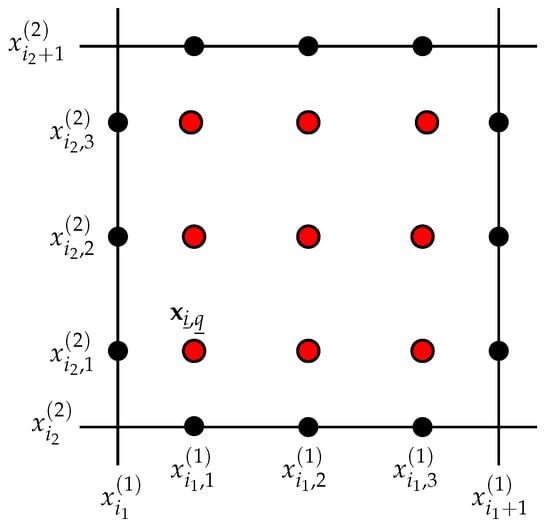
Figure 1.
Notation. For , we show the generic cell , with ; the univariate quadrature nodes (black dots) with coordinate , with , , which corresponds to the 3-point Gauss–Legendre integration rule; the cubature nodes inside the cell (red dots) are provided by the tensor product of the one-dimensional quadrature nodes along the directions . To make the figure easily readable, we show all the quadrature and cubature nodes relative to cell , but we report only the coordinates of the quadrature nodes at the bottom and left sides, and the coordinates of the internal bottom-left node, i.e., , with , and .
The integration weight associated with the -th node of the -th cell is the product of the one-dimensional weights identified inside by , where for . We have that
where is the weight associated to the -th node along the (univariate) ℓ-th direction of cell . In Equation (3), we do not need to label the weights with the cell index since we assumed that the integration formula is the same in every cell, and so are the weights.
Finally, our composite cubature rule on the multidimensional mesh is obtained by applying the local cubature rule to all cells of grid and adding the results, so that
where we take the summation over all the possible instances of the multi-indices and .
2.2. Accuracy of Multidimensional Cubature Formulas on the Reference Cell
The numerical integration error that characterizes the composite numerical integration formula with partitionings of reads as:
An estimate of such error is fundamental to assess the accuracy of our cubature formulas. We can estimate the accuracy of a multidimensional numerical integration rule if we know the accuracy of the univariate quadrature rule used in each space direction of the tensor product construction. Let be the multidimensional reference cell, and with for , the multidimensional position vector in . For all integers , we consider the notation and , with the convention that and . Using this notation, we introduce the partition . Similarly, we introduce the notation and . Again, for consistency, we say that , , and we split the d-dimensional multi-index as . Next, we consider the reduced domain of integration , which contains all the vectors such that , and the reduced set of integration indices that contains all -sized multi-indices of the form . Finally, we set , and introduce the partial numerical integration formula for the function :
where we apply the quadrature formula in all directions from ℓ to d. Finally, we define the partial cubature rule that integrates exactly on the first directions and numerically along the remaining ones from ℓ to d, so that for we write that
We complete this definition by setting and . To ease the notation, hereafter we will write instead of . The integration error on is the telescopic sum
Since it holds that , and , we split the integral over as follows
Using this splitting, we find that
The univariate quadrature rule is applied in the ℓ-th direction to the integral inside the brackets in the last step. Let be an upper bound on the integration error along direction ℓ, clearly dependent on the regularity of , so that
for all points and all sets of quadrature nodes along the remaining directions . Since the quadrature weights are positive (see Remark 1 below), we find that
since for we have the summations and it holds that
being the -dimensional measure of and the one-dimensional measure of the reference interval . An upper bound on the error of the multidimensional reference domain is thus given by
In view of (6), we only need to know for , i.e., the accuracy of the univariate quadrature in every direction to estimate the error of the multidimensional cubature formula. Let . Then, we find that
where the constant C depends on d but is independent of m.
Remark 1
(Weight positivity). The weights of the Clenshaw-Curtis quadratures can be computed using the formulas given in [36] Equations (4) and (5), and it is immediate to deduce that they are all positive. A straightforward argument allows us to prove that the weights of the Gauss-Legendre quadratures must also be strictly positive. Consider the polynomial
Its integral over must be strictly positive, independently of the number of points m, since for all . The m-point Gauss-Legendre quadrature rule integrates exactly since is a polynomial of degree . Noting that for all by construction, we find that
This relation implies that since , and the positivity of all integration weights follows by repeating this argument for all i from 1 to m. The weights for the Clenshaw-Curtis () and Gauss-Legendre () formulas used for the numerical experiments of Section 4 are reported in Appendix A.
Finally, we note the weights of two Newton-Cotes formulas used in this work, i.e., the trapezoidal and Simpson quadrature rule, are positive. However, the weight positivity is not a property of this family of quadrature rules, so we can apply the argument discussed in this section to the trapezoidal and Simpson quadrature rule but not to all the Newton-Cotes formulas.
For the cubature families built upon the Newton-Cotes (trapezoidal and Simpson) formulas, Clenshaw-Curtis formulas, and Gauss-Legendre formulas, the upper bound depends on the number of quadrature nodes m and the regularity of . We summarize these results, which are easily available from the literature (see [16,17,18,37]), in the following theorems. We assume that the univariate integrand function and its first derivatives , up to some given integer , have (at least) the regularity that is mentioned in each theorem’s assertion.
Theorem 1
(Newton-Cotes formulas for ).
- Let ; then, the Newton-Cotes formula with two integration nodes (, trapezoidal rule) satisfiesfor some point .
- Let ; then, the Newton-Cotes formula with three integration nodes (, Simpson rule) satisfiesfor some point .
Proof.
The theorem statements follow from [37] (Equations (9.12) and (9.16)), by setting for the size of the reference one-dimensional integration cell . □
Theorem 2
(Clenshaw-Curtis formulas). Let the univariate integrand function and its derivatives be absolutely continuous on the integration domain . Let the ν-th derivative have bounded variation for some integer number . Then, the m-point Clenshaw-Curtis quadrature applied to on the integration domain satisfies
where C is a constant independent of m.
Proof.
The theorem statement is adapted from [38] (Theorem 5.1) and the first statement of [18] (Theorem 19.4) by setting the number of quadrature nodes to m. □
Theorem 3
(Gauss-Legendre formulas). Let the univariate integrand function and its derivatives be absolutely continuous on the integration domain . Let the ν-th derivative have bounded variation for some integer number . Then, the m-point Gauss-Legendre quadrature applied to on the integration interval satisfies
where C is a constant independent of m.
Proof.
The theorem statement is adapted from [38] Theorem 5.1 and the second statement of [18] Theorem 19.4 by setting the number of quadrature nodes to m. □
2.3. Accuracy of Composite Cubature Formulas for Multidimensional Numerical Integration
Applying a scaling argument to a local estimate of the approximation error and summing over all the mesh cells, we obtain the upper bound on the integration error of the Newton-Cotes schemes. The error estimates depend on the regularity of . We assume that f in each formula has (at least) the regularity shown by its right-hand side infinity norm . We denote again the partial derivatives of order of the scalar function f by .
Theorem 4 (Convergence of composite quadrature formulas).
Let , and . Under the same assumptions of Theorem 1, it holds that
- Composite Newton-Cotes formulafor , (trapezoidal rule);
- Composite Newton-Cotes formulafor , (Simpson rule).
Moreover, under the assumption that , it holds that
- Composite Clenshaw-Curtis formulasfor ;
and under the assumption that , it holds that
- Composite Gauss-Legendre formulasfor .
The positive constant factor C is independent of (so, on the mesh size parameter h), but can depend on the number of dimensions d.
Proof.
The theorem statements follow from an interpolation error estimate and a scaling argument. We split the one-dimensional domain of integration into N equispaced subintervals of size , so that and . Accordingly, we decompose the integral of and its numerical approximation via the m-node quadrature rule as the sum of local contributions over the N subintervals:
Then, we remap every subinterval onto the reference interval . Thus, for all and such that it holds that (the subindex “k” in the symbol “” indicates that this is the image of the restriction of f to through the coordinate mapping ). For any positive integer , a straightforward calculation shows that
We rewrite the exact and approximate integration formulas on the reference interval as follows:
where the summation is taken on all the quadrature nodes (and using obvious definitions of the functionals “” and “”). We bound the error on the k-th cell as follows
To estimate , we introduce the polynomial interpolation of the integrand function at the m quadrature nodes on the reference interval . This interpolation is the unique polynomial of degree in that takes the same values of at the m quadrature nodes , i.e., for . If we apply to and , we obtain the same integral approximation because the quadrature rule depends only on the quadrature node values . Moreover, the quadrature rule is of interpolatory type and is exact on all polynomials of degree (up to) . Therefore, we find that
Using the formula above, we immediately find that
where is the interpolation error over the reference cell . The regularity assumptions of the theorem imply that is times continuously differentiable for some integer , whose value changes according to the quadrature formula. From standard arguments of polynomial interpolation theory, we know that , where denotes the ∞-norm of , the -th derivative of on , and C is a real, positive constant that may depend on the number of quadrature nodes m. Using the derivative scaling (14), we find that
where denotes the ∞-norm of on . Here, C is a constant independent of h, but that may still depend on the number of quadrature nodes m. Summing over all the cells and noting that , we find the following estimate for the integration error in each direction:
The theorem’s assertions follow on first setting for the trapezoidal rule and for the Simpson rule (in accordance with Theorem 1), and setting for the Clenshaw-Curtis formulas and for the Gauss-Legendre formula (in accordance with the theorem’s regularity assumptions), and then taking the maximum over all the directions. □
Remark 2.
The estimate for the Gauss-Legendre formulas can also be derived in a straightforward way by using the formula for “” in [39] (Example 5.2, page 146) and setting directly “” (according to the notation used therein). Note, however, that the derivation of such a formula is not presented in [39].
3. Low-Rank TT Cross Approximation and Numerical Integration of a Multidimensional Function
In this section, we briefly review the low-rank tensor-train approximation of a multidimensional grid function and its application to the numerical integration. An extensive presentation and discussion of these concepts and algorithms can be found in [21,22].
3.1. Tensor-Train Decomposition: Basic Definitions and Properties
A d-order tensor is a multidimensional array whose entries are addressed by d indices as
according to a notation used in MATLAB@ [40] and the Python programming language [41]. Hereafter, we shall refer to the integers as the mode sizes. The set of all d-dimensional arrays with the arithmetic operations of addition and multiplication by a scalar number, which we assume to be defined in the natural way, is a linear space. We endow such a linear space with the inner (dot) product and induced norm
for all , and where the summation runs over the set of all admissible values of the multi-index . The norm is usually called the Frobenius norm of A.
We say that the d-order tensor A admits a tensor-train representation if there exists a -tuple of strictly positive integers , with , and d three-dimensional tensors , , such that
for all , . The tensors are called the TT cores and the integers the TT ranks (also known as the compression ranks) of the tensor-train representation. Since the tensors and are two-dimensional arrays, i.e., matrices, and the right-hand side of (16) is a scalar number. Moreover, each factor for any fixed is a matrix with size , so that we can reformulate (16) in the compact matrix multiplication form given by
which allows for a faster implementation using BLAS level-3 routines [42].
The storage of the tensor-train representation of A requires real numbers. If n and r are convenient upper bounds of all the mode sizes and TT ranks, so that and for all ℓ, the storage is proportional to instead of of the full format representation.
The tensor-train representation of a tensor A is related to an exact or approximate skeleton decomposition of its unfolding matrices , , cf. [21]. The ℓ-th unfolding matrix is defined by suitably remapping the entries of A into a matrix with size . To this end, we consider the integer-valued functions , , which are iteratively defined as
Then, we set
The existence of an exact TT decomposition of a tensor with compression ranks equal to the ranks of its matrix unfoldings is proved in [21]. Such compression ranks are the smallest possible ones among all possible exact tensor-train decompositions of A. The problem of computing approximate tensor-train decompositions with smaller ranks is addressed in [22]. In particular, if all the unfolding matrices of tensor A can be approximated by rank- matrices through an approximate skeleton decomposition with accuracy so that
then, there exists an approximate tensor with compression ranks satisfying
In the numerical experiments of Section 4, we shall consider the low-rank tensor-train approximation of the grid functions given by using the TT cross interpolation of multidimensional arrays proposed in [22]. The TT cross-skeletal decomposition allows us to approximate a multivariate function using only a few entries of the tensor array resulted from the function sampling at the grid nodes, thus avoiding working with the array containing the full multidimensional grid function.
3.2. Numerical Integration of a Low-Rank Tensor-Train Representation of a Multidimensional Grid Function
For any mesh cell , we collect the nodes and weights defining the elemental multidimensional integration rule in the pair , where is the set of the quadrature nodes and is the set of quadrature weights. The global integration rule in (4) is associated with , so that, for any cell index , it holds that and , where we denote the restriction of quantity to cell as . We represent the grid function given by sampling function f at the nodes of a generic d-dimensional grid X by the d-dimensional tensor . If , every index runs from 1 to . The nodes of are not equispaced if the local multidimensional cubature rule is built by taking the tensor product of univariate quadrature rules with non-equispaced nodes such as the Clenshaw-Curtis and Gauss-Legendre formulas. The integration formula (4) can be rewritten as the tensor inner product
Tensor has compression ranks equal to 1, and if we know a TT decomposition of with compression ranks , we compute the composite cubature rule on mesh using Algorithm 1 with a computational cost proportional to . Recalling again the uniform upper bounds and , we find that the storage scales up like . The computational complexity is thus polynomial in the mode sizes and compression ranks, and under the (strong) assumption that the error in (18) and (19) is small for all ℓ, the computational complexity may depend only linearly on the number of dimensions. We prove this result in the following theorem.
| Algorithm 1: Tensor-Train Cubature Algorithm. |
 |
Theorem 5.
Let admit the low-rank approximation in the tensor-train format so that
where , for , are the tensor-train ranks and , for , is the index running through all the quadrature nodes of the intervals along the direction ℓ. Then, to compute the numerical cubature (20) using Algorithm 1 we need saxpy operations.
Proof.
Let be the one-dimensional -sized vector collecting all the weights of all quadrature nodes along the direction ℓ. Then, we write the cubature rule (20) as
where is the mode-2 product between vector and the tensor-train core tensor , i.e, the contraction along the ℓ-th mode index. For every pair of indices of the contracted core , the contraction requires saxpy operations, and since is an -sized matrix, the contraction of all the d cores requires of such operations. Eventually, the calculation proceeds as a sequence of vector-matrix product from left to right between a temporary intermediate one-dimensional -sized array and the two-dimensional -sized matrix for , thus requiring other saxpy operations. □
Remark 3.
If tensor admits a low-rank approximation with compression ranks , we have the even better scaling proportional to .
Remark 4.
Using the TT cross interpolation algorithm for multidimensional arrays [22] makes it possible to compute such an approximate TT decomposition of using only a very small fraction of the grid values of and without pre-computing and storing the full tensor . For the details of this algorithm and its practical implementation, we refer again to [22].
We characterize the accuracy of this approximation by introducing the tolerance factor , which is such that . The tolerance factor has clearly an influence on the ranks of the tensor-train approximation of the multidimensional tensor of the grid function values, e.g., , and we can expect that a smaller tolerance implies bigger ranks. The interplay between tolerance and the ranks is crucial to obtain an efficient integration algorithm. If instead of computing , we compute , where is an approximation of f represented by , and we use the linearity of , we immediately find the bound on the integration error given by
Assuming for simplicity that for , so that we have the same number of points n corresponding to partitions in every direction, we note that
Using this fact, definition (20) and the Cauchy-Schwarz inequality, we find that
If , we can neglect the last term of (21), and we find that , i.e., the convergence properties of the cubature remain essentially the same even if integrate instead of f.
4. Numerical Experiments
The Newton-Cotes (trapezoidal and Simpson rules), Clenshaw-Curtis, and Gauss formulas are all of the interpolatory type. In fact, they can be derived by integrating the polynomial interpolant supported by the quadrature nodes and are characterized by the polynomial degree and the following exactness property [15]. For any integer ,
- the Newton-Cotes formulas with points (trapezoidal rule) and points (Simpson’s rule) integrate exactly the polynomials of degree 1 and 3, respectively;
- the m-point Clenshaw-Curtis formula integrates exactly all polynomials of degree up to ;
- the m-point Gauss-Legendre formula integrates exactly all polynomials of degree up to .
These exactness properties readily extend to the multidimensional compound cubature. In this section, we assess the performance of our strategy to build such cubatures by investigating the “h” and the “p” convergence of the method (using a terminology widely adopted in the finite element method). Here, is the (uniform) step size of each univariate partition of the tensor product grid, and is the number of intervals of every partition. Moreover, we set the tolerance factor , and we note that the observed rank is typically between 5 and 10.
4.1. Test Case 1: h-Convergence of a Smooth Function
The three panels in Figure 2 show the log-log plot of the error curves versus the number of intervals per direction N for the numerical integration of the multidimensional function
- Test Case 1:
on the integration domain .
We consider . We perform the numerical integration using (i) the Newton-Cotes formulas (trapezoidal and Simpson quadrature rules); (ii) the Clenshaw-Curtis formula with ; (iii) the Gauss-Legendre formula with . The convergence rate is expected to be proportional to (trapezoidal rule); (Simpson rule); (Clenshaw-Curtis rule); (Gauss-Legendre rule), and is shown by the slope of the triangle close to each curve. The slopes of the error curves reflect the numerical orders of convergence, and Figure 2 shows that these slopes are in agreement with the theoretical expectations. We also note that the convergence behavior seems to be unaffected by the number of dimensions.

Figure 2.
Test Case 1. Relative approximation error curves versus the number of intervals per direction N for the numerical integration of a d-dimensional polynomial of degree 10, , using (i) Newton–Cotes formulas (trapezoidal and Simpson quadrature rules); (ii) Clenshaw–Curtis formula with ; (iii) Gauss–Legendre formulas with . The expected convergence rate is shown by the number close to the triangular shapes and is proportional to (trapezoidal rule); (Simpson rule); (Clenshaw-Curtis rule); (Gauss-Legendre rule).
4.2. Test Cases 2 and 3: h-Convergence and Integration of Multidimensional Exponential Functions
In the second and third test cases, we consider the Gauss bell-shaped function and the exponential function, which we denote as Genz-4 and Genz-5 following the nomenclature introduced in [43,44]:
- Test Case 2: Genz-4:
- Test Case 3: Genz-5:
In Figure 3 and Figure 4, we show the log-log plots of the error curves versus the number of intervals N per direction for the numerical integration of the d-dimensional version of these functions. We consider . We perform the numerical integration using the (i) trapezoidal formula (); (ii) Simpson formula (); (iii) Clenshaw-Curtis formula (); (iv) Gauss-Legendre formula (. The expected convergence rate, still reflected by the slope of the triangles near each curve, is expected to be proportional to (trapezoidal rule) and (Simpson, Clenshaw-Curtis, and Gauss-Legendre rules). As in the previous test case, the numerical slopes are in agreement with the theoretical slopes, still shown by the triangle in each plot. The number of dimensions plays, however, a more significant role than the previous test case, and the constant factor that appears in every error bound, see Theorem 4, changes with d. This behavior is the same for all the cubature schemes that we consider in this test case.
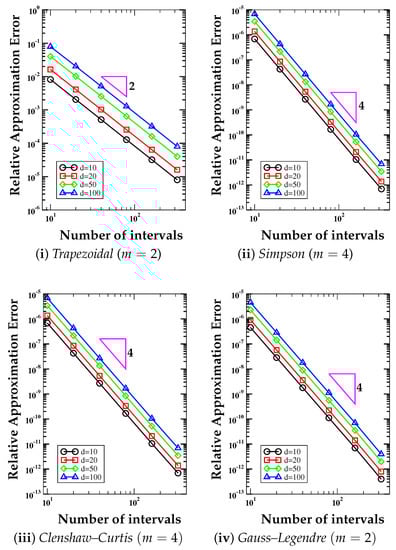
Figure 3.
Test Case 2. Relative approximation error curves versus the number of intervals N per direction for the numerical integration of a d-dimensional Gaussian bell-shaped function (Genz-4), , using the (i) trapezoidal formula (); (ii) Simpson formula (); (iii) Clenshaw–Curtis formula (); (iv) Gauss–Legendre formulas (. The expected convergence rate is shown by the number close to the triangular shapes and is proportional to (trapezoidal rule) and (Simpson, Clenshaw-Curtis, and Gauss-Legendre rules).
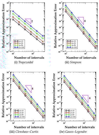
Figure 4.
Test Case 3. Relative approximation error curves versus the number of intervals N per direction for the numerical integration of a d-dimensional exponential function (Genz-5), , using the (i) trapezoidal formula (); (ii) Simpson formula (); (iii) Clenshaw–Curtis formula (); (iv) Gauss–Legendre formulas (. The expected convergence rate is shown by the number close to the triangular shapes and is proportional to (trapezoidal rule) and (Simpson, Clenshaw–Curtis, and Gauss–Legendre rules).
4.3. Test Case 4: p-Convergence and Integration of Multidimensional Exponential Functions
In Figure 5, we show the linear-log plots of the error curves that are obtained by applying the cubature rules built using the univariate Clenshaw-Curtis formula (right column) and the Gauss-Legendre formula (left column). The two panels on top refer to the numerical integration of the Genz-4 function, while the two panels at the bottom refer to the numerical integration of the Genz-5 function. We carry out all calculations on a very coarse grid with only two intervals per direction, so the resolution is (d times), and we have a total of multidimensional cells. The numerical integration is performed for . We build the cubature rules using the univariate Clenshaw-Curtis and Gauss-Legendre formulas with m integration nodes with . The four plots of Figure 5 show that the convergence of the Clenshaw-Curtis and Gauss-Legendre formula is (roughly) proportional to for some positive number .
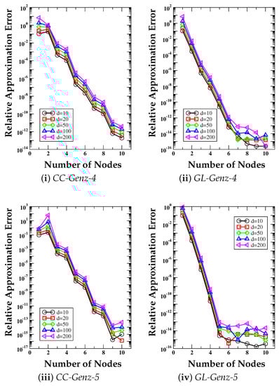
Figure 5.
Test Case 4. Relative approximation error curves versus the number of integration nodes m of the univariate quadrature rule for the numerical integration of a d-dimensional Gaussian bell-shaped function (Genz-4, top panels) and the exponential function (Genz-5, bottom panels). We integrate both multidimensional functions on a grid with . In panels (i) and (iii), we use the m-points Clenshaw–Curtis (CC) formulas; in panels (ii) and (iv), we use the m-points Gauss–Legendre (GL) formulas. In all cases, we consider .
4.4. Test Case 5: Adaptivity for Numerical Integration of Multidimensional, Weakly Singular Functions
In this test case, we show how we can adapt our cubature formulas to the integration of functions with lower regularity. For this test case, we present only the results obtained with Gauss-Legendre quadrature rule. The results obtained with the Clenshaw-Curtis quadrature rule are essentially the same. To this end, we consider the so-called ANOVA function, see, for example, [6]:
- Test Case 5: ANOVA:
This function is only continuous on the integration domain , as all its directional derivatives have a singularity at the point with ℓ-th coordinate equal to . We assume that for all directional index . We perform the numerical integration versus the number of dimensions, using the Gauss-Legendre formula with 2 nodes, and the equispaced grids with partitions per direction. When , the left panel of Figure 6 shows that the numerical integration with the partition does not provide a good result. The reason for this behavior is that the singularity of the integrand is inside the (unique) integration cell. However, when we consider the tensor product grid with and 4 partitions per direction, the cubature rule provides a very accurate result with an error of the order of the machine’s precision. In such a case, the multidimensional grid decomposes the computational domain in such a way that the integrand singularity matches with the cell interfaces. Therefore, we are integrating over subdomains where the integrand is actually smooth, and since the Gauss-Legendre is exact on linear polynomials the final error must be zero up to the machine’s precision. This same behavior is reflected by the right panel of Figure 6, which refers to the integration of the ANOVA function with . In such a case, only the partition with cells per direction matches the location of the singularity at a cell interface. This is the only situation in this test case that can be expected to provide a numerical value for the integral that is close to the machine precision, as reflected by the numerical results.
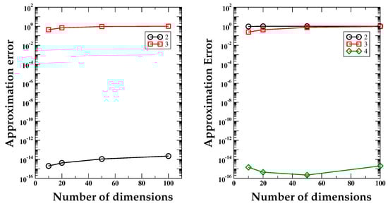
Figure 6.
Test Case 5. Approximation error curves versus the number of dimensions d for the numerical integration of a singular function using different partitions of the multidimensional domains. We apply the Gauss–Legendre formula with . The plot on the left shows the errors computed using grids with two and three partitions per direction, and the singularity located at the middle of every direction. The plot on the right shows the same test case with grids with two, three, and four partitions per direction, and the singularity located at the three-quarter mark of every direction. When the singularity is located at an interface between two cells, the integration formula is exact and the error is of the order of the machine’s precision, independent of the number of dimensions.
4.5. Test Case 6: Integration of a High-Degree Polynomial and a Function with a Singular High-Order Derivative
We consider the function
- Test Case 6:
defined on the integration domain Ω = [0, 1]d, where is the univariate Chebyshev polynomial of the first kind of degree μ along the direction l. The exact value of the integral of the function is reported in Table 1. We write the first nine derivatives along the direction of this function as follows:
where and is the k-th derivative of . Function f(x) and its first μ − 1 derivatives , 1 ≤ k ≤ μ − 1, are clearly continuous at the singular point and since the other directions are not affected by the singularity, which is only along the hyperplane all these functions are continuous on Ω. Instead, the μ-th derivative along is singular at , as it reads

Table 1.
Test Case 6: exact value of the integral of the function for μ = 1,…,10.
The regularity of f is sufficient to ensure the convergence of the Gauss-Legendre integration formula for m = 1,…, μ since according to Theorem 4, we only need a regularity up to fm. When m ≥ μ/2, the Gauss-Legendre quadrature integrates exactly all polynomials of degree up to μ − 1, and we expect to see the integration error at the machine precision level. Figure 7 shows the linear-log plot of the error curves versus the number of nodes m. For comparison, we consider a tensor product mesh with two partitions per direction, so that the singularity coincides with a cell interface that is orthogonal to the first spatial direction. In this last situation, the singularity does not affect the accuracy of the numerical integration, as discussed in Test Case 5. The expected behavior is confirmed for d = 10.
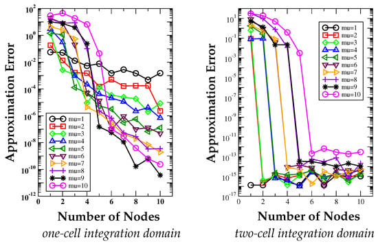
Figure 7.
Test Case 6. Approximation error curves versus the number of nodes m for the numerical integration of the combination of a singular function and the Chebyshev degree-10 polynomial of the first kind on a d = 10 dimensional domain.
4.6. Test Case 7: Efficiency Benchmarks through a Comparison with Monte Carlo Methods
Figure 8 shows the log-log plot of the error curves versus the elapsed time. We compare the performance of the strategy proposed in this paper using the Gauss-Legendre quadrature formula and the performance of two Monte Carlo integration methods (MC Lattice, MC Sobol, see [35]). These two variants of the Monte Carlo method are provided by the library GAIL [35]. The elapsed time is measured in seconds and the number of dimensions of the integrated function, d, is indicated below each panel. The numerical integration is performed on function Genz-2 (see [43,44]):
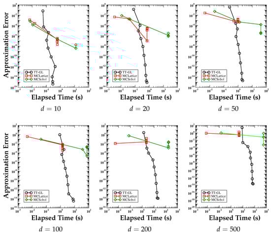
Figure 8.
Test Case 7. Approximation error curves versus the elapsed time. We compare the performance of the strategy proposed in this paper and that of two Monte Carlo integration methods (MC Lattice, MC Sobol). The elapsed time is measured in seconds and the number of dimensions of the integrated function, d, is indicated below each panel. Each panel shows that our integration strategy is more efficient than the Monte Carlo method.
- Test Case 7: Genz-2:
on a d-dimensional grid with d = 10, 20, 50, 100, 200, 500. These results show that the numerical integration error of the proposed cubature formula can be up to 10 orders of magnitude smaller for comparable elapsed times.
5. Conclusions
In this paper, we discuss an approach to extend the one-dimensional integration rule to a multidimensional grid and presented numerical evidence demonstrating its effectiveness. The straightforward extension of a one-dimensional quadrature to multidimensional grids by the tensor product of the spatial directions is deemed practically impossible for dimensions greater than three or four. The computational burden in terms of storage and floating point operations grows exponentially with the number of dimensions due to the curse of dimensionality. By employing a low-rank tensor-train representation of the integrand functions, however, the tensor product method can be utilized effectively for high-dimensional numerical integration. We assessed the effectiveness of this approach by applying it to the numerical integration of a selected set of multidimensional functions. In particular, the composite integration technique can be competitive with the Monte Carlo method in terms of accuracy and computational costs if the integrand function is sufficiently regular and admits a low-rank tensor train. We obtain such a low-rank representation by applying the TT cross interpolation algorithm, which provides an approximation of the multidimensional tensor collecting the values of the integrand function at the integration nodes. We proved that the accuracy of our composite numerical cubatures is dominated by the “standard” numerical integration error, which depends on the regularity of the integrand function whenever such an error is much bigger than the error introduced by the TT cross approximation algorithm. An open issue is the characterization of the functional interpolation that the TT cross approximate tensor provides. We can assume that this functional interpolation belongs to a subspace of a finite-dimensional approximation space that we can construct, for example, by the tensor product of univariate polynomials, piecewise polynomials interpolations, or similar constructions. If we had a characterization of this subspace, then we could analyze the numerical integration error directly through the function approximation based on the TT cross interpolation algorithm. We will investigate this topic in our future work.
Author Contributions
Conceptualization, B.A., G.M., E.W.S., P.M.D.T. and R.G.V.; Methodology, B.A., G.M., E.W.S., P.M.D.T. and R.G.V.; Validation, B.A., G.M., E.W.S., P.M.D.T. and R.G.V.; Writing—original draft, B.A., G.M., E.W.S., P.M.D.T. and R.G.V.; Writing—review & editing, B.A., G.M., E.W.S., P.M.D.T. and R.G.V. All authors have read and agreed to the published version of the manuscript.
Funding
This research was funded by Laboratory Directory Research and Development (LDRD) grant number 20230067DR and 20210485ER.
Institutional Review Board Statement
This document has been approved for public release as the Los Alamos Technical Report LA-UR-22-29661.
Data Availability Statement
Not applicable.
Acknowledgments
This work was partially supported by the Laboratory Directed Research and Development (LDRD) program of Los Alamos National Laboratory under Grants 20190020DR, 20230067DR and 20210485ER, and in part by LANL Institutional Computing Program. Los Alamos National Laboratory is operated by Triad National Security, LLC, for the National Nuclear Security Administration of U.S. Department of Energy (Contract No. 89233218CNA000001). This article has been authored by an employee of the National Technology & Engineering Solutions of Sandia, LLC under Contract No. DE-NA0003525 with the U.S. Department of Energy (DOE). The employee owns all right, title and interest in and to the article and is solely responsible for its contents. The United States Government retains, and the publisher, by accepting the article for publication, acknowledges that the United States Government retains a non-exclusive, paid-up, irrevocable, worldwide license to publish or reproduce the published form of this article or allows others to do so, for United States Government purposes. The DOE will provide public access to these results of federally sponsored research in accordance with the DOE Public Access Plan https://www.energy.gov/downloads/doepublic-access-plan.
Conflicts of Interest
The authors declare no conflict of interest.
Appendix A. Clenshaw-Curtis and Gauss-Legendre Quadrature Rules
Clenshaw-Curtis quadratures can be derived through an expansion of the integrand function on Chebyshev polynomials, or, equivalently, through the change of variables x = cos θ and, then, applying a discrete cosine transform (DCT) approximation for the cosine series. For the readers’ convenience, we report the value of the Clenshaw-Curtis quadrature nodes and weights of order 2, 3, 4, which we used in our numerical experiments, in Table A1.
Table A1.
Nodes and weights of the Clenshaw-Curtis quadrature formulas of order 2, 3, and 4 on the interval [−1, 1].
Table A1.
Nodes and weights of the Clenshaw-Curtis quadrature formulas of order 2, 3, and 4 on the interval [−1, 1].
| Clenshaw-Curtiss-2 | Clenshaw-Curtiss-3 | Clenshaw-Curtiss-4 | ||||
|---|---|---|---|---|---|---|
| Nodes | Weights | Nodes | Weights | Nodes | Weights | |
| 1 | −1 | 1 | −1 | 1/3 | −1 | 1/9 |
| 2 | 1 | 1 | 0 | 4/3 | −1/2 | 8/9 |
| 3 | 1 | 1/3 | 1/2 | 8/9 | ||
| 4 | 1 | 1/9 | ||||
The nodes , i = 1,…, n, of the Gauss-Legendre quadrature of order n are the n roots of , the univariate Legendre polynomial of degree n defined on the reference interval [−1, 1]. The corresponding weight is given by the formula . For the readers’ convenience, we report the Gauss-Legendre quadrature formulas of order 1, 2, and 3, which we used in our numerical experiments, in Table A2.
Table A2.
Nodes and weights of the Gauss-Legendre quadrature formulas of order 1, 2, and 3 on the interval [−1, 1].
Table A2.
Nodes and weights of the Gauss-Legendre quadrature formulas of order 1, 2, and 3 on the interval [−1, 1].
| Clenshaw-Curtiss-1 | Clenshaw-Curtiss-2 | Clenshaw-Curtiss-3 | ||||
|---|---|---|---|---|---|---|
| Nodes | Weights | Nodes | Weights | Nodes | Weights | |
| 1 | 0 | 2 | −1/ | 1 | − | 5/9 |
| 2 | 1/ | 1 | 0 | 8/9 | ||
| 3 | 5/9 | |||||
References
- Brooks, S.; Gelman, A.; Jones, G.L.; Meng, X.L. Handbook of Markov Chain Monte Carlo; Handbooks of Modern Statistical Methods; Chapman & Hall/CRC: Boca Raton, FL, USA, 2011. [Google Scholar]
- Stuart, A.M. Inverse problems: A Bayesian perspective. Acta Numer. 2010, 19, 451–559. [Google Scholar] [CrossRef]
- Meyer, H.D.; Manthe, U.; Cederbaum, L.S. The multi-configurational time-dependent Hartree approach. Chem. Phys. Lett. 1990, 165, 73–78. [Google Scholar] [CrossRef]
- Aghanim, N.; Akrami, Y.; Ashdown, M.; Aumont, J.; Baccigalupi, C.; Ballardini, M.; Banday, A.J.; Barreiro, R.B.; Bartolo, N.; Basak, S.; et al. Planck 2018 results. Astron. Astrophys. 2020, 641, A6. [Google Scholar] [CrossRef]
- Barbu, A.; Zhu, S.C. Monte Carlo Methods; Springer: Berlin/Heidelberg, Germany, 2020; pp. 1–17. [Google Scholar]
- Wang, X.; Fang, K.T. The effective dimension and quasi-Monte Carlo integration. J. Complex. 2003, 19, 101–124. [Google Scholar] [CrossRef]
- Giles, M.B. Multilevel Monte Carlo methods. Acta Numer. 2015, 24, 259–328. [Google Scholar] [CrossRef]
- Gerstner, T.; Griebel, M. Numerical integration using sparse grids. Numer. Algorithms 1998, 18, 209. [Google Scholar] [CrossRef]
- Novak, E.; Ritter, K. High dimensional integration of smooth functions over cubes. Numer. Math. 1996, 75, 79–97. [Google Scholar] [CrossRef]
- Griebel, M.; Schneider, M.; Zenger, C. A combination technique for the solution of sparse grid problems. In Iterative Methods in Linear Algebra; de Groen, P., Beauwens, R., Eds.; IMACS, Elsevier: Amsterdam, The Netherlands, 1992; pp. 263–281. [Google Scholar]
- Sloan, I.H. Lattice methods for multiple integration. J. Comput. Appl. Math. 1985, 12–13, 131–143. [Google Scholar] [CrossRef]
- Sloan, I.H.; Joe, S. Lattice Methods for Multiple Integration; Oxford University Press: Oxford, UK, 1994. [Google Scholar]
- Piazzola, C.; Tamellini, L. The Sparse Grids Matlab kit—A Matlab implementation of sparse grids for high-dimensional function approximation and uncertainty quantification. arXiv 2022, arXiv:2203.09314. [Google Scholar]
- Jakeman, J.D. PyApprox Software Library. Available online: https://sandialabs.github.io/pyapprox/index.html (accessed on 1 December 2022).
- Cools, R. Constructing cubature formulae: The science behind the art. Acta Numer. 1997, 6, 1–54. [Google Scholar] [CrossRef]
- Davis, P.J.; Rabinowitz, P.; Rheinbolt, W. Methods of Numerical Integration, 2nd ed.; Computer Science and Applied Mathematics; Elsevier Inc.: Amsterdam, The Netherlands; Academic Press: Cambridge, MA, USA, 1984. [Google Scholar]
- Brass, H.; Petras, K. Quadrature Theory; Mathematical Surveys and Monographs 178; American Mathematical Society: Providence, RI, USA, 2011. [Google Scholar]
- Trefethen, L.N. Approximation Theory and Approximation Practice; Society for Industrial and Applied Mathematics: Philadelphia, PA, USA, 2013. [Google Scholar] [CrossRef]
- Hackbusch, W. Tensor Spaces and Numerical Tensor Calculus, 1st ed.; Springer Series in Computational Mathematics 42; Springer: Berlin/Heidelberg, Germany, 2012. [Google Scholar]
- Hackbusch, W. Numerical tensor calculus. Acta Numer. 2014, 23, 651–742. [Google Scholar] [CrossRef]
- Oseledets, I.V. Tensor-Train decomposition. SIAM J. Sci. Comput. 2011, 33. [Google Scholar] [CrossRef]
- Oseledets, I.; Tyrtyshnikov, E. TT-cross approximation for multidimensional arrays. Linear Algebra Its Appl. 2010, 432, 70–88. [Google Scholar] [CrossRef]
- Khoromskij, B.N. O(dlog n)-quantics approximation of N-d tensors in high-dimensional numerical modeling. Constr. Approx. 2011, 34, 257–280. [Google Scholar] [CrossRef]
- Savostyanov, D.V. Fast revealing of mode ranks of tensor in canonical form. Numer. Math. Theory Methods Appl. 2009, 2, 439–444. [Google Scholar] [CrossRef]
- Oseledets, I.V.; Savostianov, D.V.; Tyrtyshnikov, E.E. Tucker Dimensionality Reduction of Three-Dimensional Arrays in Linear Time. SIAM J. Matrix Anal. Appl. 2008, 30, 939–956. [Google Scholar] [CrossRef]
- Hackbusch, W.; Kühn, S. A new scheme for the tensor representation. J. Fourier Anal. Appl. 2009, 15, 706–722. [Google Scholar] [CrossRef]
- Oseledets, I.V.; Savostyanov, D.V.; Tyrtyshnikov, E.E. Cross approximation in tensor electron density computations. Numer. Linear Algebra Appl. 2010, 17, 935–952. [Google Scholar] [CrossRef]
- Dolgov, S.; Khoromskij, B. Simultaneous state-time approximation of the chemical master equation using tensor product formats. Numer. Linear Algebra Appl. 2014, 22, 197–219. [Google Scholar] [CrossRef]
- Dolgov, S.; Khoromskij, B.; Savostyanov, D. Superfast Fourier transform using QTT approximation. J. Fourier Anal. Appl. 2012, 18, 915–953. [Google Scholar] [CrossRef]
- Zhang, Z.; Yang, X.; Oseledets, I.V.; Karniadakis, G.E.; Daniel, L. Enabling high-dimensional hierarchical uncertainty quantification by ANOVA and tensor-train decomposition. IEEE Trans. Comput.-Aided Des. Integr. Circuits Syst. 2015, 34, 63–76. [Google Scholar] [CrossRef]
- Richter, L.; Sallandt, L.; Nüsken, N. Solving high-dimensional parabolic PDEs using the tensor-train format. In Proceedings of the 38th International Conference on Machine Learning, Virtual, 18–24 July 2021. [Google Scholar]
- Dolgov, S.V. A tensor decomposition algorithm for large ODEs with conservation laws. Comput. Methods Appl. Math. 2019, 19, 23–38. [Google Scholar] [CrossRef]
- Dolgov, S.; Savostyanov, D. Parallel cross interpolation for high-precision calculation of high-dimensional integrals. Comput. Phys. Commun. 2019, 246, 106869. [Google Scholar] [CrossRef]
- Vysotsky, L.I.; Smirnov, A.V.; Tyrtyshnikov, E.E. Tensor-train numerical integration of multivariate functions with singularities. Lobachevskii J. Math. 2021, 42, 1608–1621. [Google Scholar] [CrossRef]
- Choi, S.C.T.; Ding, Y.; Hickernell, F.J.; Jiang, L.; Jiménez Rugama, L.A.; Tong, X.; Zhang, Y.; Zhou, X. GAIL: Guaranteed Automatic Integration Library (Versions 1.0–2.2). MATLAB Software (2013–2017). 2021. Available online: http://gailgithub.github.io/GAIL_Dev/ (accessed on 1 June 2021).
- Imhof, J.P. On the method for numerical integration of Clenshaw and Curtis. Numer. Math. 1963, 5, 138–141. [Google Scholar] [CrossRef]
- Quarteroni, A.; Sacco, R.; Saleri, F. Numerical Mathematics, 2nd ed.; Texts in Applied Mathematics; Springer: Berlin/Heidelberg, Germany, 2007; Volume 37. [Google Scholar]
- Trefethen, L.N. Is Gauss Quadrature Better than Clenshaw–Curtis? SIAM Rev. 2008, 50. [Google Scholar] [CrossRef]
- Kahaner, D.; Moler, C.; Nash, S. Numerical Methods and Software; Prentice Hall: Hoboken, NJ, USA, 1988. [Google Scholar]
- MATLAB, Version 9.8.0 (R2020a); The MathWorks Inc.: Natick, MA, USA, 2020.
- Van Rossum, G.; Drake, F.L., Jr. Python Reference Manual; Centrum Voor Wiskunde en Informatica: Amsterdam, The Netherlands, 1995. [Google Scholar]
- Blackford, L.S.; Demmel, J.; Dongarra, J.; Du, I.; Hammarling, S.; Henry, G.; Heroux, M.; Kaufman, L.; Lumsdaine, A.; Petitet, A.; et al. An updated set of basic linear algebra subprograms (BLAS). ACM Trans. Math. Softw. 2002, 28, 135–151. [Google Scholar]
- Genz, A. Testing multidimensional integration routines. In Tools, Methods, and Languages for Scientific and Engineering Computation; Ford, B., Rault, J.C., Eds.; Elsevier: Amsterdam, The Netherlands, 1984; pp. 81–94. [Google Scholar]
- Genz, A. A package for testing multiple integration subroutines. In Merical Integration: Recent Developments, Software and Applications; Keast, P., Reidel, G.F., Eds.; Springer: Berlin/Heidelberg, Germany, 1987; pp. 337–340. [Google Scholar]
Disclaimer/Publisher’s Note: The statements, opinions and data contained in all publications are solely those of the individual author(s) and contributor(s) and not of MDPI and/or the editor(s). MDPI and/or the editor(s) disclaim responsibility for any injury to people or property resulting from any ideas, methods, instructions or products referred to in the content. |
© 2023 by the authors. Licensee MDPI, Basel, Switzerland. This article is an open access article distributed under the terms and conditions of the Creative Commons Attribution (CC BY) license (https://creativecommons.org/licenses/by/4.0/).