Abstract
The article considers a model system that describes a dynamically symmetric rigid body in the Lagrange case with a suspension point that performs high-frequency oscillations. This system, reduced to axes rigidly connected to the body, after the averaging procedure, has the form of the Hamilton equations with two degrees of freedom and has the Liouville integrability property of a Hamiltonian system with two degrees of freedom, which describes the dynamics of a Lagrange top with an oscillating suspension point. The paper presents a bifurcation diagram of the moment mapping. Using the bifurcation diagram, we presented in geometric form the results of the study of the problem of stability of singular points, in particular, singular points of rank zero and rank one.
MSC:
37J35; 37J20; 70H33
1. Introduction
In the framework of this article, we study a bifurcations of Liouville tori, equilibrium positions and special periodic motions that arise in dynamics of a heavy rigid body with an axial symmetry of mass distribution moving in a uniform gravitational field around one of its points. This point (suspension point) lies on the axis of dynamical symmetry. The position of the suspension point, in a general case, does not coincide with the center of inertia of the body. The suspension point performs high-frequency periodic or conditionally periodic oscillations (vibrations) of small amplitude. The cause of these forced oscillations, the differential equations of the motion of a rigid body, describing its orientation relative to the inertial frame of reference, explicitly depend on time. In the works of Markeev [1,2,3] and Kholostova [4], the procedure of averaging over the period of the driving force is indicated. This leads the original equations of motion, presented in the form of Euler-Poisson equations, to an approximate system with respect to new variables, which also has the form of Euler-Poisson equations but is already autonomous. It turns out that the reduced system of differential equations is completely integrable in a Liouville sense Hamiltonian system with two degrees of freedom. Such a system can be subjected to bifurcation analysis and clearly demonstrate the problems of stability research based on the analysis of the types of singularities; namely, stable solutions correspond to elliptic non-degenerate singularities, and unstable solutions correspond to hyperbolic non-degenerate ones [5].
One of the fundamental concepts in the analysis of phase topology and the study of bifurcations of Liouville tori, equilibrium positions, and periodic motions is the integral mapping and analytical representation of the critical subsystem, which, for given specific values of the physical parameters of the system, is an almost Hamiltonian system with one degree of freedom. The concept of a critical subsystem arose in the works of M. P. Kharlamov, published in the first years of the 2000s, devoted to the study of irreducible integrable systems with more than two degrees of freedom [6]. In the case of integrable Hamiltonian systems with n degrees of freedom, which have the Hamilton function and additional first integrals in the form of a polynomial or a rational expression, it was shown that the set of critical values of the integral mapping can be written as the relation , where P is a polynomial with respect to phase variables. Factorization of this polynomial into irreducible factors allows us to define the critical subsystem as the set of critical points of the zero level of some function . From this point of view, the critical point of an integral mapping of rank k is locally the intersection point of subsets of critical subsystems. Then, the integrals of these subsystems make it possible to obtain symplectic operators whose eigenvalues determine the type of the corresponding critical point. The bifurcations that arise when the surfaces intersect at the point make it possible to obtain a semilocal classification of singular points. For a number of integrable cases of rigid body dynamics (the Kowalevski top under the action of two force fields, the Kowalevski–Sokolov top, the Kowalevski–Yehia integrable case), it was possible to efficiently implement bifurcation analysis based on the analytical description of critical subsystems [7,8,9].
2. Model and Definitions
Consider a rigid body with dynamic symmetry, the center of inertia of which belongs to the axis of dynamic symmetry. Let the body move around one of its points (suspension point), in the general case, not coinciding with the center of mass. It is well known that the equations of motion of such a body have the form of the generalized Kirchhoff equations
with Hamilton function
We introduced the notation and for the components of the angular momentum and the unit vector of the vertical, with respect to a coordinate system rigidly connected to the rigid body, the axes of which are directed along the principal axes of inertia and pass through the suspension point. The physical meaning of the parameters a, b and c can be interpreted according to [1,3]. Namely, a means a parameter related to the distance from the point of attachment to the center of mass. Everywhere below the sign of a is assumed to be fixed. The value b describes the difference between the averaged squared projections of the velocity of the suspension point onto the axis and in the coordinate system with the origin at the suspension point. The value of b can be either positive or negative. The parameter c is a positive value characterizing the ratio of the principal components of the tensor of inertia of the considered dynamically symmetric body.
We can rewrite Equation (1) in Hamiltonian form
with respect to Lie–Poisson bracket which corresponds to the Lie algebra ,
It is well known that Lie–Poisson bracket (3) is degenerate and has two Casimir functions, which commute with respect to the structure (3) with any functions of :
Due to the existence of Casimir functions, the phase space of a system under consideration is the tangent bundle of the two-dimensional sphere :
In addition, system (1) has one additional first integral, linear of angular momentum, namely the Lagrange integral
The first integral F and Hamilton function H form a complete involutive set of integrals of system (1) on and according to the Liouville–Arnold theorem existence, such a set of integrals are sufficient for complete integrability of our Hamiltonian system in a Liouville sense. It means that a regular level surface of the first integrals of our system is a non-connective union of tori filled with conditionally periodic trajectories [10]. The integral mapping (momentum mapping)
by definition is . Let denote the set of all critical points of the integral mapping, i.e., points at which the rank of mapping is not maximal . The set of critical values, i.e., image of critical set of integral mapping , is called the bifurcation diagram. In the present paper, we continue the study of the singularities of the momentum mapping, which was started in [11], where the points of rank 0 were determined. Be reminded that rank-zero singularities of the integral mapping correspond to equilibrium points of dynamical system. Paper [3] contains stability analysis of the upper equilibrium with the classical approach. Our results, which were obtained by using an analysis of the type of singularities of the integral mapping, showed analogous conclusions about the upper equilibrium like for the classical method, and in addition revealed conditions under which the lower equilibrium position becomes unstable. Another unique phenomenon is observed in the considered mechanical system, namely the appearance of a double pinched torus.
Finally, in the current paper, we derive in analytical manner the bifurcation diagram of the momentum mapping for the system (1).
3. Regular Precessions—Critical Points of Rank 1 Integral Mapping
The critical points of the integral mapping (4) can be determined from the condition
This method will lead to a description of the critical subsystem for the rank 1 features of the integral mapping (4).
Note that there is a functional relationship between in the form of the following relations:
It follows from the relations (7) that , and are functionally expressed in terms of and , which, as it is easy to check, are independent on . Denoted by is the closure of the set of solutions of the following system
Thus, the redundant system of nonlinear Equation (6) is equivalent to (8), which defines critical subsystem by .
Theorem 1.
Proof.
To prove the invariance of the set , we find the brackets and :
Since the expressions and are functionally expressed in terms of and from the relations (7), the invariance of follows from here. □
Theorem 2.
The image of the critical subsystem , i.e., the bifurcation diagram Σ, is part of the discriminant set of the polynomial , where
Proof.
Thus, the theorem shows that the bifurcation diagram, as an image of the set of critical points of the moment mapping, is part of the discriminate set of the polynomial . We present the parametrization of the critical subsystem (8), which will be used in the future to determine the types of features and study the stability of the critical subsystem :
where
In the Formula (11), the constant s is a parameter of the curve :
where
Note that the curve is a parametrization of the discriminant set of the polynomial given by the formula (9).
The curve (13) has two cusp points depending on the values of the parameters . The parameter , which defines the cusp points, satisfies the equation
where
The resultant of the polynomial defines a family of curves (atlas of the bifurcation diagrams):
when passing through these, the structure of the discriminant set containing the bifurcation diagram changes qualitatively.
Figure 1 shows an atlas of bifurcation diagrams for a fixed value of the parameter , consisting of curves that split the plane of parameters into five regions . In each of these domains, the bifurcation diagram is the same.

Figure 1.
The atlas of the bifurcation diagrams.
Various types of bifurcation diagrams are shown in Figure 2. The values of the constants of the first integrals corresponding to the equilibrium positions determine two points on the plane
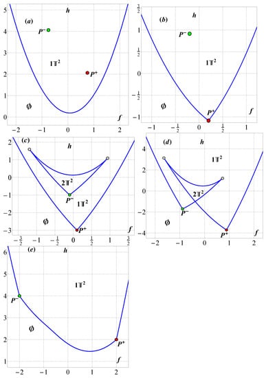
Figure 2.
The regions marked with the empty set correspond to the points of the -plane in which there are no possible motions. The points of bifurcation curves correspond to the critical values of the momentum map, which are the images of critical points of rank 1 (periodic motions). The regions of the -plane marked with or correspond to the values of the first integrals for which preimage of the momentum map contains 1 or 2 two-dimensional tori, respectively. Points and correspond to focus singularities of rank 0 (equilibrium points). Qualitatively different types of bifurcation diagrams (a–e) are determined by the constants and correspond to the regions shown in Figure 1.
We find, explicitly, the bracket at the point of the critical subsystem :
As expected, the degeneracy of the symplectic structure occurs at the points where the polynomial vanishes, i.e., at the cusp points of the bifurcation curve .
4. Stability of Critical Trajectories
As an application, we investigate the problem of the stability of critical trajectories (11). It is sufficient to determine the type (elliptic/hyperbolic) at any one of the points of the smooth branch of the curve given by the formula in (13).
The type of critical point of rank 1 in an integrable system with two degrees of freedom is calculated as follows. It is necessary to specify the first integral G, such that and in the neighborhood of this point. The point turns out to be fixed for the Hamiltonian field and it is possible to calculate the linearization of this field at a given point – the symplectic operator at the point . This operator will have two zero eigenvalues, the remaining multiplier of the characteristic polynomial has the form , where . At , we get a point of type “center” (the corresponding periodic solution has an elliptic type, is a stable periodic solution in phase space, the limit of a concentric family of two-dimensional regular tori), and at we get a point of type “saddle” (the corresponding periodic solution has a hyperbolic type, there are movements asymptotic to this solution lying on two-dimensional separatrix surfaces). As an integral of G, we can take the function
Here, the expressions and are defined by the Formula (12), and the parameter s defines a point on the bifurcation curve (13).
The coefficient for the characteristic polynomial has the explicit form
where is the polynomial is responsible for the cusp points of the bifurcation curve (13). Thus, where the polynomial has a negative sign, regular precessions will be unstable. In Figure 2c,d, this corresponds to the branch of the bifurcation curve between the cusp points. At the remaining points of the bifurcation curve, regular precessions have an elliptical type, which corresponds to the stability of regular precessions.
Note that the work [3] is devoted to the study of the stability of regular precessions of a Lagrange top with a vibrating suspension point. In the present paper, the study of the stability of regular precessions is carried out on the basis of determining the type of singularity and geometric presentation on the bifurcation diagram of the equilibrium point and periodic motion stability.
The most important advantages of the method used in this paper to study the Lagrange top with a vibrating suspension point are the geometric clarity of the form of presentation of the results and general methods for studying the phase topology of integrable Hamiltonian systems. Having constructed the image of the critical set, we obtain a partition of the parameter space of the system under study into areas, inside which the number of connected components of the level set of first integrals does not change, and the nature of the singularities of the Liouville foliation is determined by the eigenvalues of the linearization of the symplectic operator at singular points. The bifurcation diagram, in such a clear geometric way, contains information about the nature of the stability of equilibrium positions and periodic solutions. In contrast to this technique, when studying the stability of equilibrium positions or periodic motions using standard methods used, for example, in [1,2,3,4], there is a need to construct the Lyapunov function or study the normal form in the vicinity of the equilibrium position (periodic motion). Here, there is a finding which, in itself, is a non-trivial mathematical problem and the construction of the Lyapunov function or normal form is the central problem of stability theory. On the other hand, classical methods almost always answer the question about the type of stability of singular solutions, even when the system is not Liouville integrable or is not Hamiltonian at all. However, the method presented in the article gives an answer to the question of the stability of primarily Liouville integrable Hamiltonian systems. At the moment, this approach is generalized to nonholonomic systems and in the case of dissipative systems, the question of the possibility of generalizing it is currently open.
Finally, we should note the results of the publication [12] where the authors presented four generic types of bifurcation diagrams. In this paper, we present five different types of bifurcation diagrams. This fact is not a contradiction because the objects that are being classified are different. Lagrange top was studied in [12] as a system with three degrees of freedom with three-dimensional bifurcation diagrams, and there are four types. In the present paper, the reduction of the top to the body frame is studied, which is a system with two degrees of freedom and hence a two-dimensional bifurcation diagram, and there are five types. The objects are related in that planar slices of the bifurcation diagram in [12] give the bifurcation diagrams in this paper, but the number of topologically different planar slices can be larger than the number of topologically different three-dimensional diagrams.
Author Contributions
Conceptualization, P.E.R.; Investigation, P.E.R. and S.V.S. All authors have read and agreed to the published version of the manuscript.
Funding
This research was partially supported by the Russian Science Foundation, grant no. 19-71-30012 and the Russian Foundation for Basic Research, grant no. 20-01-00399.
Data Availability Statement
Not applicable.
Conflicts of Interest
The authors declare no conflict of interest.
References
- Markeev, A.P. On the theory of motion of a rigid body with a vibrating suspension. Dokl. Phys. 2009, 54, 392–396. [Google Scholar] [CrossRef]
- Markeev, A.P. The equations of the approximate theory of the motion of a rigid body with a vibrating suspension point. J. Appl. Math. Mech. 2011, 75, 132–139. [Google Scholar] [CrossRef]
- Markeev, A.P. On the motion of a heavy dynamically symmetric rigid body with vibrating suspension point. Mech. Solids 2012, 47, 373–379. [Google Scholar] [CrossRef]
- Kholostova, O.V. The dynamics of a Lagrange top with a vibrating suspension point. J. Appl. Math. Mech. 1999, 63, 741–750. [Google Scholar] [CrossRef]
- Bolsinov, A.V.; Borisov, A.V.; Mamaev, I.S. Topology and Stability of Integrable Systems. Russ. Math. Surv. 2010, 65, 259–318. [Google Scholar] [CrossRef]
- Kharlamov, M.P. Bifurcation diagrams of the Kowalevski top in two constant fields. Regul. Chaotic Dyn. 2005, 10, 381–398. [Google Scholar] [CrossRef]
- Kharlamov, M.P.; Ryabov, P.E. Topological atlas of the Kovalevskaya top in a double field. J. Math. Sci. 2017, 223, 775–809. [Google Scholar] [CrossRef]
- Kharlamov, M.P.; Ryabov, P.E.; Savushkin, A.Y. Topological Atlas of the Kowalevski-Sokolov top. Regul. Chaotic Dyn. 2016, 21, 24–65. [Google Scholar] [CrossRef]
- Kharlamov, M.P.; Ryabov, P.E.; Kharlamova, I.I. Topological Atlas of the Kovalevskaya-Yehia Gyrostat. J. Math. Sci. 2017, 227, 241–386. [Google Scholar] [CrossRef]
- Bolsinov, A.V.; Fomenko, A.T. Integrable Hamiltonian Systems. Geometry, Topology, Classification; Chapman & Hall/CRC: Boca Raton, FL, USA, 2004; 730p. [Google Scholar]
- Borisov, A.V.; Ryabov, P.E.; Sokolov, S.V. On the Existence of Focus Singularities in One Model of a Lagrange Top with a Vibrating Suspension Point. Dokl. Math. 2020, 102, 468–471. [Google Scholar] [CrossRef]
- Dawson, S.R.; Dullin, H.R.; Nguyen, D.M.H. The Harmonic Lagrange Top and the Confluent Heun Equation. Regul. Chaotic Dyn. 2022, 27, 443–459. [Google Scholar] [CrossRef]
Disclaimer/Publisher’s Note: The statements, opinions and data contained in all publications are solely those of the individual author(s) and contributor(s) and not of MDPI and/or the editor(s). MDPI and/or the editor(s) disclaim responsibility for any injury to people or property resulting from any ideas, methods, instructions or products referred to in the content. |
© 2023 by the authors. Licensee MDPI, Basel, Switzerland. This article is an open access article distributed under the terms and conditions of the Creative Commons Attribution (CC BY) license (https://creativecommons.org/licenses/by/4.0/).