Analysis of Industrial Product Sound by Applying Image Similarity Measures

Abstract

The sounds of certain industrial products (machines) carry important information about these products. Product classification or malfunction detection can be performed utilizing a product’s sound. In this regard, sound can be used as it is or it can be mapped to either features or images. The latter enables the implementation of recently achieved performance improvements with respect to image processing. In this paper, the sounds of seven industrial products are mapped into mel-spectrograms. The similarities of these images within the same class (machine type) and between classes, representing the intraclass and interclass similarities, respectively, are investigated. Three often-used image similarity measures are applied: Euclidean distance (ED), the Pearson correlation coefficient (PCC), and the structural similarity index (SSIM). These measures are mutually compared to analyze their behaviors in a particular use-case. According to the obtained results, the mel-spectrograms of five classes are similar, while two classes have unique properties manifested in considerably larger intraclass as opposed to interclass similarity. The applied image similarity measures lead to similar general results showing the same main trends, but there are differences among them as mutual relationship of similarity among classes. The differences between the images are more blurred when the SSIM is applied than using ED and the PCC.

1. Introduction

Image processing has attracted wide attention in the last several decades. This technique includes diverse tasks, among which image quality or degradation assessment, i.e., image similarity, stands out [1,2,3]. During this period of development, a number of algorithms for image comparison were developed [4]. Similarity, in general, represents the degree of mirroring with respect to the connection between two components—two images in the case of image similarity [5]. Such similarity plays a vital role in various areas, such as meteorology and climatology [6], medical diagnostics [7], autonomous driving, speech processing and sound analysis [8], etc. Specifically, image similarity analysis is applied for solving problems such as object detection and image matching [2,9,10], face recognition [5], image structure and texture analysis [9,11], image synthesis and reconstruction [12], object tracking [13], etc.

The assessment of image similarity is a rather demanding task that is solved by applying different approaches to image comparison. These approaches are based on specific image similarity metrics or measures, also denoted as distance functions or distortion measures, which quantify the degree of matching between two images [9]. Some of these measures include the use of the peak-signal-to-noise ratio (PSNR), Euclidean distance (ED), squared ED (L2 norm) and mean absolute error (MAE; L1 norm), the structural similarity index measure (SSIM), and the feature similarity index measure (FSIM) [1,2,3,5,10,13,14]. Some of these measures are simple low-level measures, e.g., the L1 and L2 norms (distances), with limited ability to extract the high-level meaning of an image, such as semantic content-based objects, e.g., people, flowers, etc. [9]. On the other hand, some other measures, such as measures based on intensity probability distribution (joint and marginal entropies), are rather complex [15]. The requirements regarding the performance of the image similarity measures depend on the particular application. So, in image recognition, it is desirable to use a more shift- and rotation-robust measure, while in registration and tracking it is desirable to use a measure showing better localization and noise tolerance [16].

Besides image similarity belonging to two-dimensional (2D) similarity, one-dimensional (1D) similarity, e.g., signal similarity, has an essential role in diverse applications such as signal detection and pattern recognition. Measures often used to quantify 1D similarity include cosine similarity, angular similarity, Tanimoto similarity, and the Pearson correlation coefficient (PCC) [5].

Recently, sound- (audio) and vibration-based classification, recognition, and detection (CRD) methods have become more widespread. These methods can be employed in a number of applications, such as the prediction of the remaining useful life of a bearing [17], the detection of faults in a turbofan engine, the monitoring of gear units, the identification of damaged bearings in highly sophisticated engines such as aircraft engines [18], and the autonomous acoustic monitoring of processes and events within a manufacturing facility [19]. Compared with the image CRD methods, which constitute a heavily researched topic, audio CRD methods are significantly less mature [20]. In audio CRD methods, three general approaches can be identified: one based on hand-crafted features, the image-based approach, and the raw audio signal approach. The second approach has been widely accepted, especially after the rapid development of deep neural networks (DNNs) or, more specifically, convolutional neural networks (CNNs) and their increased capabilities as well as the availability of processing units [8]. In this way, the performance improvement from image processing can potentially be applied in audio signals, although the high performance of DNNs or CNNs is still not reached in the audio field [20].

There are various visual representations of audio signals; however, a critical review of the related signal representation techniques is missing in the literature [21]. The most common form of the visual representation of audio is provided through frequency spectrum variation in time, such as in a spectrogram [8,20,21]. A classical, full-resolution spectrogram brings the advantage that some unique properties of an audio signal will be revealed, but a large number of points will increase the computational cost of a CNN. This can be overcome by using frequency filter-banks, such as moving average and mel-filters, which can be employed to calculate the energy in particular frequency bands to reduce the number of points in the frequency domain [21].

Since audio and vibration signals have unique patterns when mapped into an adequate image, the methods used in image processing, including image similarity analysis, can be applied to them as well. Thus, an image texture analysis-oriented gray-level co-occurrence matrix is utilized for sound recognition in audio surveillance, where central moments extracted from the spectrogram image are used as features [22]. Unsupervised similarity analysis (cosine similarity) in combination with a CNN is employed to identify and track industrial processes using the acoustic signatures of spectrograms [19]. The power spectrum of mel-frequency cepstral coefficients (MFCC) is combined with the spectrogram image for the real-time monitoring of empathy in advertisements [23]. The quality of audio signals after compression is assessed by means of a structural similarity measure such as the mean structural similarity (MSSIM), which is applied to the fixed time-domain frames of an audio sequence and to 2D time-frequency maps [24]. The condition monitoring and fault diagnosis of a bearing system are carried out by comparing the spectral images of normal vibration data with the tested data using either SSIM, as performed in [25], or by using PSNR, as performed in [18]. In other studies, the fault diagnosis of bearings is also performed by using the spectrogram and spectrum of vibration data, as stated in [18].

A number of presented studies and use-cases realized in practice have shown significant capabilities with respect to using sound for different tasks, such as classifying industrial products or detecting product malfunctions. In order to apply the performance gain from image processing, a sound is first mapped into adequate images, and then these images are used for further processing, as executed in DNN or CNN classifiers. Currently, there is no standardized method for mapping sound into an image (instead, different alternatives are applied) and assessing the information provided by the image. Therefore, this research aims to conduct such an assessment using three image similarity measures: ED, PCC, and SSIM. More precisely, we examine whether one of the commonly employed image representations of sound (the mel-spectrogram) contains sufficient descriptive information in order to distinguish between classes by estimating image similarity. The image similarity measures utilized herein are those often used in practice (see, for example, [4,7,11,26,27]), which are related to different aspects of image similarity, namely, the distance-related, correlative (linear relationship), and structural features of images. Moreover, the aim is also to provide information concerning the value of these similarity measures with respect to estimating the similarity of images with specific properties compared to natural images.

The research is carried out by incorporating the sounds of industrial products belonging to seven categories (types): fan, gearbox, pump, slide rail (slider), toy-car (also denoted as ToyCar), toy-train (also denoted as ToyTrain), and valve. These sounds are available as datasets within the “Detection and classification of acoustic scenes and events” (DCASE) 2021 challenge [28,29,30]. The sounds are first mapped into the mel-spectrogram images. Then, the mentioned three image similarity measures are calculated for all these images, and they are used to analyze the sounds of the industrial products by applying the image-processing approach. The analysis includes the usage of similarity matrices and heat maps; additionally, a statistical analysis is carried out. The focus is on the intraclass and interclass similarities in order to show how similar the sounds belonging to the same class and different classes are.

The novelty of this research can be summarized in the following main contributions:

• Assessed information contained in mel-spectrograms, which were obtained by mapping the sounds of industrial products from the perspective of the image similarity within and between the classes, that is, whether a given image often applied in practice is able to describe the distinctive content of a given sound;
• Analyzed intraclass and interclass similarities at the level of mel-spectrogram images, thereby providing a basis for the development of a parametric classifier;
• Evaluated performance of three often-used image similarity measures for estimating the similarity of images with properties that are different from natural images, such as properties concerning different meanings of axes (time and frequency, i.e., width and height), image transparency, and non-locally distributed objects (harmonics) [31].

This paper is organized as follows: Section 2 describes the image similarity measures used in this research. The methodology of investigation, including the datasets used, the audio signal processing employed, and the calculation of similarity measures, is explained in Section 3. The results are presented in Section 4, which is divided into three subsections describing the analysis at different levels. Section 5 presents a discussion of the results and their comparison with those from the literature, while conclusions and directions for future research are summarized in Section 6.

2. Image Similarity Measures Used in This Research

2.1. Image Similarity in Literature and Practice

In practice, a number of measures have been used to evaluate image similarity and quality. These measures range from traditional measures that assess image similarity on a point-by-point basis, such as the mean square error (MSE) and PSNR, to more sophisticated measures such as perceptual quality measures or metrics [11]. The former are commonly inadequately correlated with subjective evaluations performed by human observers [7] and do not always provide convincing results [26]. The mentioned MSE and MAE are sensitive to both an image’s relative position and its content [32]. Historically, the use of the MSE, together with cross-correlation, has constituted the most popular approach used to measure image similarity [32].

There are also some other measures that belong to the classes of either statistical methods (calculating image statistics) or spectral methods (utilizing either Fourier transform or sub-band decomposition), as defined in [11]. On the other hand, some measures focus on structural similarity, incorporating the high-level properties of the human visual system. The popularity of using simple point-by-point difference measures has diminished in favor of measures based on information theory, such as mutual information (MI), which constitutes a general measure of information content that provides more flexibility [32]. Unfortunately, these advantages come with increased computational costs.

Three image similarity measures are used herin to estimate the mel-spectrograms’ similarity: ED, PCC, and SSIM. These measures are selected in such a way as to have different behaviors regarding several criteria. They include the simplicity of implementation, computational efficiency, sensitivity to outliers, spatial pixel distribution, the estimation of absolute (global) similarity or perceived (subjective) similarity, and the type of similarity assessment (e.g., pixel-based or structure-based). Moreover, the measures utilized in this research are those that are frequently used in many presented studies. Other similarity measures and methods can also be applied for the stated purpose, such as some of those mentioned above, recurrence quantification analysis [33], or various machine learning approaches [31].

2.2. Euclidean Distance

The oldest and simplest measure for evaluating image similarity is the MSE [26,34,35]. It can be calculated from 1D or 2D data, wherein the former is applied as follows:

$$MSE=\frac{1}{N}{\displaystyle \sum _{i=1}^N{\left(x_i-y_i\right)}^2},$$

(1)

where x_i and y_i are 1D data (e.g., two images represented as 1D vectors) and N is the number of pixels of these images. The MAE is calculated in a similar way, where the squared difference is replaced by the absolute value of difference. Both the MSE and MAE are sensitive to outliers, although the MAE is more sensitive [34]. These two measures can become more robust by replacing the summation in Equation (1) by an α-trimmed summation (see [34]).

Unfortunately, the MSE does not consider either the arrangements of the image pixels (spatial distribution) or their correlation [35]. Moreover, all image pixels have the same importance with respect to calculating the MSE. In addition, the spatial average value of the compared images has a strong effect on the MSE [6]. These facts represent important disadvantages of the MSE in particular tasks such as image quality estimation, where, for example, the arrangement and structure of pixels directly affect the images’ quality since the images are highly structured.

The MSE can also be calculated from 2D data, as follows:

$$MS{E}_{2D}=\frac{1}{W\cdot H}{\displaystyle \sum _{i=1}^W{\displaystyle \sum _{j=1}^H{\left(x_{i,j}-y_{i,j}\right)}^2}},$$

(2)

where W and H indicate the number of rows and columns of 2D data, e.g., images. This measure provides an estimation of absolute similarity, and it is computationally efficient [32].

A measure that is closely related to the MSE is ED [27], which quantifies the distance between two corresponding points of two 1D vectors, x and y, in Euclidean space as

$$ED=\sqrt{{\displaystyle \sum _{i=1}^N{\left(x_i-y_i\right)}^2}}=\sqrt{N\cdot MSE}.$$

(3)

Compared images are more alike if the ED value is smaller. This measure belongs to the LP (P is the norm) family of similarity metrics (measures) or the Minkowski metric; more precisely, the ED is the L2 metric also called sum of square error [9]. The ED is used in various tasks, such as measuring the distance between two spectral images to predict the remaining useful life of bearings [17] and predicting images outside of the field of view, that is, widening the field of view [10].

2.3. Pearson Correlation Coefficient

One of the most often-used measures of correlation is the PCC, which reflects the degree of the linear relationship between two variables [36]. The PCC is a statistical index, and can be calculated as follows [5,37]:

$$PCC=\frac{{\displaystyle \sum _{i=1}^N\left(x_i-{\mu }_x\right)\left(y_i-{\mu }_y\right)}}{{\displaystyle \sum _{i=1}^N{\left(x_i-{\mu }_x\right)}^2}{\displaystyle \sum _{i=1}^N{\left(y_i-{\mu }_y\right)}^2}}=\frac{{\sigma }_{xy}}{{\sigma }_x{\sigma }_y},$$

(4)

where x_i and y_i are the values of the i-th pixel in images x and y, respectively, which are transformed into 1D vectors having the length N; μ_x and μ_y are the mean values of images x and y, respectively; σ_XY is the covariance between x and y; and σ_X and σ_Y are the standard deviations of x and y, respectively. The PCC defined in Equation (4) is also known as the zero-mean cross correlation coefficient.

The PCC ranges from +1 to −1, where these values are related to a perfect positive (the highest similarity or perfect match) and a negative linear relationship, respectively [6,36]. A PCC value of 0 indicates that there is no linear relationship between the two variables. The mentioned two properties of the PCC—the fixed range of values [−1, 1] and the linear relationship between images—represent two crucial advantages of this measure [32].

The PCC is identified as a scalar measurement of global similarity between compared images. This measure is often used for template matching and pattern recognition [32]. It is less sensitive to changes in illumination than the MSE and MAE [34]. The PCC should be used when changes in illumination may be approximated with a linear transformation. When this is not the case, a better option would be either MI or another ordinal similarity measure [34]. The PCC measure can be made robust against outliers by applying a modification proposed in [34].

2.4. Structural Similarity

Natural images possess an important property, namely, they are highly structured, i.e., there is a high degree of correlation between spatially close pixels [16]. This can be used to extract meaningful information about the structure of objects in a visual scene. On the other hand, the structural similarity between images can remarkably approximate the perceived image similarity [35]. The most popular measure related to image structure is the SSIM index.

When the SSIM index is used to assess image similarity (or more precisely, the structural similarity between two images), this task is divided into three sub-tasks: the comparison of luminance (brightness), contrast, and structure. In this comparison, the local statistics and SSIM index are calculated within the local window. In other words, the SSIM is obtained for each overlapped image window via the use of a pixel-by-pixel sliding window. This is an advantage of the SSIM measure since the statistical properties of an image are not the same for every part of the image [35]. In addition, the calculation of the SSIM over segments of data is advantageous from a complexity standpoint, and it also allows one to weigh the segments unequally [24].

Let p and r be local square windows (patches) of the images x and y, respectively, located at the same spatial positions in both images. The mentioned luminance, contrast, and structure are calculated as follows:

$$l\left(p,r\right)=\left(2{\mu }_p{\mu }_r+C_1\right)/\left({\mu }_p^2+{\mu }_r^2+C_1\right)$$

(5)

$$c\left(p,r\right)=\left(2{\sigma }_p{\sigma }_r+C_2\right)/\left({\sigma }_p^2+{\sigma }_r^2+C_2\right)$$

(6)

$$s\left(p,r\right)=\left({\sigma }_{pr}+C_3\right)/\left({\sigma }_p{\sigma }_r+C_3\right),$$

(7)

where μ _p and μ _r represent the average pixel values in the local windows p and r, respectively; σ_p and σ_r represent the standard deviation of the pixel values in these local windows; σ_pr represents the covariance (cross-correlation) of the p and r windows; and C₁, C₂, and C₃ are constants introduced to avoid instabilities when the sums in the denominators of the previous three equations are close to zero [2,3,6,7,10,14]. The size of the local window can be 11 × 11, as used in [12]. For the application of the SSIM to audio signals, the comparison of luminance is not of particular interest since longer audio sequences have a mean of zero [24].

In this way, the luminance and contrast data are separated from the structural information, but all of them are combined to assess the similarity of the images. Here, the structural information is related to the shape of the objects [35]. Apart from the constant C₃, the structure term represents the cross-correlation coefficient of the two local windows [11]. The luminance and contrast terms scaled by the mean and variance values, respectively, have values in the interval between 0 and 1, while the structure term has a value in the interval between −1 and 1. The SSIM measure incorporates implicit contrast masking.

The SSIM index is obtained by combining these three terms as follows:

$$SSIM\left(p,r\right)={\left[l\left(p,r\right)\right]}^{\alpha }{\left[c\left(p,r\right)\right]}^{\beta }{\left[c\left(p,r\right)\right]}^{\gamma }.$$

(8)

The variables α, β, and γ are the parameters defining the relative importance of each component, often set to 1. The SSIM can have values between 0 and 1, where the former means that the images are completely different, and the latter means that the images are identical. The final SSIM index (across all spatial locations) used for the evaluation of global image similarity is obtained as the mean of the SSIM in the local windows. It is stated in the literature that the SSIM objectively predicts the subjective image quality rating [11,12], except in noisy and blurred images as well as in images close to recognition thresholds [7].

The SSIM index shifts image similarity and quality assessment from a pixel-based (point-to-point) to a structure-based stage [38]. The SSIM and SSIM-based measures are often used in the image-processing field. Thus, the SSIM has been used in many studies as an unofficial standard for assessing image quality when a reference image is available [4], e.g., in image recognition.

3. Methodology

3.1. Dataset

Sound samples (audio signals) used in this research were taken from the task 2 “Unsupervised anomalous sound detection for machine condition monitoring under domain shifted conditions” of the DCASE 2021 challenge [28]. The dataset available for the mentioned challenge was generated from two datasets: MIMII DUE [29] and TOYADMOS2 [30]. The obtained dataset consists of normal and anomalous (abnormal) operating sounds of seven types of machines (industrial products): fan, gearbox, pump, slider, toy-car, toy-train, and valve. Sounds from all seven machine types were recorded in the same way, thereby making the samples uniform and easy to compare in further analysis. This dataset was generated to investigate malfunctioning industrial machines and perform inspections with domain shifts (between the source and target domain) due to changes in operational and environmental conditions [29]. The source domain is related to the original condition in which there were a sufficient number of sound samples for training, while the target condition is related to the changed condition in which only a few sound samples were available for training. Differences in the source and the target domain (domain shifts) include those regarding operating speed, machine load, environmental noise, heating temperature, SNR, etc. [29], that is, the use of the same machine type but with different machine models and part configurations, microphone arrangements, etc. [30]. The described dataset was designed for anomalous sound detection, that is, the automatic detection of machine malfunctions.

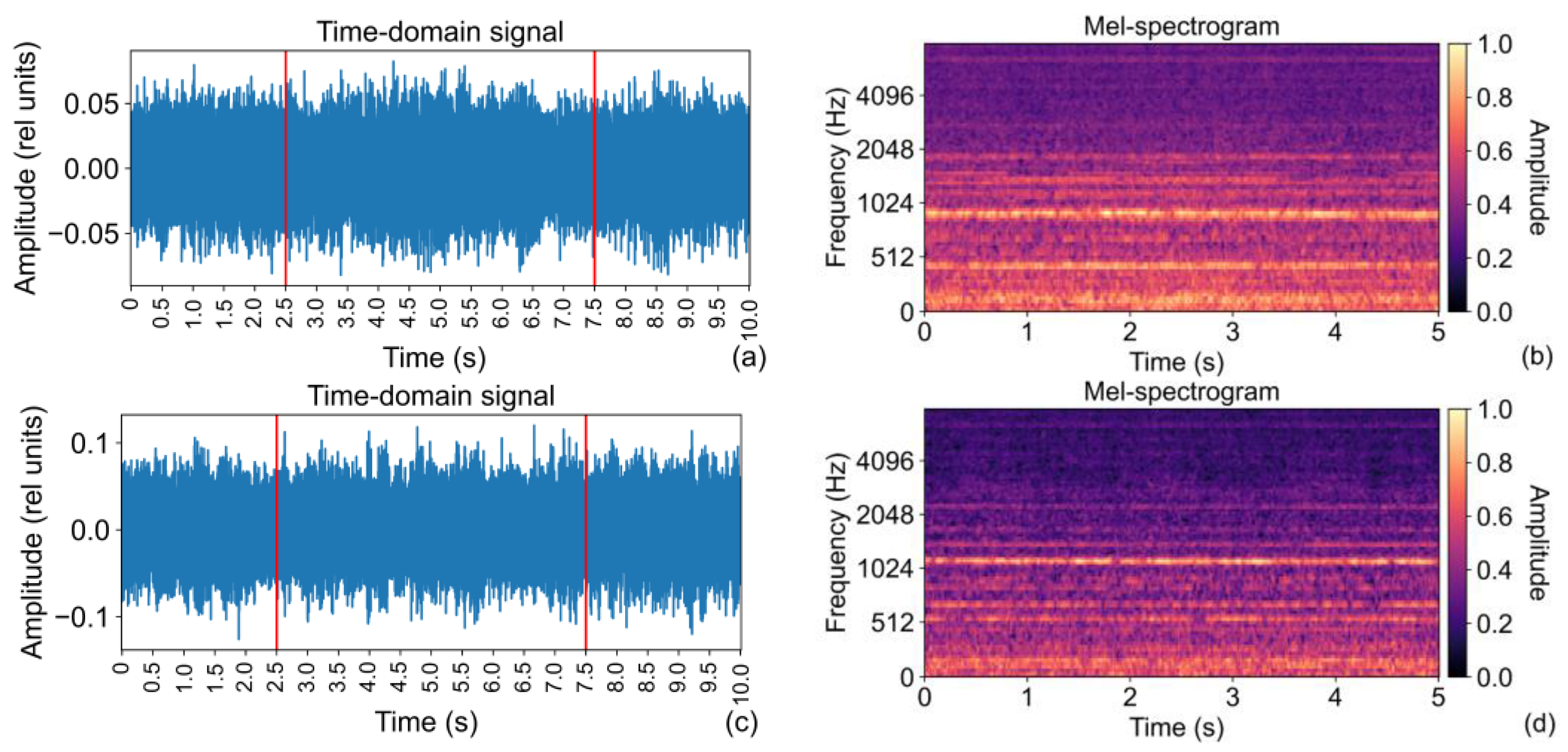
The sound samples represent single-channel (mono), 16-bit recordings of sounds of the mentioned machines (thus having a resolution of 2¹⁶ = 65,536) with a duration of 10 s saved in the “wav” format. These samples contain the sound of a target machine, but also sounds of associated equipment and environmental sounds. The sampling frequency of the recorded signals is 16 kHz. The machine sounds were recorded utilizing the microphone array Tamago-03, where only an audio signal from the first microphone of the array was used [29], that is, through five to eight microphones [30]. The recordings were performed either in an anechoic chamber, ordinary rooms, or a sound insulation booth. Background noise from different factories was recorded separately, and it was mixed with machine sounds in the postprocessing phase. Details can be found in [29,30]. Two illustrative examples of the sound samples in the time and frequency domain are presented in Figure 1.

All recorded sound samples are split into three datasets: development, additional training, and evaluation datasets. The development dataset consists of three sections with 1003 sound samples for each machine, where each section roughly corresponds to a single product. In each section, there are only normal operating sound samples from two domains (1000 samples from the source domain, and 3 samples from the target domain), with different conditions such as operating speed and environmental noise. Therefore, 3009 sound samples are available per machine. For the research presented herein, this development dataset—incorporating sound samples from both source and target domains as well as normal operating mode—is used, and it is denoted as a full dataset. A smaller dataset, called the extracted dataset in this study, is generated in the same way as the full dataset, but by taking only 300 sound samples for each machine. In this extracted dataset, only the sound samples from the same section are included; therefore, they are generated roughly by the same product. Some analyses are carried out using this extracted dataset.

3.2. Audio Signal Processing

The sound signals with a duration of 10 s are initially preprocessed by extracting the 5 s long mid part of every signal, as illustrated in Figure 1a, representing the only modification of the original sound samples. In this way, the transient effects that could be present in the beginning and at the end of the signals are eliminated. Since the original sound signals show rather stationary behavior, shortening the signals does not remove any vital information; instead, it enables one to halve the size of mel-spectrograms in the time domain. Each such preprocessed (i.e., shortened) signal is mapped into a mel-spectrogram by applying a pipeline of operations. These operations include segmenting the sound signals into segments or frames, transforming each of these time frames into their frequency domain counterparts via the fast Fourier transform (FFT), filtering the obtained frequency representations using the mel-filter bank of triangular filters, and calculating the equivalent energy in the mel-bands. The width (frequency band) of mel-filters increases with frequency, but these bands are equally spaced on the mel-scale.

Mel-spectrogram is often used for mapping audio and acoustic signals into an image that is applied as an input in different classification and detection tasks based on DNNs, especially CNNs. Mel-scale is a non-linear frequency scale that matches human perceptual behavior; that is, it resembles the way in which humans perceive sound. In a mel-spectrogram, the resolution on the frequency axis is reduced compared to a classical (full-resolution) spectrogram. Here, the number of frequency bins is equal to the number of mel-bands, which is significantly smaller than the number of frequency bins in a classical spectrogram. Typically, this number of mel-bands is either 96 or 128. In this research, the number of mel-bands is 96, while the frame size is 1024 samples, and the step size (overlap between consecutive frames) is 256 samples. In this way, the mel-spectrogram has a size of 96 by 313, where 313 represents the number of frames.

For the calculation of some similarity measures such as ED and PCC, the mel-spectrogram images in the form of matrices are converted into arrays by concatenating the columns. These arrays are used as input for the ED and PCC calculation. On the other hand, the SSIM index is calculated using solely the generated mel-spectrograms themselves.

3.3. Calculation and Analysis of Image Similarity Measures

Similarity of images (mel-spectrograms in this case) is analyzed using the three similarity measures described in Section 2: ED, PCC, and SSIM. The ED and PCC are calculated by applying Equations (3) and (4), respectively, while the SSIM is calculated by applying Equations (5)–(8). The whole processing procedure including the audio signal’s processing as well as calculation and analysis of image similarity measures is performed in the Python programming language using the following modules and libraries: sys, os, inspect, matplotlib, soundfile, numpy, scipy, librosa, tensorflow, pandas, seaborn, skimage, and sklearn.

In order to obtain the similarity measures within the same class (the same industrial product or machine type, e.g., fan), i.e., the intraclass similarity, this measure is calculated for all possible combinations (pairs) of images belonging to that particular class (product). Since the order of images (i.e., which is the first and which is the second) is irrelevant with respect to the calculation of the three similarity measures used herein, all combinations without permutations are included in the analysis. To investigate the interclass similarity, the three selected similarity measures are calculated such that the first image is taken from one class while the second image is taken from another class. All combinations (pairs) of images without permutations are included in the calculations. In this way, a matrix for every particular class and image similarity measure is generated for intraclass similarity, while the number of such matrices for interclass similarity is six for each of the classes and similarity measures.

The generated intraclass and interclass similarity matrices are further investigated by generating the heat maps and applying statistical analysis. Thus, common statistical quantities—mean, minimum, maximum, median, and standard deviation (SD)—are calculated from the generated matrices. These values are used to carry out mutual comparisons among the three similarity measures chosen to be investigated within this research.

4. Results

Using the described procedure, three image similarity measures (ED, PCC, and SSIM) were calculated for a large number of pairs of samples, that is, the mel-spectrograms of the machines belonging to the stated seven classes. Since all the classes have either 3009 samples (the full dataset) or 300 samples (the extracted dataset), the similarity values were arranged in square matrices with dimensions of 3009 × 3009 or 300 × 300. As the order of the samples does not affect the obtained value of any of these three similarity measures, the mentioned matrices are symmetrical around the main diagonal. Moving along any of rows or columns of these matrices, the similarity values of a particular sample (machine) with all other compared samples either from the same class (intraclass similarity) or from another class (interclass similarity) are given. Since the values on the main diagonal are related to the self-similarity of each sample, these values are either 0 for ED or 1 for PCC and SSIM.

The results regarding intraclass similarity are presented in 21 matrices for the full dataset and the same number of matrices for the extracted dataset. Among these, each similarity measure has seven matrices (one for each machine type/class) for each dataset. The interclass similarity is presented in more matrices than the intraclass similarity. Thus, there are 3 × 21 matrices for each dataset given that all the combinations of the samples but not their permutations were considered.

The obtained similarity values are analyzed from different perspectives and in both directions from detailed to more general analysis and vice versa. Here, the results are presented in a direction from a general to a more detailed analysis.

4.1. Analysis at the Level of Statistical Quantities of Image Similarity Measures

For each of the mentioned image similarity matrices, statistical quantities such as the mean, minimum, maximum, median, and SD are calculated and presented in a tabular format.

Table 1. Statistical quantities of intraclass similarity measures (ED, PCC, and SSIM) obtained using the full dataset.

Machine Type	Measure	Mean	Minimum	Maximum	Median	SD
Fan	ED PCC SSIM	23.66 0.76 0.38	10.46 −0.42 0.09	69.52 0.94 0.64	23.11 0.77 0.37	6.77 0.12 0.07
Slider	ED PCC SSIM	25.77 0.71 0.35	11.98 −0.33 0.09	73.53 0.93 0.62	25.09 0.72 0.34	6.76 0.14 0.07
Gearbox	ED PCC SSIM	24.85 0.72 0.36	11.69 −0.38 0.10	76.46 0.93 0.64	24.19 0.73 0.36	7.10 0.14 0.07
Pump	ED PCC SSIM	24.57 0.74 0.36	11.17 −0.44 0.09	71.44 0.95 0.63	23.78 0.75 0.35	6.59 0.13 0.07
Valve	ED PCC SSIM	25.07 0.74 0.36	11.98 −0.23 0.07	65.42 0.94 0.63	24.26 0.74 0.36	6.74 0.12 0.07
Toy-car	ED PCC SSIM	15.57 0.89 0.57	3.03 0.36 0.31	44.26 1.0 0.98	14.83 0.90 0.58	3.21 0.04 0.04
Toy-train	ED PCC SSIM	23.98 0.65 0.43	5.58 0.05 0.23	51.49 0.99 0.93	23.62 0.66 0.42	5.28 0.14 0.06

presents a summary of these statistical quantities in the case of intraclass similarity for the full dataset and all three measures (excluding self-similarity). It can be seen that the range of the values as well as the direction of the values’ increase/decrease for ED is not the same as for PCC and SSIM, as described above. Thus, a smaller similarity value in ED indicates more similar images, while the situation is opposite with respect to the PCC and SSIM. The range of values (from minimal to maximal) for all three measures is rather wide even though all the compared samples belong to the same classes. It is worth mentioning that the PCC can have negative values, which can be treated in different ways, e.g., to take them as they are or to take them as zeros. For the analysis presented here, they are treated as negative values. Since there are not many of such negative PCC values, they do not significantly affect the results of the performed statistical analysis. On the other hand, the SD of PCC is between 0.12 and 0.14 and the SD of SSIM is between 0.06 and 0.07 for all classes except for the toy-car, which is 0.04 for both PCC and SSIM. This indicates that the spread of the similarity values from the mean is not that large.

The minimum values of ED are in the range from 10.46 to 11.98 for five classes (fan, slider, gearbox, pump, and valve), denoted here as a group of five classes, while they are smaller for two classes, namely, toy-car and toy-train, with the values of 3.03 and 5.58, respectively. The trend is opposite with respect to the maximum values for PCC and SSIM, wherein they are smaller for the group of five classes and larger (close to 1) for the toy-car and toy-train classes.

The statistical quantities in the case of interclass similarity represented by the PCC measure (excluding self-similarity) for the full dataset are given in

Table 2. Statistical quantities of interclass similarity obtained using PCC measure calculated from the full dataset.

Machine-Type Pair	Mean	Minimum	Maximum	Median	SD
Fan–Slider	0.74	−0.41	0.93	0.74	0.13
Fan–Gearbox	0.74	−0.42	0.96	0.75	0.13
Fan–Pump	0.75	−0.44	0.94	0.76	0.13
Fan–Valve	0.75	−0.41	0.94	0.75	0.12
Fan–Toy-car	0.78	−0.44	0.90	0.80	0.09
Fan–Toy-train	0.33	−0.51	0.82	0.35	0.21
Slider–Gearbox	0.72	−0.35	0.93	0.72	0.14
Slider–Pump	0.73	−0.42	0.93	0.73	0.13
Slider–Valve	0.73	−0.34	0.93	0.73	0.13
Slider–Toy-car	0.75	−0.30	0.90	0.77	0.10
Slider–Toy-train	0.30	−0.48	0.79	0.32	0.21
Gearbox–Pump	0.73	−0.42	0.94	0.74	0.14
Gearbox–Valve	0.73	−0.34	0.93	0.73	0.13
Gearbox–Toy-car	0.75	−0.32	0.90	0.77	0.11
Gearbox–Toy-train	0.29	−0.55	0.80	0.31	0.21
Pump–Valve	0.74	−0.43	0.94	0.74	0.12
Pump–Toy-car	0.76	−0.51	0.91	0.78	0.10
Pump–Toy-train	0.29	−0.58	0.80	0.31	0.21
Valve–Toy-car	0.76	−0.17	0.90	0.78	0.09
Valve–Toy-train	0.30	−0.43	0.80	0.32	0.21
Toy car–Toy-train	0.35	−0.34	0.80	0.39	0.23

. All possible combinations of machine types (classes), but not permutations, are included. The minimum values of the PCC in this format do not provide valuable information due to the presence of negative PCC values. The maximum values are rather large; they are in the range from 0.79 to 0.96. For comparison, the maximal PCC values in the intraclass similarity are between 0.93 and 0.95 for the group of five classes, and 0.99 for the toy-train and 1.0 for the toy-car classes. The SDs for the majority of the pairs of classes are close to 0.13, while smaller values (about 0.09) were obtained for the pairing of toy-car and any other class, and larger values (about 0.21) were obtained for the pairing of toy-train and any other class.

As presented in Table 2 for the PCC, the statistical quantities of the interclass SSIM similarity for the full dataset are summarized in

Table 3. Statistical quantities of interclass similarity obtained using SSIM measure calculated from the full dataset.

Machine Type Pair	Mean	Minimum	Maximum	Median	SD
Fan–Slider	0.35	0.06	0.61	0.35	0.07
Fan–Gearbox	0.36	0.08	0.63	0.35	0.07
Fan–Pump	0.36	0.08	0.64	0.35	0.07
Fan–Valve	0.37	0.07	0.66	0.36	0.07
Fan–Toy-car	0.38	0.12	0.53	0.39	0.05
Fan–Toy-train	0.31	0.04	0.50	0.32	0.06
Slider–Gearbox	0.35	0.09	0.62	0.34	0.06
Slider–Pump	0.35	0.10	0.62	0.34	0.07
Slider–Valve	0.35	0.08	0.61	0.34	0.07
Slider–Toy-car	0.37	0.12	0.50	0.38	0.05
Slider–Toy-train	0.30	0.03	0.47	0.31	0.06
Gearbox–Pump	0.35	0.10	0.63	0.34	0.07
Gearbox–Valve	0.36	0.08	0.63	0.35	0.07
Gearbox–Toy-car	0.37	0.12	0.51	0.37	0.05
Gearbox–Toy-train	0.31	0.04	0.49	0.31	0.06
Pump–Valve	0.36	0.07	0.64	0.35	0.07
Pump–Toy-car	0.38	0.11	0.53	0.39	0.05
Pump–Toy-train	0.30	0.04	0.49	0.30	0.06
Valve–Toy-car	0.38	0.11	0.51	0.39	0.06
Valve–Toy-train	0.31	0.03	0.48	0.32	0.06
Toy-car–Toy-train	0.35	0.18	0.54	0.36	0.04

. Here, the minimal values of the SSIM are positive, and they are rather small (between 0.04 and 0.18) for all pairs of classes. The maximal values of the SSIM are in the range from 0.48 to 0.66. Regarding the intraclass similarity, the maximal values for the group of five classes are between 0.62 and 0.64, and very close to 1 for other two classes (toy-car and toy-train). The SD values are in a rather narrow range between 0.05 and 0.07. For the pairing of toy-car and any other class, the maximal values are slightly smaller and the median values are slightly greater than for pairs of any other two classes except those wherein toy-train is one of the classes. Pairs wherein one of the classes is toy-train have smaller maximal and median values than other pairs wherein toy-train is replaced by another class. Such an observation is valid for both the PCC (Table 2) and SSIM (Table 3).

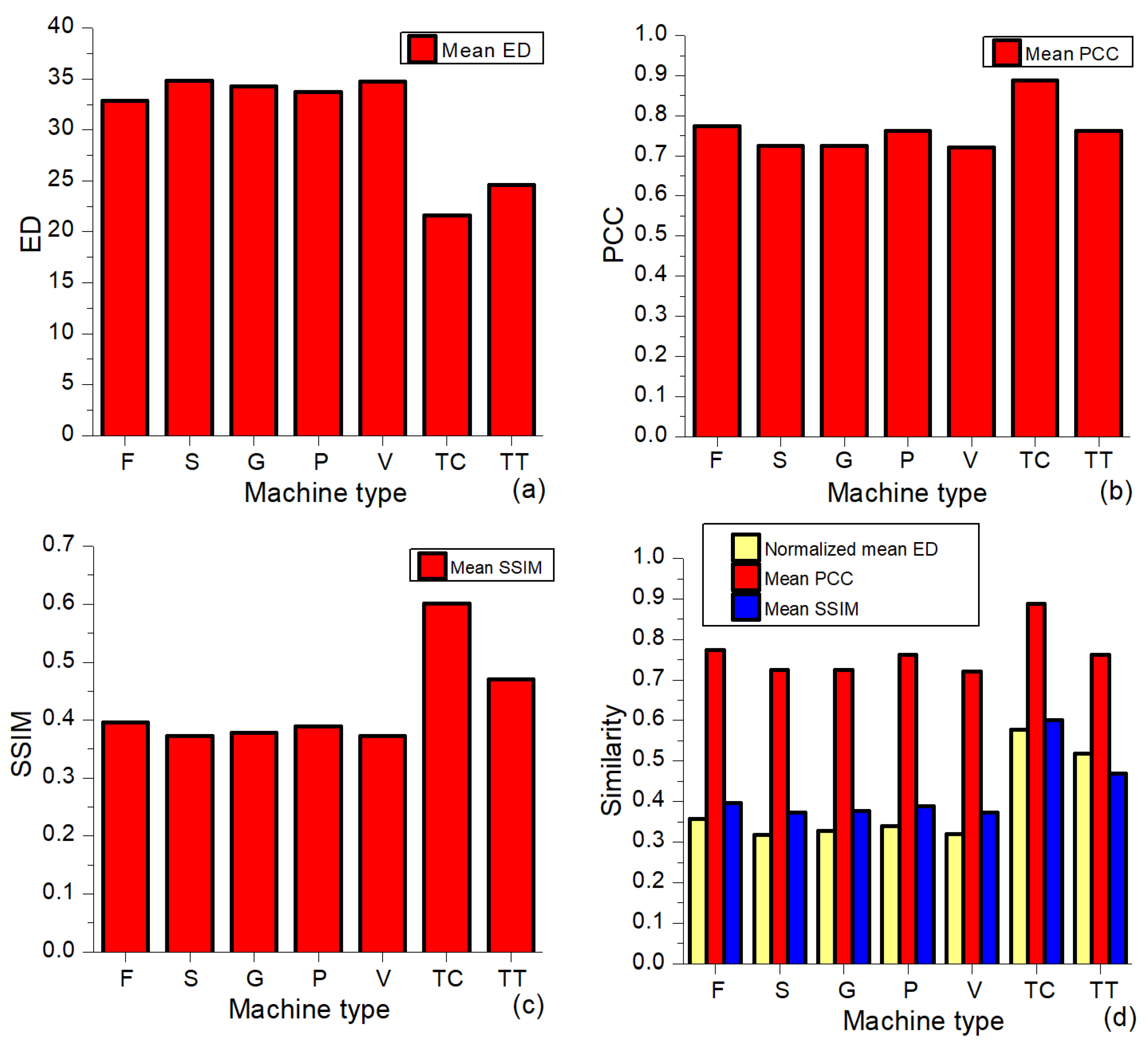
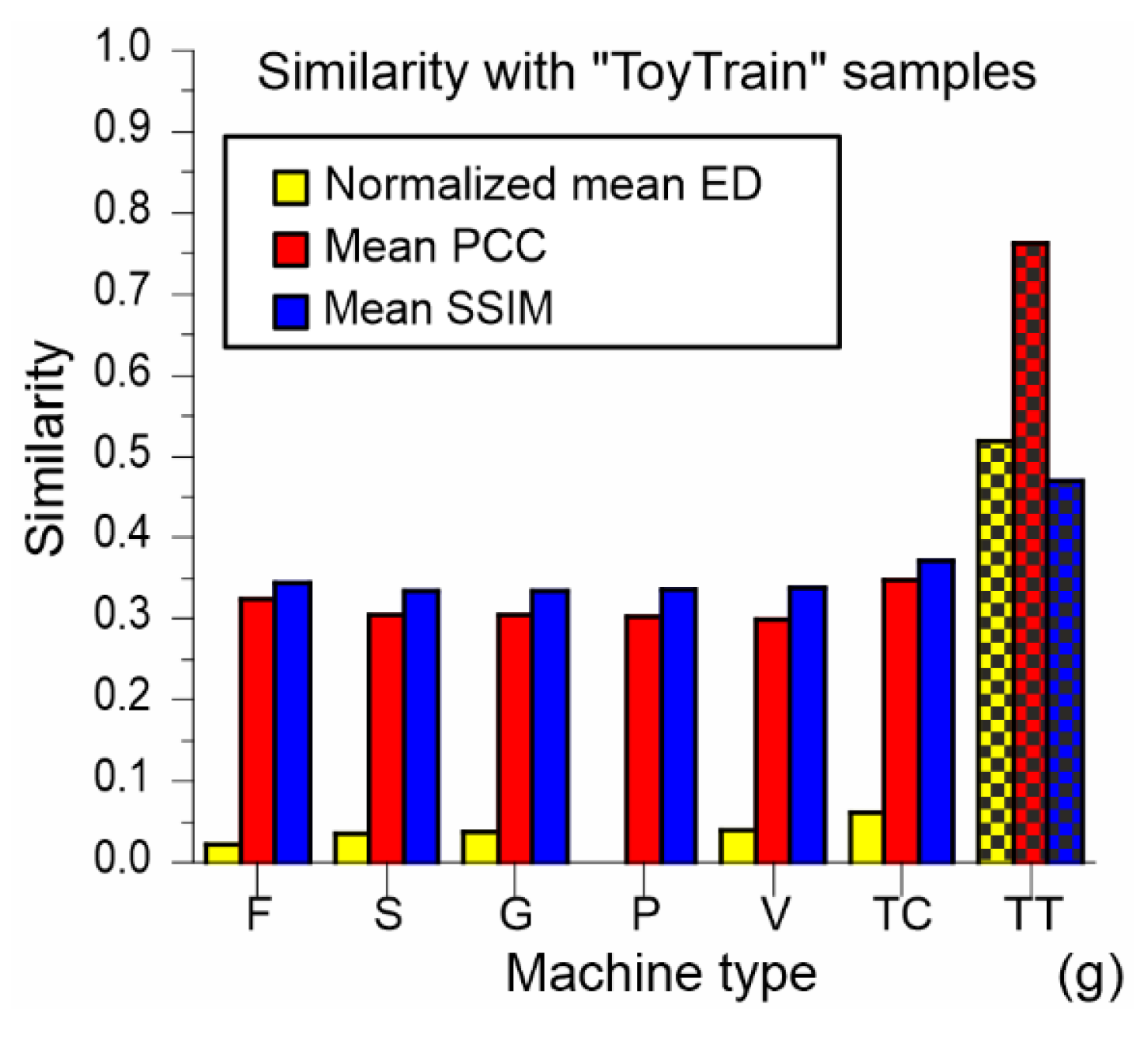
The statistical mean values of the similarity measures are given in Table 1, Table 2 and Table 3. In order to enable better visibility of the main trends, the obtained numerical values are also presented as bar plots. The mean values of the intraclass similarity for all three measures (ED, PCC, and SSIM) and the full dataset (see Table 1) are shown in Figure 2. The abbreviations used for the machine types (classes) in this figure are also applied in other figures. Comparing the presented values for the analyzed seven classes, it can be concluded that the intraclass similarity is the largest for the toy-car, followed by the toy-train and then other classes with very similar mean values. This observation is the most visible with respect to SSIM and ED, while the intraclass similarity of the toy-train class with respect to the PCC is similar to other classes, except that the toy-car class has the largest mean similarity value.

From Table 1 and Figure 2a–c, it is obvious that the mean values of the used three image similarity measures are not in the same range of values, wherein the ED can have mean values greater than 1. In order to enable a more direct comparison of these measures, the ED is normalized such that each ED value is subtracted from the maximal value of the ED found in a particular analysis and divided by the maximal value: ED_normalized = (ED_max − ED)/ED_max. Consequently, the range of the normalized ED values is from 0 (the least similar images) to 1 (the most similar images, that is, a comparison of the image with itself), which suits the range of PCC and SSIM values. The mutual comparison of the three similarity measures (normalized ED, PCC, and SSIM), presented in Figure 2d, shows the above-mentioned trends even more clearly. The intraclass similarities for the group of five classes (fan, slider, gearbox, pump, and valve) are quite similar to each other independently of the applied measure. The relationship between the measures’ values for different classes may slightly differ, but the general trend is the same. Thus, the values of the PCC are the greatest for all classes, followed by the SSIM values, which are greater than the normalized ED values for all the classes except for the toy-train class, wherein the normalized ED value is greater than the SSIM value.

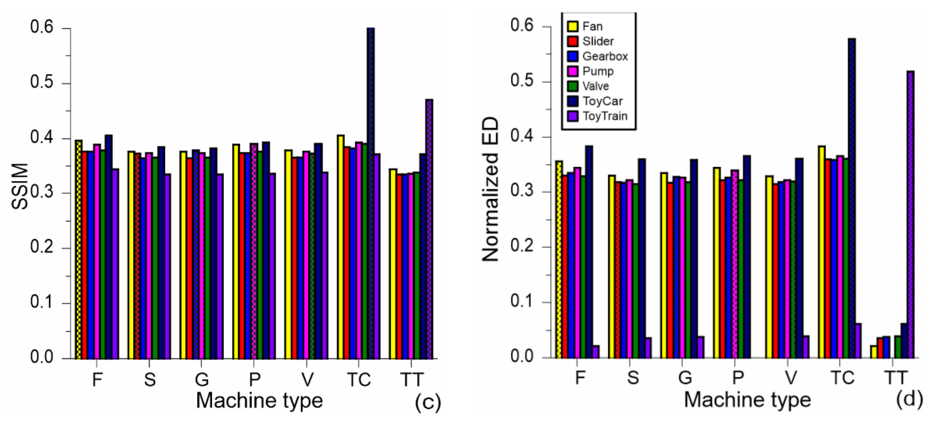
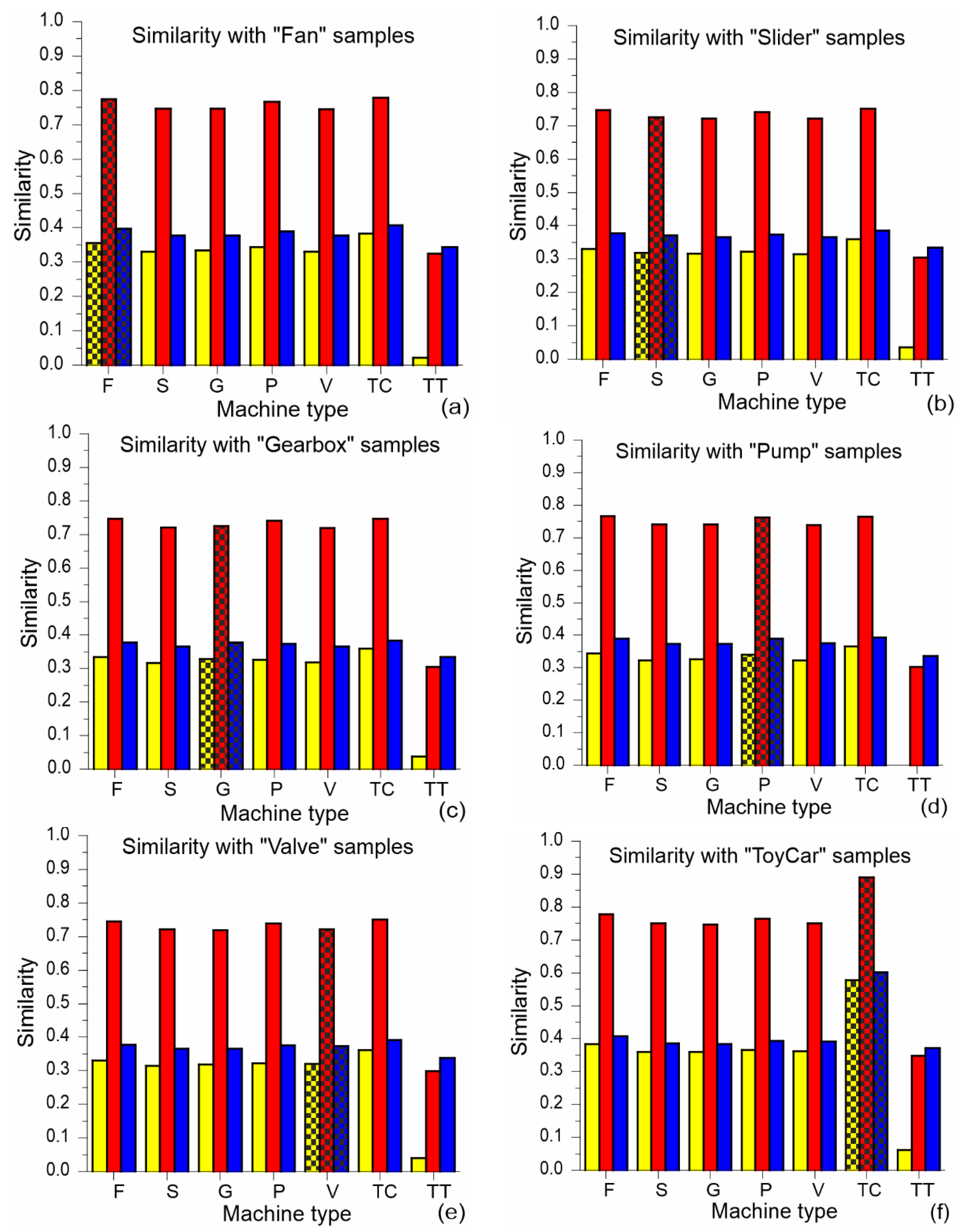
Visual comparisons of the mean intraclass and interclass similarity values are given in Figure 3 and Figure 4, wherein the intraclass similarity is presented by the hatched bars, while the interclass similarity is presented by the open (colored) bars. The order and color of the bars for the classes are the same in all the presented bar plots. Thus, the first bar in each set of bars for each particular class (machine type) represents the similarity for the fan class (yellow color), while the second one represents the slider class (red color), etc. The most obvious observation from these plots is that the greatest interclass similarity values are obtained for the pairing of toy-car with any other class (denoted as effect 1). It is interesting to note that these interclass similarities are even greater than the intraclass similarity for five classes—constituting all classes except toy-car and toy-train (effect 2). On the other hand, the smallest interclass similarity is obtained for the pairing of toy-train with any other class (effect 3). Comparing the noticed behavior in the results for the different similarity measures, all three effects are strong in the normalized ED. Effect 3 is prominent in all three similarity measures, while effects 1 and 2 are less prominent in the PCC and SSIM values.

Regarding the mutual relationships of the mean values of the employed image similarity measures from Figure 3, it can be seen that the ratios of the values for different classes are not the same in these measures. The smallest range of the mean values exists in the SSIM measure, where the differences between classes are smaller than in the normalized ED and PCC. In this way, the differences between classes are somehow blurred in the SSIM, which would suggest a slight advantage offered by the normalized ED and PCC compared to the SSIM in further analysis. The largest differences between two classes in the set of bars for any class from the group of five classes are present in the normalized ED. On the other hand, the values of the normalized ED depend on the particular value of ED_max used for ED normalization; hence, the PCC and SSIM are more objective measures.

The intraclass and interclass similarities for all three measures and given per machine type (class) are presented in Figure 4. The bar plots are rather similar for the group of five classes from fan to valve. Here, the interclass similarity of these classes with any other class except toy-train is close to the intraclass similarity (although the interclass similarity with toy-car is slightly higher than with other classes), while the interclass similarity with toy-train is the smallest. The bar plot for toy-car, presented in Figure 4f, shows that the intraclass similarity is greater than the interclass similarities, and this behavior is even more emphasized in the toy-train class (see Figure 4g).

Considering both the intraclass and interclass similarities, the classes from the group of five classes behave in a very similar manner. This phenomenon can be observed in Figure 2, Figure 3 and Figure 4. When the simplification of further analysis is beneficial, it would be appropriate to avoid considering all the classes from this group and instead choose only some of them, as performed here for certain analyses carried out using the fan and valve classes. The toy-car and toy-train classes have specific characteristics, making them very interesting for the next level of analysis.

4.2. Analysis at the Level of Image Similarity Measures Averaged Per Sample

The analysis at this level, which is more in-depth, is related to the mean of the similarity measures calculated for each individual sample (machine) in the similarity matrices, denoted here as the mean per sample. Specifically, the similarity values between a particular sample and all other samples from the same or different classes are located in a single row or column associated with that sample. The mean values per sample are calculated by taking the average of all values within a particular row or column. In this way, a vector with 3009 elements, that is, the mean values per sample, is generated separately for the intraclass and interclass similarity. Thus, we can see how each sample behaves, i.e., we can provide further insight, since the mean values provide only an overview of the general trends.

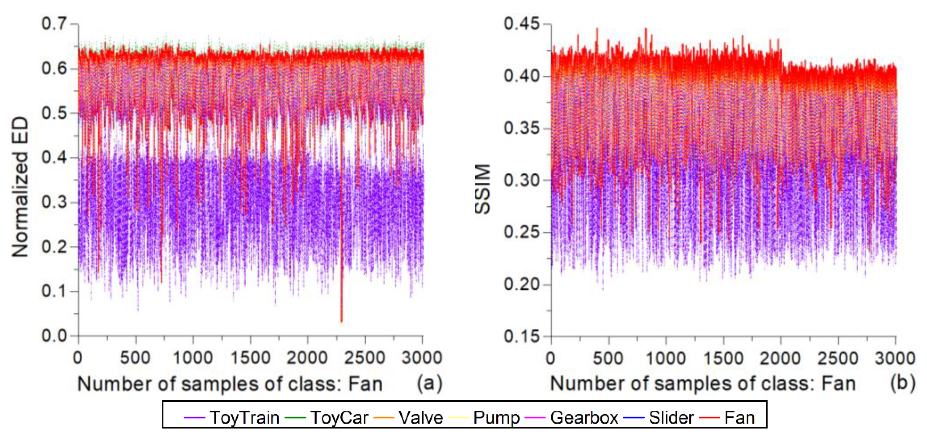
The line plots of the mean values per sample for two classes (toy-car and toy-train) and all three similarity measures are shown in Figure 5. The mean per-sample line for the intraclass similarity has greater values than the lines for the interclass similarities in all the presented cases. The normalized ED line plots for the toy-car class can be split into three groups ordered from the largest values to the smallest ones: the intraclass means, the interclass means for all pairings of the toy-car with any class from the group of five classes, and the interclass means between the toy-car and toy-train classes (see Figure 5a). The interclass normalized ED lines for the toy-train class have significantly smaller mean values per sample than those for the toy-car class, as shown in Figure 5b. Moreover, the means per sample for the toy-train class show a specific trend. Here, the samples of the toy-train class can be split into 12 sub-classes, wherein the separation between the sub-classes is represented by the stepwise shape of the intraclass and interclass line plots.

By comparing Figure 5a–d, that is, the results for the normalized ED and PCC, it can be seen that they are very similar, which implies that the main trends are the same. The minor differences observed are as follows: (a) the relative ratios of some intraclass and interclass lines are not completely the same, and (b) the spread of the values for the interclass lines in the results for the toy-train class is smaller in the normalized ED (Figure 5b) than in the PCC (Figure 5d).

The main trends seen in the results for the normalized ED and PCC are also found in the mean values of SSIM per sample. Thus, the largest mean values per sample for the toy-car and toy-train classes are found in the intraclass similarity (see Figure 5e,f). In addition, the toy-train class also has a very specific behavior here, manifested as an up-and-down stepwise shape of both intraclass and interclass lines associated with different sub-classes. The relative ratios of the similarity values of these sub-classes are not the same in different similarity measures.

In Figure 5, there is a certain overlap of the presented lines, especially those belonging to the group of five classes. Thus, the lines could hardly be observed individually; nevertheless, this is not the aim here. Instead, it is our intention to show the pattern and spread of the mean similarity values per sample at different levels, namely, (a) at the level of all the lines corresponding to either intraclass or interclass similarity, (b) at the level of all lines corresponding to a particular class, and (c) at the level of all lines corresponding to a particular similarity measure.

The overlapping of the line plots is even larger in the classes belonging to the group of five classes, which is shown as an illustration in Figure 6. The spread of the mean similarity values per sample in the individual lines for the fan samples is greater than the one for the toy-car and toy-train samples with respect to the results for all three similarity measures. This explains why the difference between the lines for different classes is not that obvious. The largest values belong to the interclass line for the toy-car class, which has slightly larger values than the intraclass line. The values of the intraclass line are similar to those of the interclass lines for all classes from the group of five classes. The smallest values belong to the interclass line for the toy-train class. Comparing the results for the normalized ED and SSIM, it can be seen that the main trends are the same, while there is a difference in the range of values for particular lines and their ratios.

4.3. Analysis at the Level of Image Similarity Measures for Individual Samples

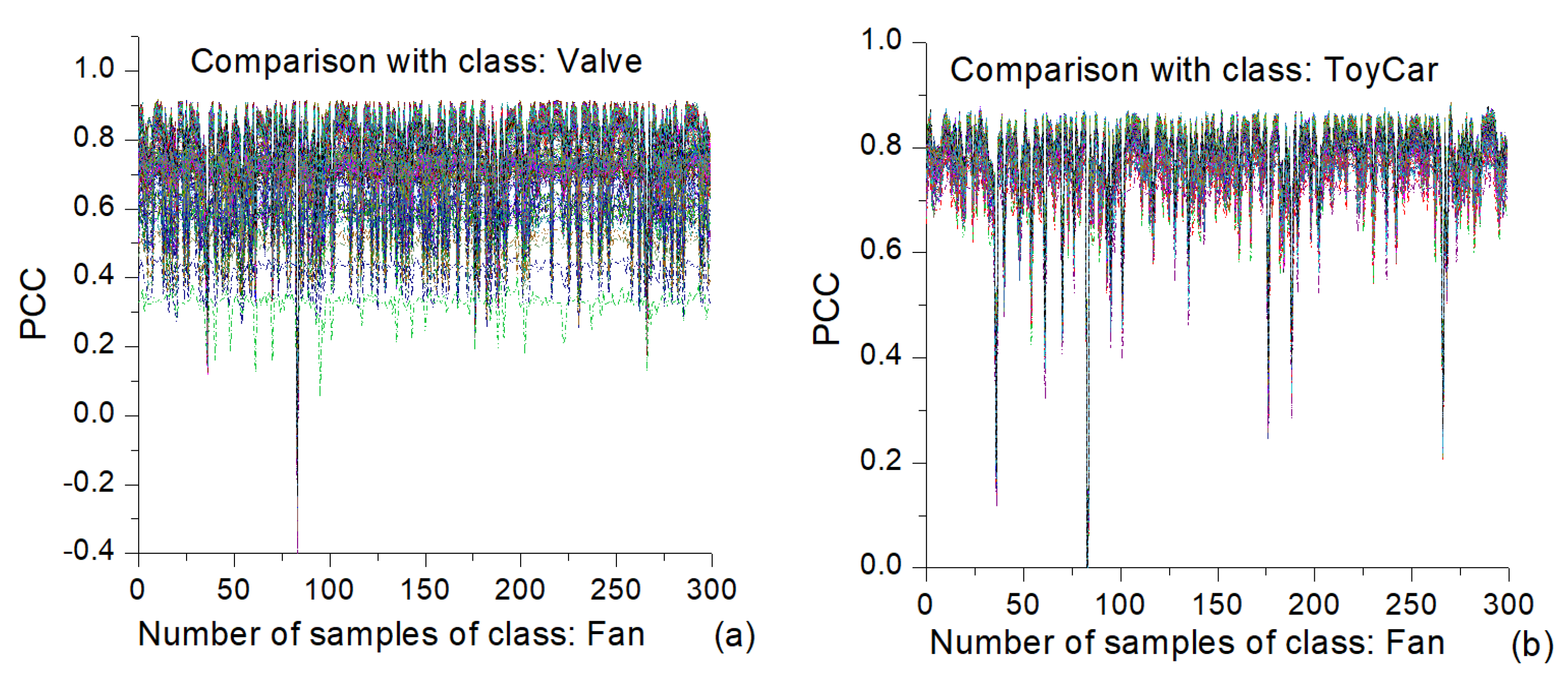
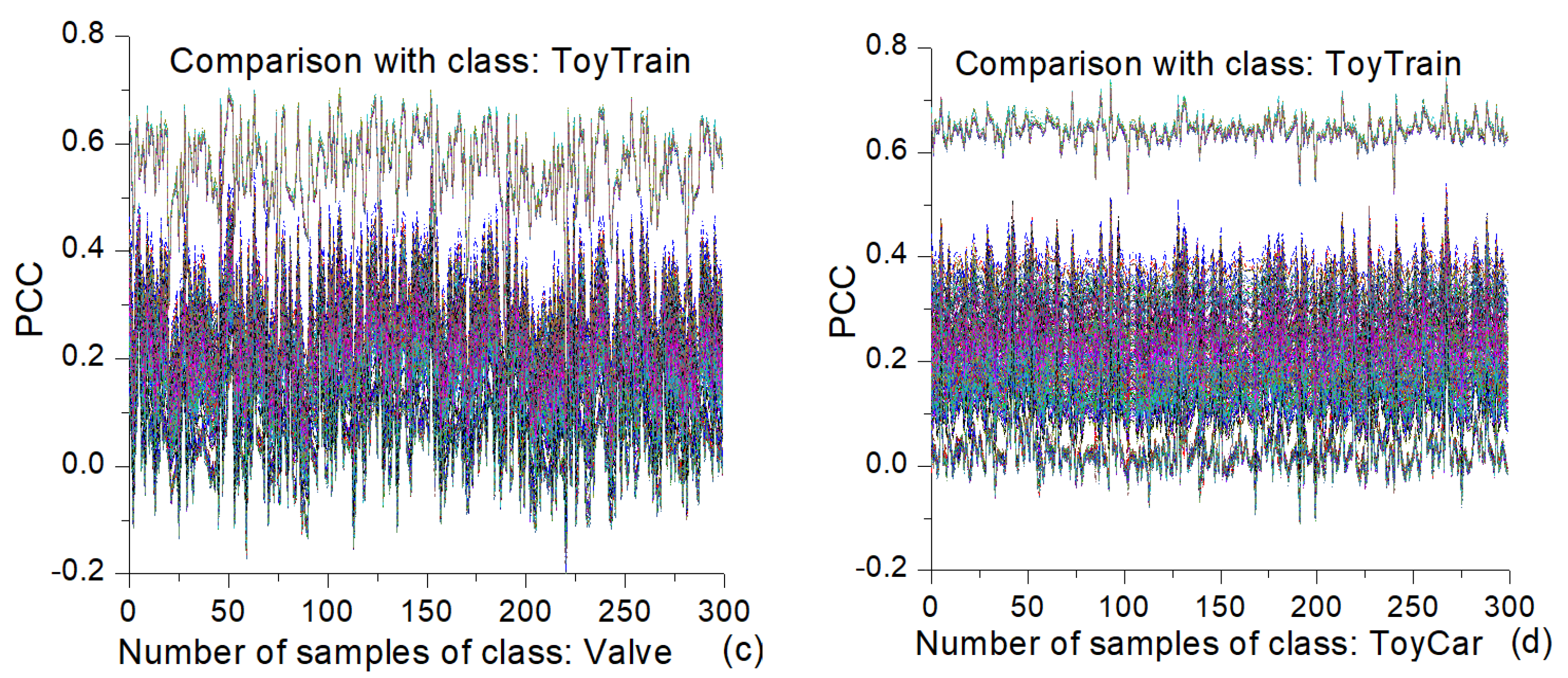
The image similarity measures for individual samples were analyzed using both the full and extracted datasets and via several analytical directions. The first direction is related to the visualization of the intraclass and interclass similarity matrices by means of heat maps. The second direction of analysis considers the similarity values in the form of line plots for every particular sample paired with all other samples belonging to the same class and different classes. Finally, the third analytical direction deals with the mel-spectrograms of the chosen samples with characteristic behaviors within a particular class or sub-class. The heat maps and line plots for all the similarity measures have been examined, but only those for the PCC are presented in this subsection. In order to visualize the details of these maps and plots, only the maps and plots generated from the extracted dataset are presented.

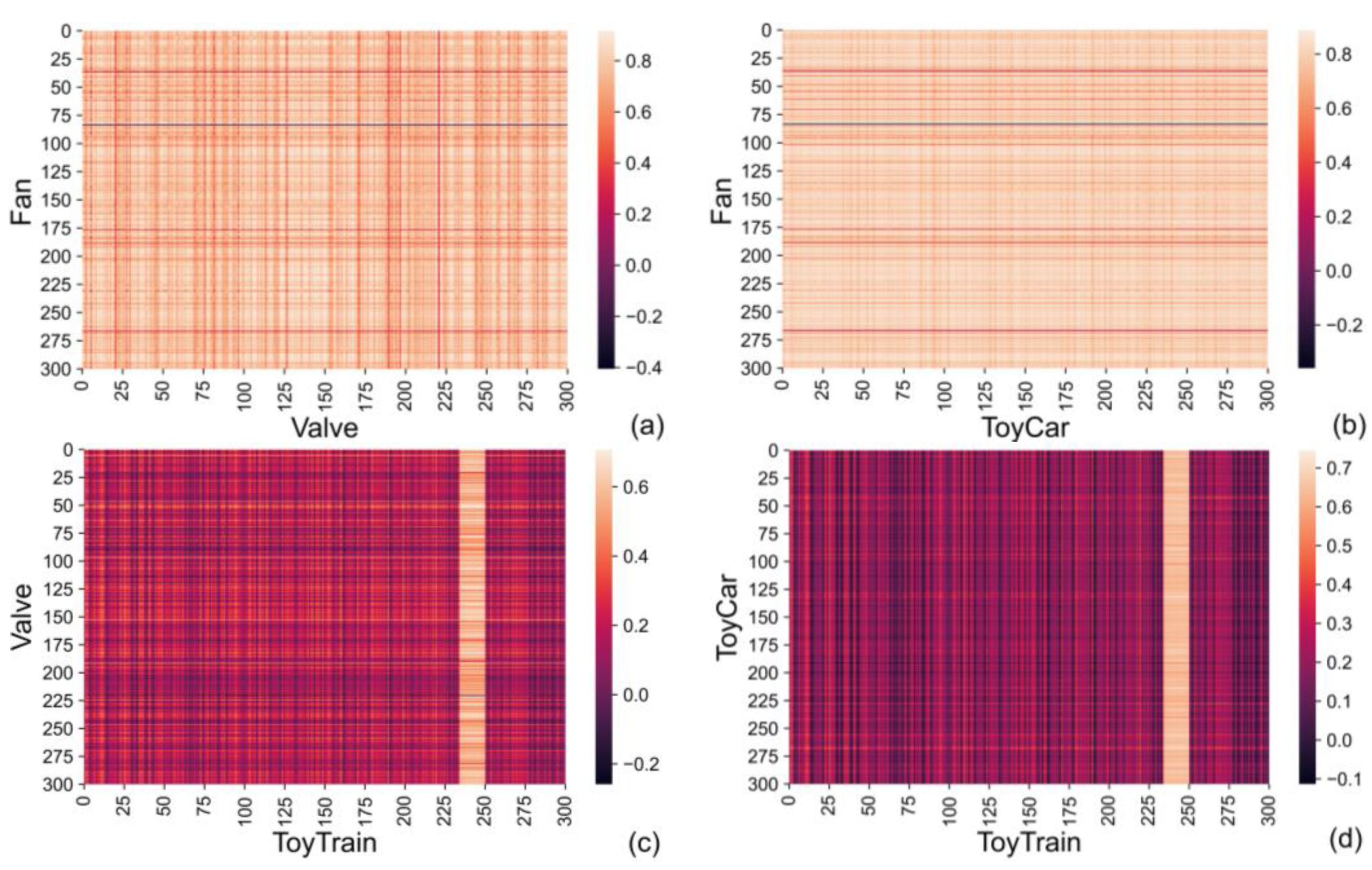
The intraclass similarity heat maps for four classes (fan, valve, toy-car, and toy-train) based on the PCC values obtained from the extracted dataset are shown in Figure 7. It is worth noting that the ranges of values in these maps are not the same, and the same color is associated with different values in different maps. Only few samples in Figure 7a have negative values with respect to the PCC, while all the PCC values in Figure 7b–d are positive. The majority of the fan samples have rather great PCC values (see Figure 7a). A similar situation exists with respect to the toy-car class, wherein the majority of samples have even greater PCC values, as shown Figure 7c. This is not the case with the valve samples, wherein there are samples with large to small PCC values (see Figure 7b). For these three machine types, it is interesting that the color is almost the same when moving along a particular line either in the horizontal or vertical direction. This means that a particular sample has similar PCC values with all other samples from that class present in the extracted dataset. On the other hand, the results for the toy-train samples are different: some samples can be grouped in sub-classes and further in sub-sub-classes (Figure 7d). This is manifested in the different colors of particular parts of the heat map, e.g., the dark-colored horizontal and vertical stripes or the light-colored squares in the bottom right of the heat map.

Similar patterns to those present in the intraclass PCC similarity heat maps from Figure 7 exist in the interclass PCC similarity heat maps. Four such heat maps are shown in Figure 8. The similarity values for a particular sample (machine) are rather consistent when moving along a horizontal or vertical direction representing the samples of one or another class, e.g., the fan and valve classes, as given in Figure 8a. The samples have different similarity values ranging from larger (closer to 1) to smaller (closer to 0), which are indicated by different colors shifting from lighter to darker, respectively. Samples with lower interclass similarity values are rare in the toy-car class in comparison to other classes; for example, observe the heat map values in the vertical direction in Figure 8b, where dark vertical stripes are hardly present. The most prominent characteristic of the toy-train class is the vertical, light-colored stripe found in both interclass similarities with the valve and toy-car classes (see Figure 8c,d). The different behavior of the toy-train samples within this stripe in comparison to the other toy-train samples is also visible in the intraclass similarity from Figure 7d.

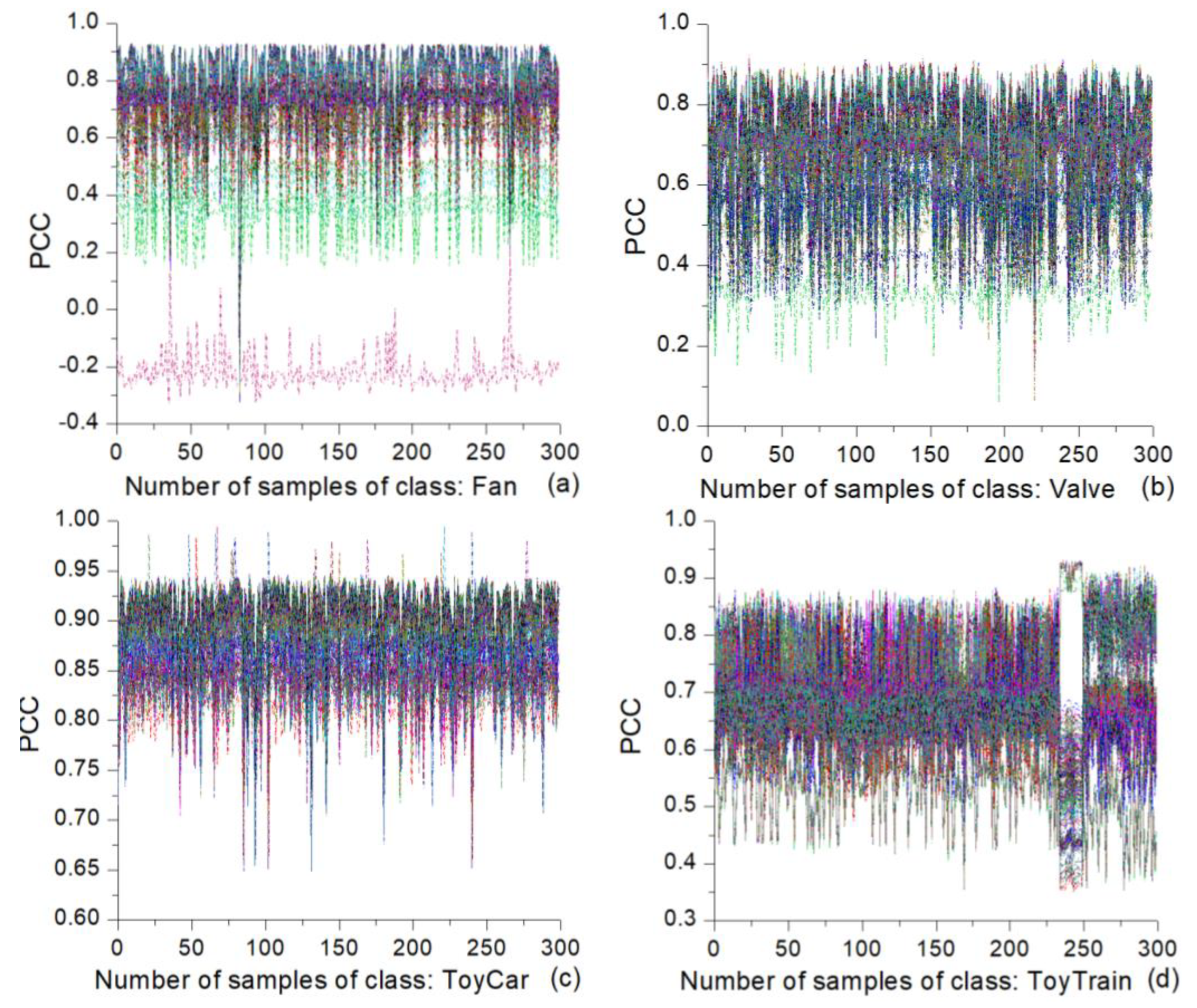
Figure 9 presents the intraclass PCC similarity line plots for four classes (fan, valve, toy-car, and toy-train). Each plot has 300 lines for the same number of samples present in each of those classes. In the fan samples (see Figure 9a), there is only one line in which the majority of its points have negative PCC values. This line belongs to a sample with a dark-colored line in the heatmap given in Figure 7a located in the vicinity of sample number 80. In all other lines, only very few points have negative PCC values, which are mainly associated with the above-mentioned sample. The samples from other classes in this figure do not have negative PCC values. The valve samples typically have values between 0.3 and 0.9, and the spread is rather large (see Figure 9b). On the other hand, the toy-car samples have the largest PCC values, and their spread is much smaller, as shown in Figure 9c, which is also observed in Figure 7c as the smallest variety of color of the heatmap. The majority of the values are between 0.80 and 0.95. As seen in the previous analysis presented herein, the toy-train samples show a different behavior. The majority of their PCC values range from 0.4 to 0.9 (see Figure 9d). There is a small sub-class of samples located in the vicinity of sample number 250 showing different characteristics.

The interclass PCC similarity line plots for the chosen pairs of classes are presented in Figure 10. Here, each plot also has 300 lines, wherein each line is associated with a particular sample of a class stated at the top of the plot. Each of these samples is paired with all the other samples from the other class stated below the x axis. Similar to the case of the intraclass similarity from Figure 9, the range of interclass similarity values for the fan–valve pair is between 0.3 and 0.9, as shown in Figure 10a. On the other hand, for the majority of the samples, this range is much smaller for the fan−toy-car pair (see Figure 10b). The interclass similarity values for the pairs valve−toy-train and toy-car−toy-train are smaller than those for the previously mentioned pairs (see Figure 10c,d).

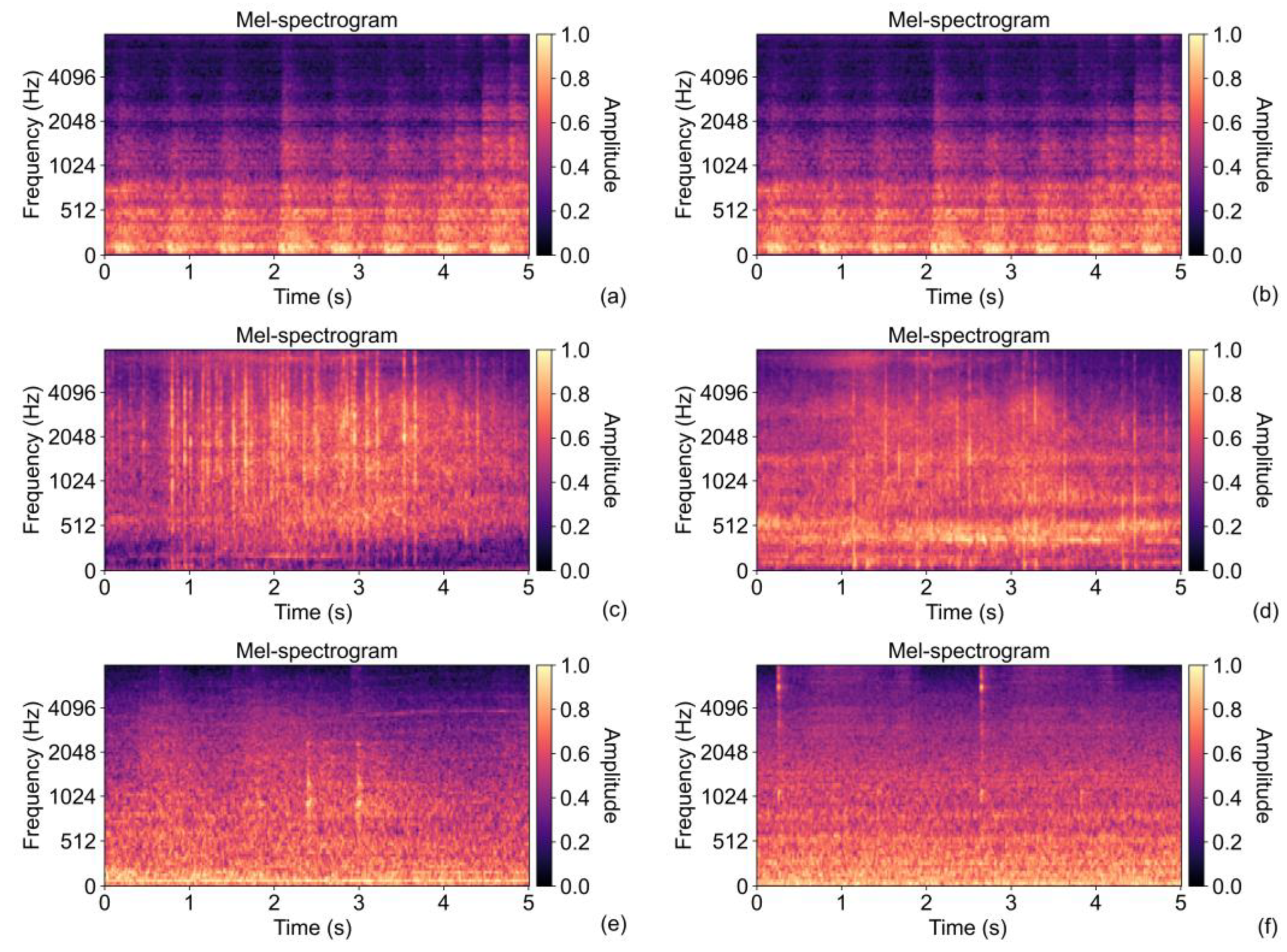
Some illustrative examples of the mel-spectrograms are shown in Figure 11, while their similarity values are summarized in

Table 4. Intraclass and interclass similarities of mel-spectrograms from Figure 11.

Machine-Type Pair	ED	PCC	SSIM
Toy-car no. 67—Toy-car no. 221	3.678	0.995	0.953
Toy-train no. 74—Toy-train no. 240	24.977	0.460	0.396
Toy-car no. 67—Toy-train no. 74	49.886	−0.012	0.248
Toy-car no. 67—Toy-train no. 240	38.597	0.586	0.355
Toy-car no. 67—Fan no. 150	27.832	0.779	0.359
Toy-car no. 67—Valve no. 238	29.672	0.815	0.395
Toy-car no. 221—Toy-train no. 74	49.141	−0.013	0.252
Toy-car no. 221—Toy-train no. 240	37.738	0.586	0.364
Toy-car no. 221—Fan no. 150	27.149	0.779	0.364
Toy-car no. 221—Valve no. 238	28.818	0.815	0.401
Toy-train no. 74—Fan no. 150	37.760	0.186	0.297
Toy-train no. 74—Valve no. 238	35.550	0.086	0.328
Toy-train no. 240—Fan no. 150	26.614	0.688	0.385
Toy-train no. 240—Valve no. 238	23.056	0.642	0.446
Fan no. 150—Valve no. 238	18.190	0.847	0.429

. Here, the mel-spectrograms given in Figure 11a,b, which are both from the toy-car class, are very similar to each other visually and according to the similarity values. On the other hand, the mel-spectrograms of two samples from the toy-train class (see Figure 11c,d) are not similar, or, more precisely, they are less similar than the toy-car samples. The mel-spectrograms of the fan and valve samples from Figure 11e,f, respectively, are similar to each other, and the degree of this similarity is moderate. Mutual similarities for different combinations of the samples can be found in Table 4.

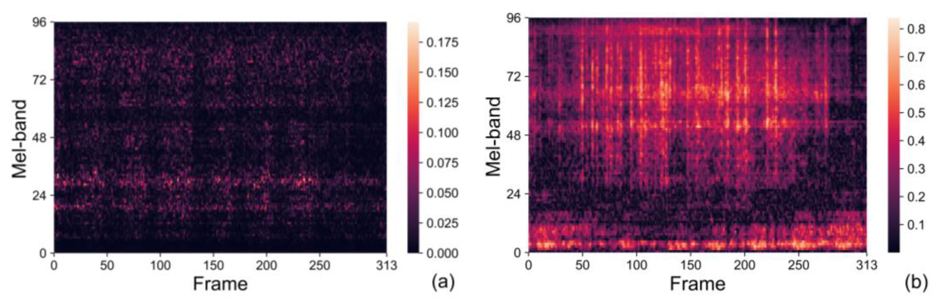
In order to demonstrate the possibility of linking the results of the image similarity estimation to the most distinctive features of the mel-spectrograms, the distance between two corresponding points was calculated for every single pixel of two compared images x and y, as given in Equation (3), but without summing the results. The illustrative examples in the form of a heat map are given in Figure 12, which compares two similar mel-spectrograms in Figure 12a (those from Figure 11a,b) and two dissimilar mel-spectrograms in Figure 12b (those from Figure 11a,c). The distance values between the similar mel-spectrograms are small, as indicated by the dark color in Figure 12a. The distribution of this dark color is rather uniform. Nevertheless, there are some vertical and horizontal stripes of a slightly brighter color that can be associated with particular components in either of the mel-spectrograms. On the other hand, the distance values in Figure 12b are greater than those in Figure 12a. Here, the bright color (large distance) is present at mid and high frequencies from approximately 1 s to 4 s, which is a consequence of the high levels present in the mel-spectrogram of toy-train number 74. The bright color is also present along the time axis at low frequencies, and it is caused by high levels in the mel-spectrogram of toy-car number 67.

5. Discussion and Comparison with Results from the Literature

Image similarity measures are compared from different perspectives in a number of references, e.g., [6,11,32,35]. Two-dimensional image similarity using SSIM, a modified feature-based similarity measure (MFSIM), a histogram-based SSIM (HSSIM), and one-dimensional similarity using cosine similarity, Pearson correlation, Tanimoto similarity, and angular similarity are tested in [5]. The related results showed that HSSIM and MFSIM in 2D similarity analysis as well as cosine similarity and Pearson correlation in 1D similarity outperform other measures. In another study [6], the accuracy of five similarity measures—correlation coefficient, ED, S1-score (S1), SSIM, and average hash (aHash)—is compared with respect to extracting sea level pressure patterns. The highest accuracy was obtained by applying S1 and SSIM, and these two measures can give results closer to the subjective similarity between two maps than ED.

In [6], the accuracy of three conventional similarity measures—correlation coefficient, ED, and S1 score—is evaluated with respect to the analog method. Two measures or norms often used in practice—L1 (Manhattan distance or sum of absolute error) and L2 (ED or sum of square error), representing specific instances of the Minkowski metric—are compared in [9], wherein a small and consistent preference is given to the L1 measure. This measure may capture human notions of image similarity in a better way. In [32], the normalized MI for maximizing the similarity during inter-frame registration and the 2D correlation coefficient for absolute alignment and quality control are suggested as preferable measures. In another study, the performance of the SSIM is shown to be superior to that of PSNR in image quality assessment [4]. On the other hand, the calculation of the SSIM is more demanding and time-consuming than the calculation of the PCC. An example is given in [4], where the calculation of the SSIM was about 125 times longer than the calculation of the PCC.

In [6], it is stated that the identification of a single similarity measure that shows good performance when applied to diverse problems is a very difficult task. It is also difficult to determine a measure that can completely capture visual resemblance [6]. Apart from other factors, the performance of an image similarity measure also depends on the application and its properties, as well as the method used to measure the degree of matching [32].

Although there are a dozen image similarity measures, it seems that there is a high degree of correlation between them [36], and it is not necessary to use all of them. This means that many of those measures calculate the “same property” between two images, essentially, variance [39]. In other words, all these measures represent only a small number of independent degrees of freedom. Despite the high correlation among the measures, it has also been concluded that it is not enough to consider only one measure [36].

A number of analyses of image similarity measures from the literature are related to subjective similarity or visual resemblance, that is, the human notion of image similarity. In the present research, this aspect of image similarity is not of primary importance. The images whose similarity is analyzed herein are not natural images. Instead, they are generated in a specific way by applying a transformation or mapping of an industrial product’s (machine) sound into a particular image, that is, the mel-spectrogram, in this case. So, preference is given to a measure or measures that can clearly distinguish between the types of industrial products (classes) based on certain properties of the images obtained from the products’ sound.

It is not an easy task to specify which target image properties should be used for the mentioned purpose. The applied industrial product sounds consist of the sounds of particular products, but also some other disturbance sounds coming from the environment, e.g., sounds produced by other machines. These two sounds—the target product’s sound and disturbance sound—are mixed together and their contributions (counterparts) are also mixed together and distributed throughout the generated image. It is typically rather difficult to discriminate the specific parts of the mel-spectrogram belonging to either of these two sounds.

Another important issue is the position of a characteristic part (detail) in the image, for example, the position of a particular harmonic. The two axes of a mel-spectrogram image belong to different domains, where the x axis is the time-domain axis and the y axis is the frequency domain axis. A translation or shift along the x axis means that a certain sound object exists at different time while a shift along the y axis means that the characteristic of that sound object has changed. Thus, it can be considered that this is no longer the same sound object.

From the viewpoint of classification or detection tasks, it would be beneficial to have a level of intraclass similarity as large as possible and a level of interclass similarity as small as possible with respect to the analyzed mel-spectrograms. From this perspective, the three image similarity measures used here (ED, PCC, and SSIM) behave in a similar way. A mean intraclass similarity larger than any other mean interclass similarity is clearly seen in only two classes, namely, the toy-car and toy-train. The mean intraclass similarity of any class from the group of five classes (fan, slider, gearbox, pump, and valve) is rather similar to the mean interclass similarities between these classes. Here, this does not mean that there are no samples (machines) whose similarity with other machines from the same class (product type) is not considerably greater than the one with machines from other classes. However, there are also samples that are more like the samples from other classes than the samples from the same class. Moreover, the spread of the image similarity values for a particular sample when compared to other samples from the same and different classes is large, and the number of such samples in some classes is also large. This is especially true for the SSIM measure.

Various criteria can be used to mutually compare the image similarity measures in the case of mel-spectrograms; the ones applied here include: (a) the maximum possible intraclass similarity, (b) minimum possible interclass similarity, (c) the maximum possible separation for a range of interclass similarity values when different classes are mutually compared, and (d) the minimum possible spread of similarity values for an individual sample (machine) when compared with samples from a particular class. According to the mentioned criteria, the SSIM measure has the worst ranking, while the other two measures (ED—that is, the normalized ED—and PCC) are rather similar to each other. The SSIM’s rank might be a consequence of the inherent characteristics of this measure with respect to recognizing certain “structures” of an image independently on their position within the image. Moreover, it is known that the performance of the SSIM is worse in images with noise, blurred images, and images very similar to each other. On the other hand, the results for the normalized ED and PCC are similar at both levels, namely, the level of statistical quantities and that of individual samples. A weak point of these two measures is that equal weighting is given to all image points (pixels), or, more precisely, no weighting is applied.

Another relevant aspect when comparing the three similarity measures is their computational efficiency. Here, this aspect is considered by means of the computation time (response time) needed to calculate the intraclass similarity for all seven classes and the full dataset (3009 samples). The approximate number of image comparisons to perform such a calculation for a single measure is 63 million. The computation time was measured while the Python code is executed on a computer with an Intel Core i7-8700 3.2 GHz 6-Core LGA 1151 processor with six cores operating at 3.2 GHz, 32 GB of RAM, and running the Windows 10 Education operating system. As previously described, the calculation of the ED and PCC measures first requires one to make arrays from the mel-spectrogram images, which takes 21.76 s. The calculation itself lasts 65.96 s for ED and 228.20 s for the PCC, which finally yields computation times of 87.72 s and 249.96 s for ED and the PCC, respectively. On the other hand, the SSIM is calculated directly from the mel-spectrograms, and the time needed for this calculation is 1013.79 s. Therefore, in circumstances wherein algorithm complexity or computation time plays an important role in choosing which measure to use, the use of ED is more advantageous than the PCC and SSIM.

The similarity estimation for images obtained from sound can be improved by including weights to certain objects of the image that are closely related to the sound of a target product. Another method for improving the estimation of sound-related image similarity is the use of a weighted combination of the three analyzed similarity measures

$$Q=w_1\cdot E{D}_{normalized}+w_2\cdot PCC+w_3\cdot SSIM,$$

(9)

where Q is a new image similarity measure, while w₁, w₂, and w₃ are the weights of the ED, PCC, and SSIM, respectively, whose sum is equal to 1. Complementary information present in any of the three similarity measures will be translated to the new similarity measure. The obtained results suggest that somewhat greater weights should be given to the ED and PCC as opposed to the SSIM.

The approach based on image similarity estimation can be employed for solving important industrial problems, such as fault diagnostics, that utilize machines’ sound. Here, the hypothesis is that the sound of a faulty machine is sufficiently different from a non-faulty one, that is, their mel-spectrograms are sufficiently different from each other. If this is not the case, either another image representation (e.g., a full-resolution spectrogram) or a detection algorithm should be applied. Since the performance of the ED in the mel-spectrogram similarity estimation is not worse than that of the other two measures, and as this measure is more computationally efficient, the ED constitutes a preferable option for implementation in embedded and real-time systems.

6. Conclusions

Herein, the similarity of images generated by mapping the sounds of seven types of industrial products (machines) into mel-spectrograms is analyzed by applying three image similarity measures often used in the literature: ED, the PCC, and SSIM. Mel-spectrograms represent an image commonly applied as an input to diverse, audio-based DNN algorithms, especially CNN algorithms. Two datasets were included in this research, namely, the full dataset and the extracted dataset containing 3009 and 300 sound samples, respectively, in each machine type (class).

By investigating the obtained results at different levels of generality, it has been concluded that, according to their image similarity values, the seven classes of machines can be split into three groups: a group of five classes (fan, slider, gearbox, pump, and valve) and toy-car and toy-train groups. In the first group, at a general level of analyzing the statistical quantities, the intraclass similarity is either only slightly greater or even smaller than the interclass similarity. Moreover, the difference among the interclass similarities when different classes from this group are compared to each other is rather small. This is not the case for the toy-car and toy-train classes, thus showing a clear distinction between the intraclass and interclass similarity and among interclass similarities when comparing different classes. At the level of the results for the individual samples, image similarity values for a particular sample when compared to other samples either from the same class or different classes can show significant deviations from the main trend for this class. In some situations, it is even very difficult to find the main trend. On the other hand, there are some very consistent results with a narrow spread of similarity values for the majority of samples of a particular class. Such behavior is seen mainly in the toy-car and toy-train classes.

Regarding the comparison of the applied image similarity measures, the more consistent results and clearer distinctions between classes are found when using the ED and PCC compared to the use of the SSIM measure. There is a significant correlation among these measures which provided redundant information, as the same main trends are seen in the results for all three measures. However, it seems that using only a single image similarity measure in the present form would not provide enough information in order to develop a fully functional parametric classifier based on image similarity values. In order to develop such a classifier that can provide comparable results to those based on DNNs, it would be necessary to obtain more reliable and consistent information from image similarity estimation.

Future work can be related to the modification of the existing image similarity measures so as to render them more relevant for images generated from sound, such as spectrogram-like images. The existing image similarity measures or these modified versions can be applied to other images generated from sound such as gammatonegrams or auditory image maps.