Article

The Evolutionary Dynamics of a Sex-Structured Population with Non-Overlapping Generations

1
Institute for Complex Analysis of Regional Problems, Far East Branch, Russian Academy of Sciences, 679016 Birobidzhan, Russia
2
Institute of Automation and Control Processes, Far Eastern Branch, Russian Academy of Sciences, 690041 Vladivostok, Russia
*
Author to whom correspondence should be addressed.
Mathematics 2023, 11(24), 4971; https://doi.org/10.3390/math11244971
Submission received: 25 October 2023 / Revised: 2 December 2023 / Accepted: 13 December 2023 / Published: 15 December 2023
(This article belongs to the Special Issue Mathematical Modeling of Evolutionary Dynamics)

Abstract

:
This paper proposes and studies a discrete-time model for a sex-structured population with non-overlapping generations under density-dependent regulation of survival. The population is assumed to have genetic variety among individuals in terms of reproductive potential, controlled by a single autosomal diallelic locus. We consider a panmictic population with Mendelian inheritance rules. We examine the stability model and show that increasing the average value of reproductive potential destabilizes the population dynamics. The scenario of stability loss in fixed points via period doubling or Neimark–Sacker bifurcations depends on the intensity of the self-regulation. The growth rate at which the population survives and develops is shown to depend on the fitness of the genotypes and the secondary sex ratio. As a result, the asymptotic genetic composition of the population is determined by the values of the reproductive potentials of the heterozygote and homozygotes, the initial conditions, and the parameter describing the ratio of newborn females to males. With disruptive selection, the influence of external factors changing the current genetic composition of a population can alter the direction of evolution and lead to the extinction of a successful developing population or a gradual population recovery due to evolutionary rescue after a noticeable decline in its abundance.

1. Introduction

The fundamental principles of general biology that pertain to population evolution and ecosystem dynamics were established under the assumption that ecological and evolutionary processes are interconnected and that their interactions can be significant. In particular, the author of the theory of evolution, Charles Darwin (Darwin, 1859), the creators of the synthetic “genetic” theory of evolution, R. Fisher (1930), S. Wright (1930), J. Haldane (1932), and S.S. Chetverikov (1926), as well as the founders of theoretical ecology, P. Verhulst (1847) and V. Volterra (1928) (as well as G.F. Gause (1935)) [1,2,3,4,5,6,7,8], considered evolutionary and ecological processes as integral characteristics of a whole. Additionally, the study of ecological and evolutionary dynamics assumes that organisms’ life cycle features can evolve on a similar timescale as their population dynamics [9,10,11]. On the one hand, changes in genetic structure occurring during the evolution of a population (primarily under the influence of natural selection) affect the birth rate and, accordingly, its dynamics. On the other hand, as a rule, fluctuations in abundance are caused by changes in the population structure caused by the combined effects of environmental factors and self-regulatory mechanisms [12,13,14]. Therefore, when modeling population dynamics, it is advisable to use an ecological–genetic approach that allows us to study the interconnected changes in the abundance and genetic structure of a population [15,16,17,18,19,20,21,22,23,24,25,26,27].
Within the approach combining classic population genetic theory and ecological modeling, the dynamics of genetic frequencies are studied depending on various inheritance patterns and using the relative fitness values of genotypes, which allows for considering the population abundance to be constant without analyzing its dynamics [2,28]. This approach remains relevant today (e.g., [29,30,31]). A modification of unstructured ecological models by including genotype fitness as a function of intra- and interspecies density [16] further develops this approach. In parallel, population genetics extends by considering both age [32,33,34] and sex [35] structures. The concepts of density- and frequency-dependent components in the action of natural selection have been developed [32,33,34], as have density-independent forms of natural selection, whose action under ecological limitation can cause a change in the nature of the population abundance dynamics [36,37,38]. Currently, research continues to investigate the relationship between population genetics, stage (age) [23,24,25,26,39], and sex [22] structures. The work [22] derives conditions for protected polymorphism in a population characterized by age- or stage-dependent demography with two sexes.
Additionally, within the synthetic theory, there are studies using simplified models of evolution that do not consider genetic dynamics in detail, i.e., they do not imply a detailed description of the inheritance mechanism of the traits under consideration. In such studies, as a rule, the evolution of polygenic and continuously distributed traits (or quantitative traits [40]) is modeled (e.g., [41,42,43,44,45,46]), as is the evolution of clonal systems in which individuals have separate discrete trait values and ideal inheritance of phenotypes, disturbed by rare mutations [41,44,46,47,48]. In general, despite the large number of papers and diversity of studied objects, unresolved issues remain related to the dynamics and evolutionary features of structured populations and the study of their regulatory mechanisms.
On the other hand, combining classic population genetic theory and ecological modeling makes it possible to see the effects that are missed when using each of these approaches in isolation, as well as to study the interconnected changes in the abundance and genetic structure of a population under ecological limitation during the influence of natural selection [20,21,22,23,24,25,26,27,49,50,51,52]. Examples include the effects of bottlenecks, evolutionary rescue, or degeneration, in which genotype ratios determine the growth or decline of population abundance. Note that sometimes there is a catastrophic decrease in population size up to several reproductive pairs (individuals), which are subject to the threat of extinction. A small population that is in danger of extinction still has two possible development options: to become extinct or to adapt with a subsequent recovery of the population size after passing through a “bottleneck” [53]. Note that massive non-selective mortality allows only a few individuals to pass on their genes to subsequent generations. Consequently, a temporary reduction in population size (bottlenecks in population size) can affect the genetic variability, mutation load, and inbreeding levels in populations [53,54,55,56]. When endangered species manage to adapt to changes in the environment within sufficiently short time frames to prevent their extinction, this is referred to as evolutionary rescue [56,57,58]. Examples of natural populations that have temporarily passed through a bottleneck include the following: Mexican and red wolfs [59], island gray Californian foxes [60], Mednyi arctic fox [55], northern elephant seal [61], European bison [62], and cheetah [63]. The natural interconnection of ecological and genetic processes and the discovered effects that are observed in biological populations confirm the promise and importance of developing eco-evolutionary approaches. Maintaining genetic polymorphism is a crucial issue in population genetics [22,23,24,28,52,64,65,66,67,68,69], since a reduction in genetic variety combined with genetic drift and inbreeding can lead to unpredictable and even catastrophic consequences for the population. Thus, among the main results of population genetics are the criteria that determine whether natural selection leads to the fixation of one genotype or the coexistence of several genotypes with polymorphism [28,30,47,65,66,67,68,70]. For example, the lack of genetic variety in cheetahs led to abnormalities in sperm formation, reduced fertility, high infant mortality, and increased susceptibility to diseases [71].
The present work is devoted to the development of an eco-genetic approach to modeling the dynamics of limited sex-structured populations with non-overlapping generations within mathematical biology. We propose a dynamic model of a population that is structured by sex, which allows for studying evolutionary processes. Note that adding sex structure to the model is important for understanding population abundance fluctuations, since sexual reproduction is one of the essential mechanisms of microevolutionary transformations and animal adaptation to the environment. The model assumes that density-dependent factors limit the survival of females and males at different intensities. In addition, we consider a population with genetic diversity in individuals’ reproductive potentials, controlled by one autosomal diallelic locus. Note that mathematical models rarely incorporate population genetic equations without simplifying Mendelian inheritance principles. The unpopularity of single-locus models is related to the ingrained notion of polygenic control of phenotypic traits. Increasing the number of loci that are considered significantly complicates the models and quickly deprives them of the possibility of adequately interpreting simulation results. However, using a single-locus diallelic inheritance model is quite justified; in particular, one of the principal lifecycle traits of the arctic fox is litter size, which is genetically determined by a single diallelic locus [72].
This paper aims to study the evolutionary dynamics of an ecologically limited population that is structured by sex with seasonal reproduction and non-overlapping generations. The reason for choosing populations with non-overlapping generations and a short life cycle with a limited breeding period is the occurrence of significant fluctuations in the abundance of such species [73,74,75,76,77,78]. An example of such a species is the larch bud moth, for which genetic polymorphism is one of the main factors regulating its abundance [79,80]. At an excessively high density, the genetic structure of the insect population changes, accompanied by the emergence of morphological forms that differ in several traits. In particular, dark-colored ecotypes are more sensitive to food quality, and their predominance during defoliation accelerates the completion of the population abundance peak phase [79]. Additionally, this species is affected by ecological limitations due to decreasing food availability.
The present study continues a series of papers that is devoted to the dynamics of a limited population with sex structure [81,82,83,84], focusing on ecological modeling. This study considers changes in the reproductive potential of a population during evolution under the influence of natural selection. Consequently, the proposed model combines an ecological model of the dynamics of a limited population with non-overlapping generations represented by females and males with a microevolutionary model of the dynamics of the population’s genetic structure. We analyze the bistability of monomorphic solutions. We deliberately make minimal assumptions about the ecological structure of the population. A relatively simple model allows us to consider the influence of genotype reproductive potentials, secondary sex ratio (proportion of newborn females), and intraspecific competition on the dynamics of a sex-structured population and its genetic composition.

2. Model Assumptions

Let us consider a population with seasonal breeding, consisting of females and males. The parental generation dies before the new breeding season starts, ensuring non-overlapping population generations. Some species of plants, insects, fish, zooplankton, and birds have non-overlapping generations.
We consider the time step in modeling n to be the interval between breeding seasons. We assume that the number of females determines that of newborns, and the survival rates of females and males differ due to intraspecific competition and depend on population abundance.
In addition, we assume that there is genetically determined variety among individuals in the population, differing in reproductive potential (the maximum of their possible fecundity). To understand the basic outcomes of natural selection in a considered population, we can study a simple case where a single diallelic locus with alleles A and a encodes fitness. We assume that genes located on non-sex chromosomes (autosomes) control the reproductive potential, and there are three genotypic groups, AA, Aa, and aa, in the population, with different reproductive potentials that are equal to rAA, rAa, and raa, respectively. Since the gene is autosomal, these three genotypic groups exist in both sexes for this trait.
Let us assume that the population is panmictic, i.e., that there is free mating between individuals with different genotypes, and Hardy–Weinberg equilibrium holds, linking genotype frequencies and allele frequencies [35]. In this case, to describe the dynamics of the population’s genetic structure, it is sufficient to consider the frequency dynamics of one of the alleles; for certainty, it will be the dynamics of allele A. It is easy to show that for a population with non-overlapping generations, after the first panmictic mating, the allele A frequencies in females and males of the offspring equalize, and their further dynamics do not differ (Appendix A).
As mentioned earlier, the ecological limitation of population growth is assumed by a decreasing female and male survival with an increasing total abundance [18]. We consider the linear decrease with different limitation (or competition) coefficients for females and males. Moreover, the limitation is suggested to not depend on the genotype, i.e., the survival of all female genotypic groups decreases with an increasing abundance according to the same law, and the same is true for the male genetic groups. The difference in male and female limitation coefficients does not lead to a difference in gene frequency dynamics in either sex of the populations. Then, one equation can describe the dynamics of allele A frequency in the population.

3. Model Description

The above assumptions are sufficient to obtain the following system of recurrent equations to describe the dynamics of female and male abundances, as well as allele A frequency in a population with non-overlapping generations and a genetic variety in individuals in terms of reproductive potential (Appendix A):
F ( n + 1 ) = δ r ¯ ( n )   F ( n ) ( 1 β 1 ( F ( n ) + M ( n ) ) ) M ( n + 1 ) = ( 1 δ ) r ¯ ( n ) F ( n ) ( 1 β 2 ( F ( n ) + M ( n ) ) ) p A ( n + 1 ) = p A ( n ) ( r A A p A ( n ) + r A a ( 1 p A ( n ) ) / r ¯ ( n ) ,
where n is the breeding period number; F (F ≥ 0) and M (M ≥ 0) are female and male abundances, respectively; p A ( n ) ( 0 p A 1 ) is the frequency of allele A in the n-th generation; β 1 ( β 1 0 ) and β 2 ( β 2 0 ) are limitation coefficients describing the intensity of intrapopulation competition; and δ ( 0 δ 1 ) is the proportion of newborn females. Parameters r A A , r A a , and r a a ( r A A , r A a , r a a 0 ) are the reproductive potentials of genotypes AA, Aa, and aa, respectively; r ¯ ( n ) = r A A ( p A ( n ) ) 2 + 2 r A a p A ( n ) ( 1 p A ( n ) ) + r a a ( 1 p A ( n ) ) 2 , r ¯ > 0 is the average reproductive potential of individuals in the population in the n-th breeding season.
After the transition to relative abundances ( F β 2 f , M β 2 m ), we obtain equations for the evolutionary dynamics of a population with two sexes in a simplified form:
f ( n + 1 ) = δ r ¯ ( n )   f ( n ) ( 1 ρ ( f ( n ) + m ( n ) ) ) m ( n + 1 ) = ( 1 δ ) r ¯ ( n ) f ( n ) ( 1 ( f ( n ) + m ( n ) ) ) p A ( n + 1 ) = p A ( n ) ( r A A p A ( n ) + r A a ( 1 p A ( n ) ) / r ¯ ( n ) ,
where ρ = β 1 / β 2 ( ρ 0 ) denotes a parameter that characterizes the relative contribution of mature individuals to the limitation of the population survival process.
The first two equations of system (2) describe the dynamics of female and male abundance when the average reproductive potential r ¯ ( n ) changes during microevolution. The third equation of system (2) corresponds to the dynamics of the A gene frequency, which determines reproductive potential, i.e., the microevolution process itself.

4. Fixed Points and Their Stability

In the third equation of system (2), the change in allele A frequency under the influence of natural selection does not depend on the first two equations. This means that the frequency of allele A (value pA) in the model under consideration does not depend on the numbers of females and males. The change in the frequency of allele A, i.e., for one generation, equals
Δ p A = p A ( n + 1 ) p A ( n ) = p A ( n ) ( r A A p A ( n ) + r A a ( 1 p A ( n ) ) r A A ( p A ( n ) ) 2 + 2 r A a p A ( n ) ( 1 p A ( n ) ) + r a a ( 1 p A ( n ) ) 2 p A ( n ) .
We find the equilibrium values of the frequency of allele A by equating Δ p A = 0 , i.e., p A ( 1 p A ) p A ( r A A 2 r A a + r a a ) + r A a r a a ( r A A 2 r A a + r a a ) p A 2 ( n ) + 2 ( r A a r a a ) p A + r a a = 0 .
It follows from the last equation that in system (2), three equilibrium genetic structures are possible, in which the equilibrium frequency of allele A takes the values of either p ¯ A = 0 , or p ¯ A = 1 , or p ¯ A = p * , where p * = ( r a a r A a ) / ( r A A 2 r A a + r a a ) , 0 < p * < 1 , which is the same as in the evolution model of a homogeneous population [38,66,85]. The first two equilibrium states are monomorphic and correspond to the complete displacement of one allele by another. The third equilibrium corresponds to the maintaining polymorphism in the population, i.e., the population has both alleles A and a, and in general, all three genotypes are present: AA, Aa, and aa.
Substituting stationary values r ¯ into the first two equations of system (2) gives the values of female and male population numbers. Let us present all the stationary states of system (2).
System (2) has three fixed points with zero numbers of females and males, of which two are monomorphic— E 0 ( 0 ,   0 ,   0 ) (by allele a) and E 1 ( 0 ,   0 ,   1 ) (by allele A), and one is polymorphic— E 2 ( 0 ,   0 ,   p * ) . Fixed points E 0 , E 1 , and E 2 correspond to population extinction.
In addition, model (2) has three fixed points with a non-zero population size:
  • Monomorphic fixed point E 3 ( f ¯ ,   m ¯ ,   0 ) with respect to allele a has the following coordinates:
    f ¯ = ( 1 r a a δ ) / r a a ( ρ 1 ) δ ( r a a ( δ 1 ) 1 ) 1 , m ¯ = ( 1 δ ) ( 1 + r a a ( ρ 1 ) δ ) / ( δ ρ   f ¯ ) ,   p ¯ A = 0 ,
    where r a a > 1 / δ .
    In this case, females and males in the population are represented only by individuals with the aa genotype, while the AA and Aa genotypes are absent.
  • Monomorphic fixed point E 4 ( f ¯ ,   m ¯ ,   1 ) with respect to allele A has the coordinates
    f ¯ = ( 1 r A A δ ) / r A A ( ρ 1 ) δ ( r A A ( δ 1 ) 1 ) 1 ,   m ¯ = ( 1 δ ) ( 1 + r A A ( ρ 1 ) δ ) / ( δ ρ   f ¯ ) ,   p ¯ A = 1 ,
    where r A A > 1 / δ . The fixed point E 4 ( f ¯ ,   m ¯ ,   1 ) corresponds to the situation when the population consists of individuals from both sex groups with only the AA genotype.
  • Polymorphic fixed point E 5 ( f ¯ ,   m ¯ ,   p * ) has the coordinates
    f ¯ = C ( B δ C ) / ( ( ( ρ 1 ) B δ 2 ( B + C ) ( ρ 1 ) δ C ) B ) , m ¯ = ( 1 δ ) ( ( ρ 1 ) B δ + C ) C / ( δ ρ   f ¯ ) ,   p ¯ A = p * ,
    where p * = ( r a a r A a ) / ( r A A 2 r A a + r a a ) and B = r A A r a a r A a 2 , C = r A A 2 r A a + r a a ,
    which has its meaning if the following conditions hold: f ¯ > 0 , m ¯ > 0 , and 0 < p * < 1 . Therefore, equilibrium E 5 ( f ¯ ,   m ¯ ,   p * ) exists when r A a > max ( r A A , r a a ) , r A A > ( δ r A a 2 2 r A a + r a a ) / ( r a a δ 1 ) or r A a < min ( r A A , r a a ) , and r A A > ( δ r A a 2 2 r A a + r a a ) / ( r a a δ 1 ) . In the case of polymorphism, females and males in the population are represented by three genotypes: AA, Aa, and aa.
To find the boundaries of the stability domains of the fixed points of system (2), we use standard methods [86] based on the characteristic polynomial λ 3 + S λ 2 + H λ + J = 0 for the Jacobian matrix of system (2). This approach allows us to specify hypersurfaces corresponding to different bifurcations of codimension 1: (1) transcritical (TC) H = J 1 S at λ = 1 , (2) period doubling (PD) H = J 1 + S at λ = 1 , and (3) Neimark–Sacker (NS) H = S J J 2 + 1 at λ = e ± i ϕ and λ = 1 [86].
Table 1 presents the bifurcation lines bounding the stability domains of the fixed points of model (2).
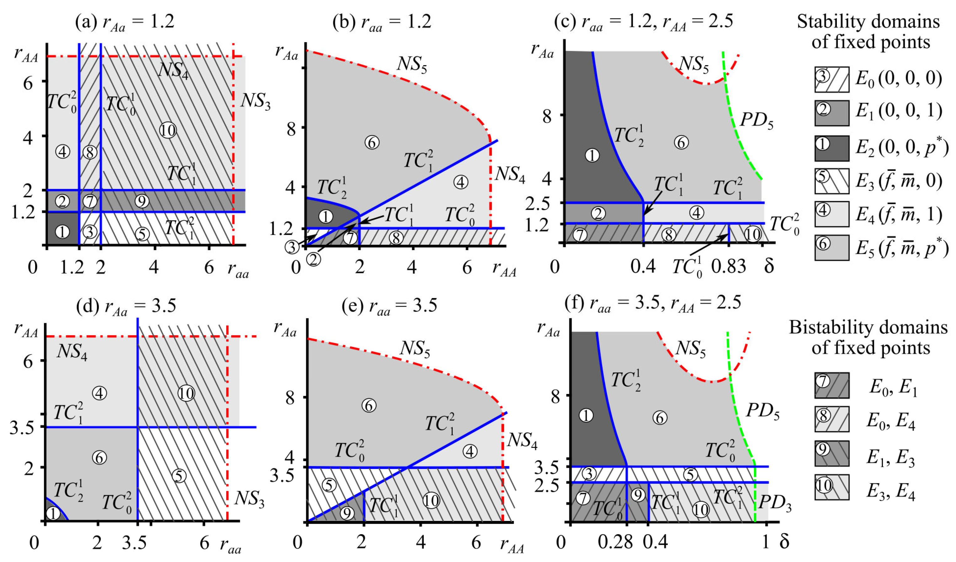
Figure 1 shows the stability domains of monomorphic and polymorphic solutions of system (2), with zero and non-zero numbers of females and males on the parameter plane ( ρ ,   r A A ) .
The presented parametric portraits demonstrate the possible dynamics of female and male abundances in a population, depending on the ratio of reproductive potentials of different genotypes and the intensity of ecological limitation (Figure 1). Note that the loss of stability of equilibrium solutions with non-zero abundance (i.e., E3, E4, and E5) is realized both according to the Neimark–Sacker scenario (NS) and the period doubling scenario (PD) (Table 1, Figure 1). At the same time, the genetic composition will remain constant and correspond either to monomorphism or polymorphism, depending on the ratio of reproductive potentials of the heterozygote and homozygotes.
First, let us fix the parameters of system (2) so that the reproductive potential of the heterozygote rAa takes intermediate or maximum values, i.e., during evolution with an increasing reproductive potential of genotype AA (rAA), overdominance is replaced by directional selection (Figure 1a–c). At r A a > r a a and r A a < 1 / δ , the stability domain of system (2) on the plane ( ρ ,   r A A ) consists of the stability regions of fixed points E 2 (at r A A < r A a ), E 1 (at r A a < r A A < 1 / δ ), and E 4 (at r A A > 1 / δ ), separated by bifurcation lines T C 1 2 and T C 1 1 (Figure 1a). At r A A < r A a and r a a < r A a , there is overdominance, i.e., the population is polymorphic, but due to insufficient reproduction, including due to the sex ratio, the population becomes extinct. With a further increasing reproductive potential r A A at r a a < r A a < r A A < 1 / δ , the most fecund and, therefore, the most successful genotype is AA; it displaces all others; however, its level of reproduction and the current sex ratio also lead to population extinction in the long run. If r A A > 1 / δ , then the reproductive potential of genotype AA reaches a level at which a monomorphic A population survives and successfully develops. At the same time, when crossing bifurcation boundary N S 4 , an increase in the reproductive potential of the homozygote AA (   r A A ) leads to a loss of stability of the solution E 4 according to the Neimark–Sacker scenario: the dynamics of female and male abundance switch to a quasiperiodic mode. When crossing the P D 4 boundary with increasing   r A A , the loss of stability of the fixed point E 4 occurs according to the period doubling scenario: stable oscillations of abundance arise, generated by a cascade of period doubling bifurcations. Moreover, the loss of stability of the solution E 4 according to the period doubling scenario occurs at smaller values of the ecological limitation intensity ρ and, according to the Neimark–Sacker scenario, at higher values of ρ .
An increase in the reproductive potential of the heterozygote r A a ( r A a > 1 / δ ) leads to the fact that the stability region of system (2) on the ( ρ ,   r A A ) plane is formed by the stability areas of solutions E 2 (at r A A ( δ r A a 2 2 r A a + r a a ) / ( r a a δ 1 ) ), E 5 (at ( δ r A a 2 2 r A a + r a a ) / ( r a a δ 1 ) < r A A < r A a ), and E 4 (at r A A > r A a ), separated by bifurcation lines T C 2 1 and T C 1 2 (Figure 1b). In this case, with the increasing reproductive potential of genotype AA during evolution, monomorphism replaces polymorphism. Moreover, at r A A ( δ r A a 2 2 r A a + r a a ) / ( r a a δ 1 ) , the polymorphic population becomes extinct due to insufficient reproduction.
Higher r A a values expand the stability domain of the polymorphic solution E 5 (Figure 1c). At the same time, with increasing r A a values, the stability region of the monomorphic fixed point E 4 narrows due to the shift of the transcritical bifurcation line (Figure 1a–c). The boundaries corresponding to the period doubling ( P D 4 ) and Neimark–Sacker ( N S 4 ) bifurcations remain unchanged. In turn, changing the reproductive potential values of the aa homozygote in the range of 0 < r a a < r A a does not affect the type and shape of the E 4 solution stability region (Figure 1).
With the reproductive potential of the heterozygote being smaller than that of both homozygotes, the increase in the reproductive potential of genotype AA leads to the fact that a “bistability trap” replaces directional selection. The second row of Figure 1 demonstrates the bistability of monomorphic solutions. The stability region of system (2) consists of the stability regions of solutions E 0 , E 1 , and E 4 (Figure 1d); E 1 , E 3 , and E 4 (Figure 1e); and E 3 and E 4 (Figure 1f).
The bistability of monomorphic fixed points E 0 and E 1 and E 0 and E 4 takes place when the stability domains of the monomorphic A allele fixed points with zero ( E 1 ) and non-zero ( E 4 ) abundances, separated by the line r A A = 1 / δ (line T C 1 1 ), overlap with the stability region of the monomorphic a allele solution with a zero population number ( E 0 ) (Figure 1d). If the stability domains of fixed points E 1 and E 4 intersect with the stability region of equilibrium E 3 with non-zero abundance, the bistability of E 3 with E 1 and E 3 with E 4 arises, respectively (Figure 1e). The stability domain of solution E 3 in the parameter plane ( ρ ,   r A A ) is a strip parallel to the ordinate axis (Figure 1e,f). One can see that with increasing values of the parameter ρ , characterizing ecological limitation, solution E 3 can lose stability according to the period doubling scenario (via P D 3 ) and the Neimark–Sacker scenario ( N S 3 ). Figure 1e,f show that the stability areas of fixed point E 3 cover those of E 4 . One can see domains where both solutions E 3 and E 4 are simultaneously stable or unstable, or where one of them is attractive but the other is not. This indicates the bistability of monomorphic solutions when the equilibrium dynamics of the population size with the aa genotype can coexist with periodic or quasiperiodic fluctuations in the population with genotype AA or vice versa.
Note that the picture of dynamic behavior on the parameter plane ( ρ ,   r a a ) is similar to ( ρ ,   r A A ) , since the solutions of system (2) are symmetric to r A A and r a a .

5. Type of Selection and Dynamics of System (2)

The type of selection and, accordingly, the dynamics of the genetic composition in system (2) depend on the ratio of reproductive potentials of the heterozygote and homozygotes r A A , r A a , and r a a (Figure 2). Let us consider this in more detail.

5.1. Increased Reproductive Potential of Heterozygotes

With r A a > max ( r A A , r a a ) , the population maintains stable polymorphism at the equilibrium allele A frequency, i.e., p ¯ A = p * . At the same time, the monomorphic solutions p ¯ A = 0 and p ¯ A = 1 exist but are unstable. In this case, there is selection favoring heterozygotes, known as a balancing selection (or heterozygote advantage) [87].
In system (2), there can be two polymorphic fixed points with zero ( E 2 ) and non-zero ( E 5 ) female and male abundances. The polymorphic point with a non-zero population abundance E 5 is stable if, in addition to the condition of a selective advantage of heterozygotes, the following ratio holds: r A a > r A a * = 1 + ( r A A δ 1 ) ( r a a δ 1 ) / δ (region 6 in Figure 2). However, at r A a < r A a * , the polymorphic fixed point with a zero population size E 2 becomes stable (region 1 in Figure 2).
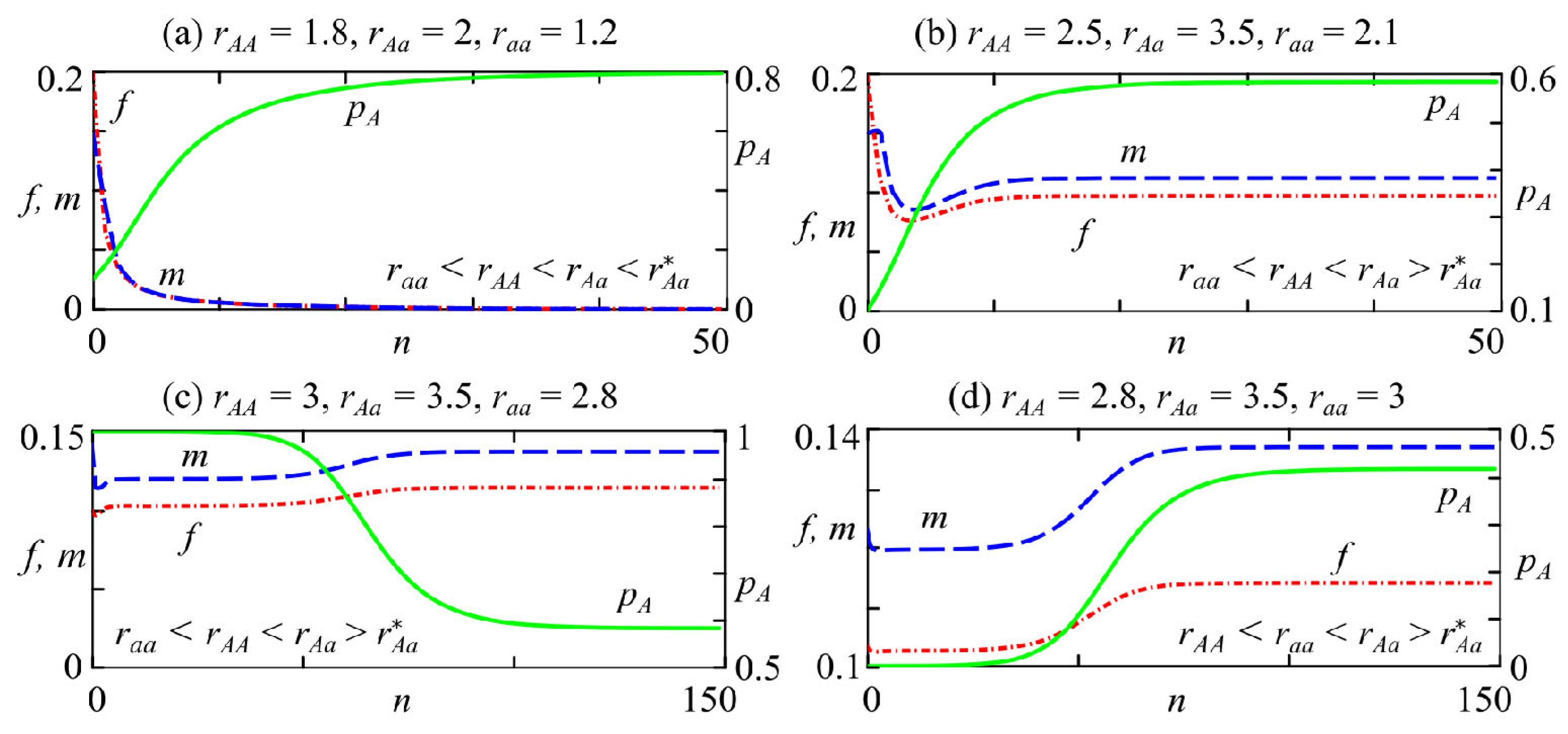
At low reproductive potential values of homozygotes compared with heterozygotes, i.e., r A A < r A a and r a a < r A a , from any polimorphic initial condition, the allele A frequency monotonically tends to the polymorphic equilibrium p ¯ A = p * with zero (at r A a < r A a * , Figure 3a) or non-zero (at r A a > r A a * , Figure 3b) female f and male m abundances. Note that at r A a < r A a * , the population maintains its genetic variety, but the growth rate is such that it eventually goes extinct. Accordingly, the level of successful reproduction at which the population survives depends not only on the genotype fitness but also on the secondary sex ratio (δ).
Consider a situation where the initial allele A frequency in the population is close to 1 at r a a < r A A < r A a (Figure 3c). This arises when genotype AA becomes predominant in a population with two sexes due to an external factor’s influence and the number of individuals of other genotypes is too small. However, over time, while maintaining the increased reproductive potential of heterozygous individuals in the population, stable polymorphism is established (Figure 3c). Consequently, the other genotypes differing from AA can appear in the next generation under favorable conditions. A similar situation arises when the initial A allele frequency is close to 0 and r A A < r a a < r A a , as shown in Figure 3d.

5.2. Intermediate Values of the Reproductive Potential of Heterozygotes

0 < r a a < r A a < r A A or 0 < r A A < r A a < r a a , corresponding to so-called driving selection, lead to the establishment of monomorphism with more fitted alleles [87].
At 0 < r a a < r A a < r A A , the selection results in allele A fixation with allele a displacement. In this case, two monomorphic equilibria of the population genetic structure exist; one of them, p ¯ A = 0 , is unstable, and the other, p ¯ A = 1 , is stable.
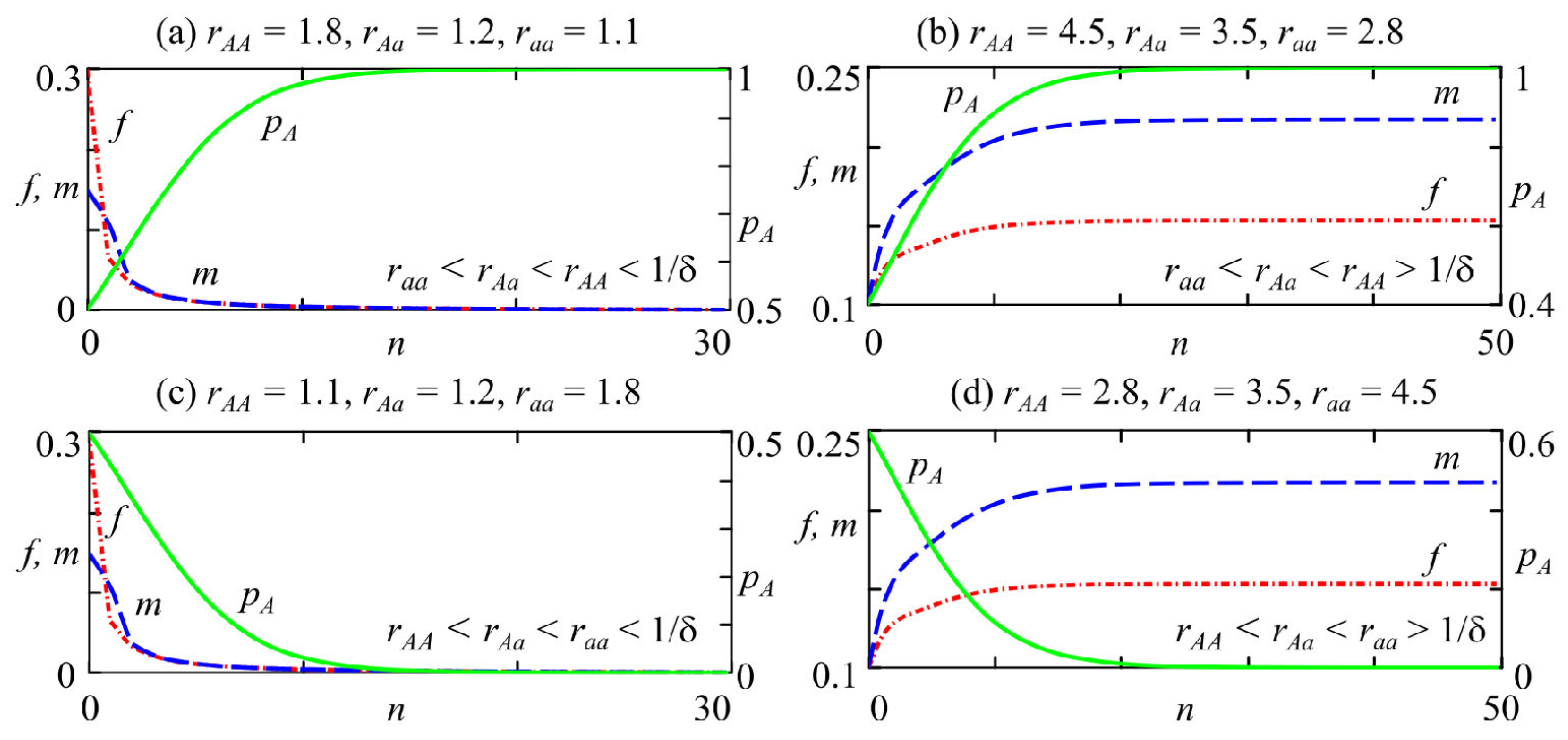
The bifurcation line r A A = 1 / δ separates the stability domains of monomorphic fixed points with zero ( E 1 ) and non-zero ( E 4 ) densities of females and males with AA genotypes (regions 2 and 4 in Figure 2). With r A A < 1 / δ , the monomorphic allele A fixed point with a zero population size is stable (region 2 in Figure 2). If r A A > 1 / δ , then E 4 with non-zero density is stable (area 4 in Figure 2). For any pA value in the range of 0 < p A < 1 , the allele A frequency monotonically increases and tends to unity. Consequently, only individuals with the AA genotype survive in the population, while individuals with the aa and Aa genotypes become extinct. The population size tends to either zero with r A A < 1 / δ (Figure 4a) or a non-zero value with r A A > 1 / δ (Figure 4b).
With 0 < r A A < r A a < r a a , allele a is fixed, and allele A is eliminated for any polymorphic initial condition. In the case of r a a < 1 / δ , the point E 0 , corresponding to the zero monomorphic fixed point with respect to allele a, is attractive (region 3 in Figure 2). If r a a > 1 / δ , then point E 3 is stable, which corresponds to a monomorphic allele a population with non-zero size (area 5 in Figure 2). Consequently, at 0 < r A A < r A a < r a a , for any non-zero initial condition, the frequency of allele A monotonically decreases to 0, and the population size tends to either zero with r a a < 1 / δ (Figure 4c) or a non-zero value with r a a > 1 / δ (Figure 4d).

5.3. Reduced Reproductive Potential of Heterozygotes

r A a < min ( r A A , r a a ) leads to the bistability of monomorphic states when two extreme genetic structures in the population are stable. Disruptive selection, also known as destructive selection, promotes the survival of extreme genotypes and the elimination of intermediate ones from generation to generation [87].
With a disruptive type of selection, a non-trivial polymorphic fixed point p ¯ A = p * exists, but it is unstable. There are two stable states in which the allele frequency is either p ¯ A = 0 or p ¯ A = 1 . Which fixed point is attractive depends on the initial genetic structure of the population. If the allele A frequency is smaller than p * in the initial generation, then it drops to 0 ( p A 0 ). If the initial value p A ( 0 ) is in the range of p * < p A ( 0 ) < 1 , then the allele A frequency increases to 1 ( p A 1 ). Consequently, with a reduced reproductive potential in heterozygotes, the result of selection is determined by the values of the reproductive potentials of homozygotes and heterozygotes and by the initial genetic structure of populations.
System (2) reveals four variants of bistability for fixed points.
Variant 1: The bistability of fixed points E 0 and E 1 , corresponding to monomorphic populations with aa and AA genotypes, respectively, with zero group sizes of females and males. The simultaneous coexistence of these stable fixed points occurs when the following conditions hold: 0 < r A a < r A A r a a < 1 / δ or 0 < r A a < r a a r A A < 1 / δ for system (2) parameters (area 7 in Figure 2). Consequently, depending on the allele A frequency in the initial generation, selection leads to either allele A fixation with p * < p A ( 0 ) < 1 or its displacement with 0 < p A ( 0 ) < p * . In both cases, the population size decreases until it becomes extinct.
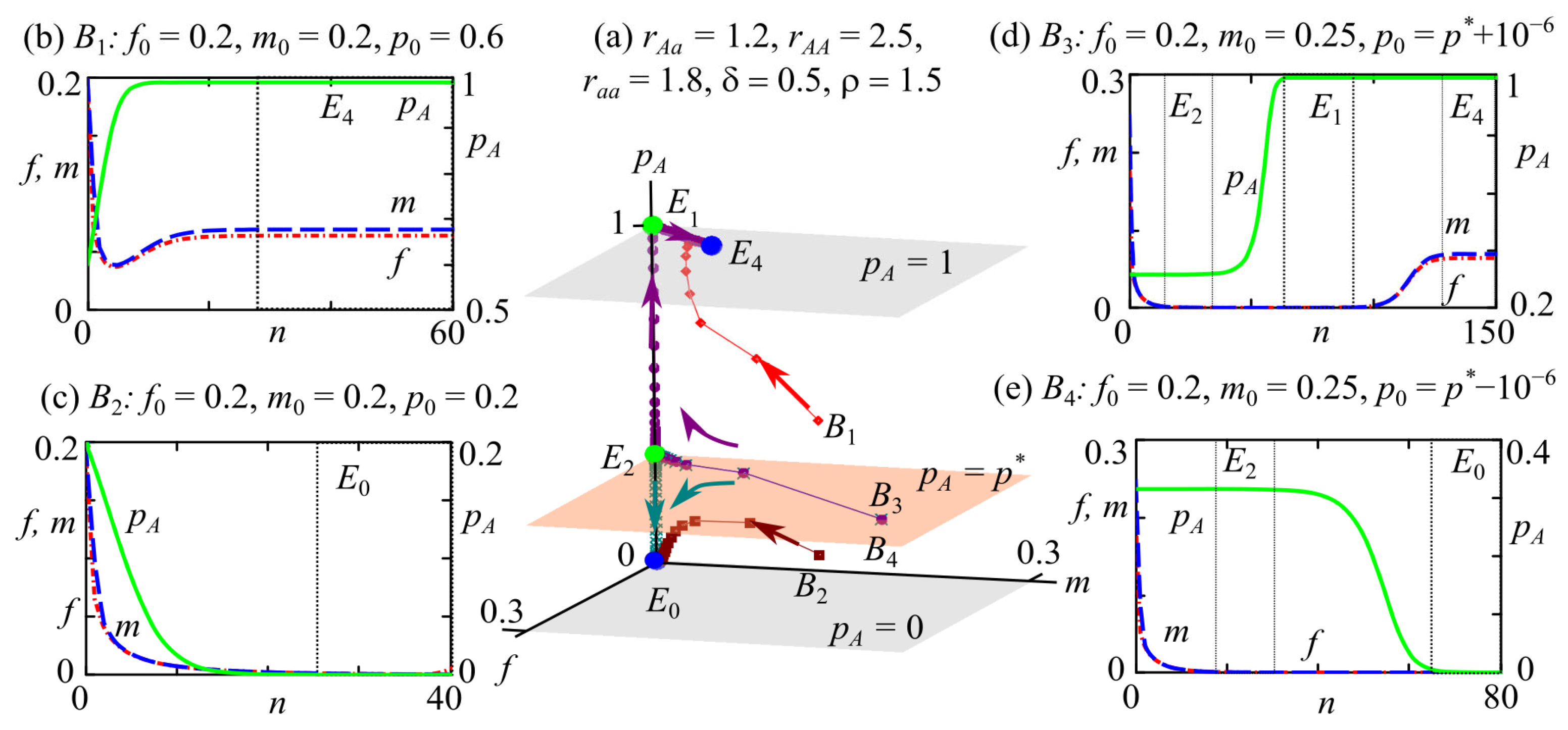
Variant 2: The bistability of fixed point E 0 , corresponding to a zero monomorphic aa population and E 4 with an AA genotype population of non-zero size. The bistability of these solutions exists at 0 < r A a < r a a < 1 / δ < r A A (region 8 in Figure 2a–c). For example, Figure 5 shows a trajectory and surface p A ( f , m ) = p * in the phase space of system (2). The surface p A ( f , m ) = p * , denoted as p A = p * in Figure 5a, is self-mapped, because all trajectories whose initial points are on this surface belong to it. Obviously, polymorphic fixed points E 2 ( 0 ,   0 ,   p * ) and E 5 ( f ¯ ,   m ¯ ,   p * ) , where 0 < p * < 1 , belong to this surface.
With the reduced reproductive potential of heterozygotes, p A ( f , m ) = p * is a separatrix surface dividing the phase space of system (2) into two attraction basins of stable monomorphic fixed points. If the initial frequency of allele A p A ( 0 ) is in the range of p * < p A ( 0 ) < 1 (point B 1 in Figure 5a), then all trajectories move away from this surface and tend to the monomorphic allele A fixed point with a non-zero population size (Figure 5a,b). At 0 < p A ( 0 ) < p * (the initial point B 2 in Figure 5a), the trajectories tend to the monomorphic allele a solution with a zero population size (Figure 5a,c). The allele A frequency monotonically changes and corresponds to logistic growth (Figure 5b) or decline (Figure 5c).
In the case of the presence of unstable fixed points E 1 and E 2 , the transition process to one of the monomorphic states E 4 or E 0 changes if the allele A frequency in the initial generation is close to the polymorphic equilibrium value p * .
When the value p A ( 0 ) is within the range of p * < p A ( 0 ) < 1 and close to the separatrix surface p A ( f , m ) = p * , for example, the initial point B 3 in Figure 5a, the system (2) trajectory, initially approaches a polymorphic fixed point E 2 and then tends to a zero monomorphic solution E 1 and subsequently achieves a monomorphic state E 4 with a non-zero population size (Figure 5a,d). Such dynamic behavior is the so-called “bottleneck effect”, when a catastrophic decrease in population size is caused by various reasons and, following its recovery, is accompanied by a reduction in genetic variety [53,56]. Figure 5d demonstrates that initially, the population is polymorphic; over time, its size decreases to a very small number of individuals. Because r A A > r a a > r A a , the genotype AA with the highest fitness fixes due to driving selection [85]. As a result, genetic variety diminishes, and the population will present only individuals with the genotype AA. Over time, the population size increases again, but genetic variety is not restored. As depicted in Figure 5d, due to passing through a population bottleneck, the population loses genotypes Aa and aa, which have lower reproductive potential and, in this case, result in extinction in the future. This type of system behavior can be considered and interpreted as an effect of evolutionary rescue. A U-shaped curve of population size over time characterizes the process of evolutionary rescue. Initially, the population size decreases due to poor adaptation to environmental conditions, and fitness increases as adaptive alleles spread in the population [56,58].
If the allele A frequency in the initial generation is close to p A ( f , m ) = p * but smaller than the value p * (the initial point B 4 in Figure 5a, 0 < p A ( 0 ) < p * ), then all trajectories moving away from this surface tend to allele a monomorphic solution E 0 with a zero population size (Figure 5a,e). This transition is initially accompanied by a reduction in population size but without a loss of genetic variety. Over time, however, genetic impoverishment occurs in the population, resulting in the survival of only homozygous aa individuals. Such processes are critical for the population’s development, and because the reproductive potential of homozygote aa is insufficient for survival, its value is in the range r a a < 1 / δ < r A A and leads to population extinction.
Variant 3: The bistability of fixed points E 1 and E 3 when a monomorphic AA stable state with a zero population abundance coexists with a monomorphic aa solution with a non-zero population size. This bistability exists if the condition 0 < r A a < r A A < 1 / δ < r a a holds (region 9 in Figure 2a,e,f).
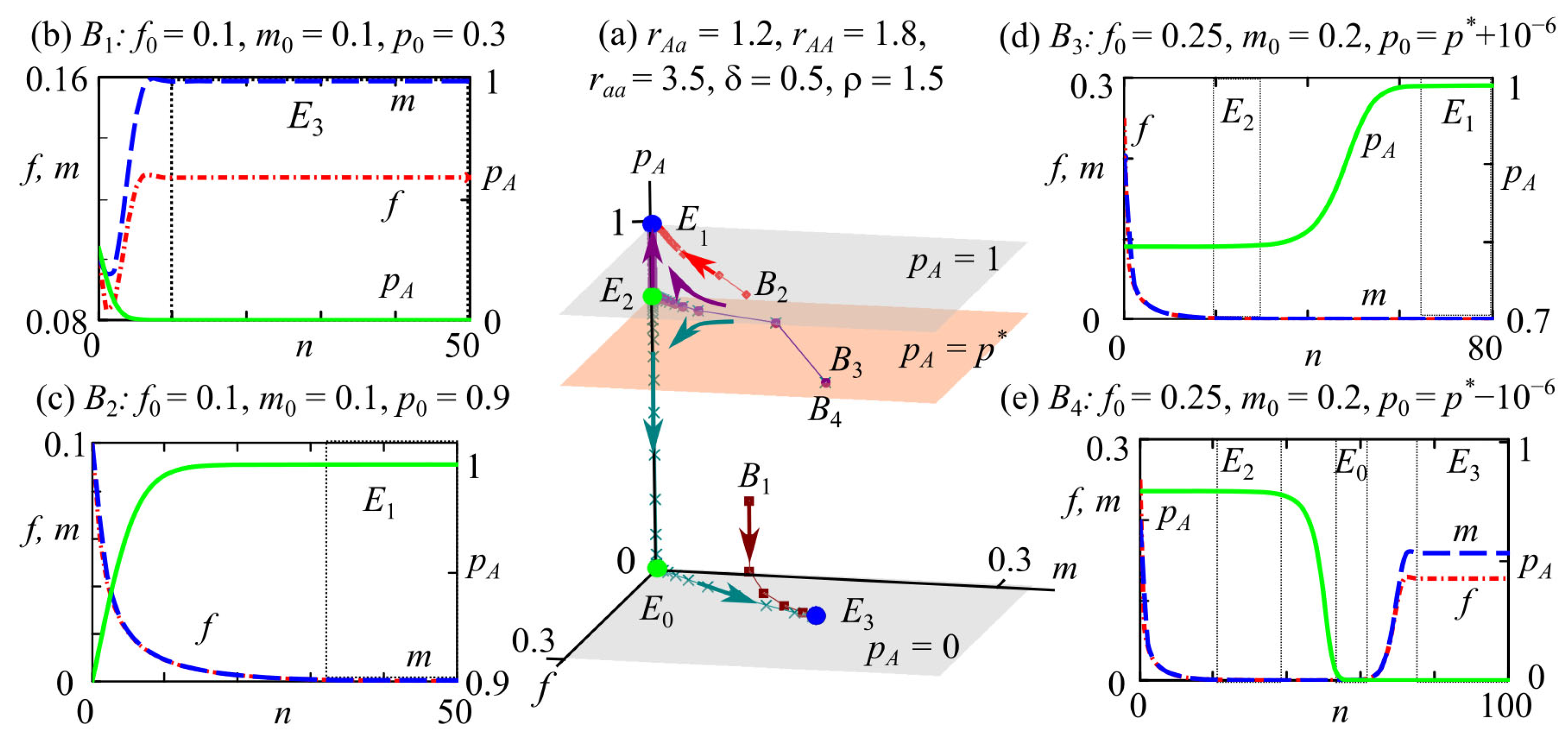
In the phase space of system (2), the attraction basins of fixed points E 1 and E 3 are bounded by surfaces p A = 1 , p A ( f , m ) = p * , and p A = 0 (Figure 6).
If the frequency of allele A in the initial generation p A ( 0 ) is in the range of 0 < p A ( 0 ) < p * , such as point B 1 in Figure 6a, then all trajectories tend to the monomorphic aa solution with a non-zero population size E 3 (Figure 6a,b). With p A ( 0 ) from the range of p * < p A ( 0 ) < 1 , for example, the starting point B 2 in Figure 6a, which is the monomorphic AA fixed point with zero abundance E 1 , is attractive (Figure 6a,c).
Similar to the previous case, if the initial allele A frequency is close to the value p * for the polymorphic fixed point, then the presence of unstable solutions E 0 and E 2 leads to non-monotonic transition processes in the system dynamics.
Figure 6a shows an example with an initial point B 3 at p A ( 0 ) = p * + 10 6 when the initial allele A frequency p A ( 0 ) is slightly higher than the polymorphic equilibrium frequency p * . We can see that at the beginning, p A tends to a value that is close to the fixed point E 2 while maintaining polymorphism (Figure 6d). Then, during evolution, allele A accumulates and displaces allele a, i.e., the population becomes monomorphic in allele A. However, the reproductive potential of AA genotype individuals is insufficient for population survival, since r A A < 1 / δ < r a a (Figure 6a,d).
With the allele A frequency in the initial generation p A ( 0 ) being slightly smaller than p * , as an example, for the starting point B 4 at p A ( 0 ) = p * 10 6 in Figure 6a, system (2) trajectories tend firstly to solution E 2 , then to point E 0 , and only after that, they reach equilibrium E 3 . Consequently, during evolution, allele a accumulates in the polymorphic population, which leads to allele A elimination (Figure 6a,e). At the same time, the numbers of females and males in the population initially decrease to a critical level, then slowly grow and reach equilibrium E 3 .
Figure 6e illustrates a U-shaped curve of the changes in the group sizes of females and males over time. Initially, the population size decreases due to the low reproductive potential of individuals with genotypes Aa and AA. During evolution, the more adaptive allele a accumulates, which leads to population size growth caused by selection and the survival of homozygous individuals with the most suitable genotype aa. Here, as in the previous cases, a temporary sharp decline in population size can be considered as passing through a bottleneck. Evolutionary rescue of the population is achieved by increasing the frequency of the existing allele a, which was initially rare. Note that if allele a was not rare, then a catastrophic reduction in population size would not have been observed (Figure 6b).
Variant 4: The bistability of fixed points E 3 and E 4 , corresponding to the coexistence of two monomorphic equilibria with non-zero group sizes of females and males. System (2) reveals this bistability if the conditions 0 < r A a < r a a < r A A , r a a > 1 / δ (domain 10 in Figure 2a,c,d), or 0 < r A a < r A A < r a a , r A A > 1 / δ (domain 10 in Figure 2a,d,f) hold.
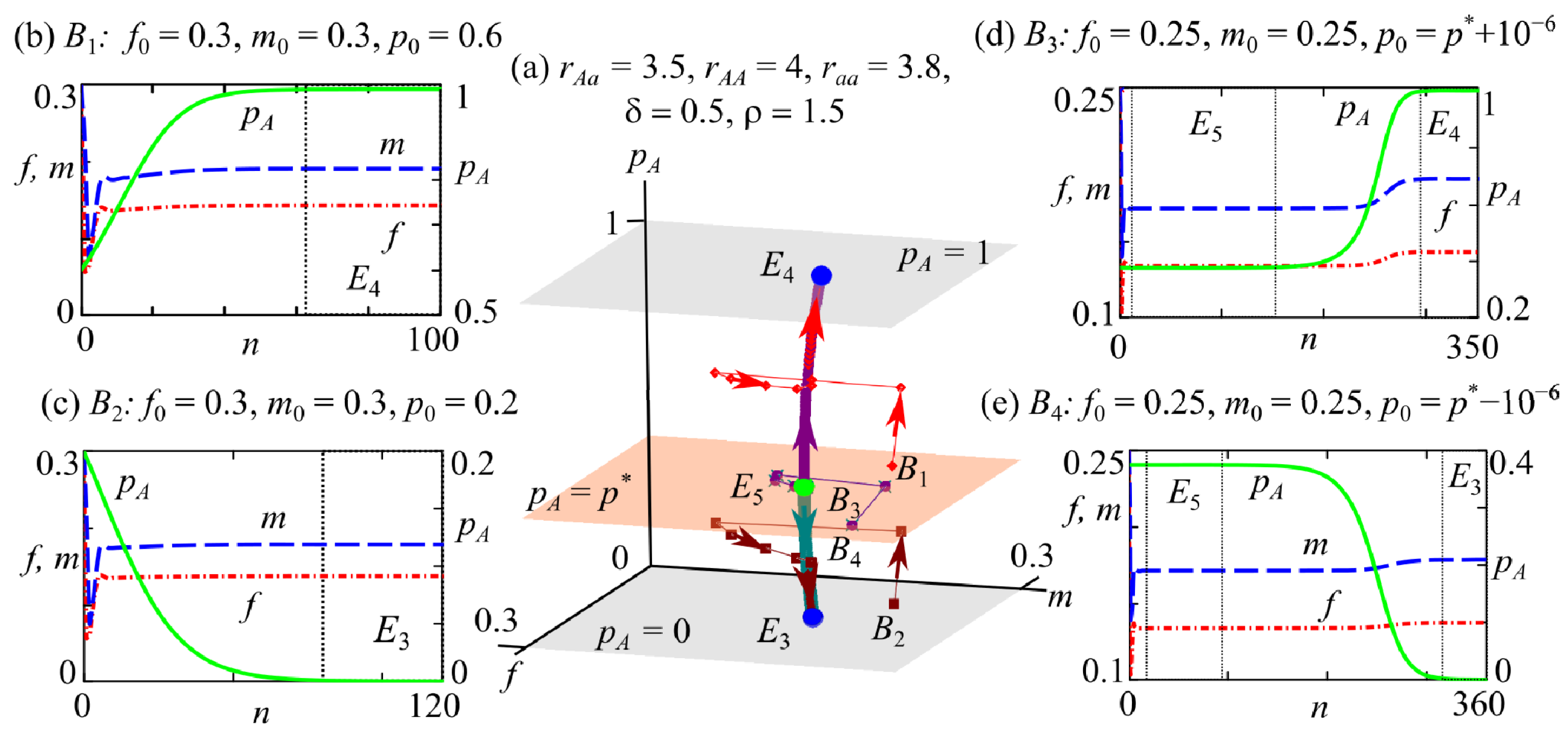
Similar to the previous cases, in the system (2) phase space, the attraction basins of fixed points E 3 and E 4 are bounded by the surfaces p A = 0 , p A ( f , m ) = p * , and p A = 1 , as shown in Figure 7a.
As in the case of the previous variant, with the initial point lying above the separatrix surface p A ( f , m ) = p * (point B 1 in Figure 7a), the population becomes monomorphic with the AA genotype during evolution (Figure 7b). If the starting point is below p * , such as B 2 in Figure 7a, then the evolution outcome is a monomorphic aa population (Figure 7c). However, if the allele A frequency in the initial generation p A ( 0 ) is close to its value p * for the polymorphic solution, such as for example the initial points B 3 and B 4 in Figure 7a, then the population can maintain polymorphism for a long time during the transition process (Figure 7d,e). Here, we observe the fixation of one of the alleles and the elimination of the other, which results in a monomorphic population (Figure 7d,e).
Thus, in this case, the outcome of evolution depends on the initial frequencies of allele A at the initial stage of population development. With p < p * , allele A will be displaced; at p > p * , it will fix. Consequently, the current genetic structure of the population determines the outcome of evolution due to occurrences of the so-called “bistability trap”, when a more promising genotype may be displaced by one with less fitness [25,26].
Above, we have considered various types of bistability of stable monomorphic solutions of system (2). Note that at higher values of the reproductive potential of genotypes, monomorphic fixed points with non-zero numbers lose stability according to the period doubling bifurcation or Neimark–Sacker scenario (Figure 1). As a result, we can observe the bistability of trivial/non-trivial stable solutions with periodic or quasiperiodic dynamics.

6. Dynamics of the Genetic Composition of the Population with Changes in the Reproductive Potential of Genotypes

This section considers the dynamics of the genetic composition of the population and the group sizes of females and males with the changing reproductive potential of individuals of different genotypes during evolution. An increase in reproductive potential can be caused, for example, by mutations when alleles with higher fitness appear. Accordingly, we assume that in a hypothetical monomorphic aa population, as a result of mutation, a new adaptive allele A0 with a higher reproductive potential arises, and its frequency gradually increases. Initially, the ratio of the reproductive potentials of homozygotes and heterozygotes is chosen so that system (2) trajectories converge to the monomorphic A0A0 solution with a zero population size (range I in Figure 8a). After 200 iterations of a monotonous increase in the allele A0 frequency and nearly fixing it in the population, a new allele A1 with a higher reproductive potential appears due to another mutation while maintaining a near-zero population size. During driving selection, the A1 allele frequency in the population monotonically grows, and allele A1 displaces the A0 allele. At the same time, the population size slowly increases, which corresponds to the tendency of the trajectory to a non-zero stationary state (range II in Figure 8a).
The population size curves for females and males are U-shaped (intervals I and II in Figure 8a), which corresponds to the evolutionary rescue of the population due to the increase in the frequency of a new allele A1 with a higher reproductive potential that appears due to a mutation.
Furthermore, when the “good” allele A1 becomes almost fixed and its frequency is close to p A 1 = 0.99 , a new better allele A2 with a higher reproductive potential of homozygote r A 2 A 2 appears. With the emergence of this superior allele A2, the current equilibrium population sizes of females and males approach a higher level (interval III in Figure 8a). As allele A2 becomes more prevalent, it replaces allele A1, and a new allele A3 emerges, which has even higher fitness (interval IV in Figure 8a). Thus, the mutations and driving selection lead to a series of transitions, resulting in the growth of the average reproductive potential of the population over time (Figure 8a).
Figure 8b illustrates the process of the emergence of “good” alleles with reproductive potential whose values do not result in population extinction. Similar to the previous case, the arising mutants (alleles) compared with the wild species are assumed to have adaptive superiority. At driving natural selection, new alleles with higher fitness become fixed. If individuals with a new allele are superior in fitness to those with the wild allele, the new allele frequency in the population will gradually increase (Figure 8b). This process corresponds to the mechanism of allele fixation [87]. If the emergence of new alleles continues, this leads to fluctuations in population size over time due to the increase in the average reproductive potential of genotypes and density-dependent survival regulation (Figure 8b).
Consequently, genotypes with a higher reproductive potential become gradually fixed in the population, which leads to an evolutionary increase in their average reproductive potential. This results in an increase in the stationary numbers of females and males, as well as in bifurcations of the stability loss for current population equilibrium with an oscillation emergence.

7. Discussion

This study proposed and investigated the evolutionary dynamics model of a limited population that is structured by sex. We assumed genetic variety in the population concerning reproductive potential, controlled by a single autosomal diallelic locus. For the proposed model, we found monomorphic and polymorphic fixed points with conditions for their existence and stability (Table 1). The system is shown to reveal periodic and quasiperiodic oscillations, caused by the occurrence of a period doubling bifurcation and a Neimark–Sacker one (Figure 1). The scenario of system stability loss depends on the intensity of ecological limitations. However, the evolutionary results are always the same: with increasing genotypes’ reproductive potentials r A A , r A a , and r a a , the population dynamics become more irregular and complex.
We classified regions with different dynamics of population size and genetic composition (Figure 2). The outcomes of selection by reproductive potential values (F-selection) in ecologically limited populations with sex or stage structure [20,21] are shown to have no difference from those of Fishers’ fitnesses in unlimited ones. As expected, the condition for maintaining a stable polymorphism in a population is r A a > max ( r A A , r a a ) , which corresponds to the highest value of the heterozygote reproductive potential (Figure 3). When r a a < r A a < r A A or r A A < r A a < r a a , intermediate values of heterozygote fitness lead to a monomorphism for alleles with greater reproductive potential (Figure 4). The level of successful reproduction at which a population with two sexes can survive and grow depends on the ratio of reproductive potentials of the genotypes and the secondary sex ratio δ , which determines the proportion of female newborns.
With the reduced reproductive potential of heterozygotes r A a < min ( r A A , r a a ) , the proposed model reveals bistability (Figure 5, Figure 6 and Figure 7). This bistability corresponds to the coexistence of both monomorphic fixed points, when the initial sex ratio and allele frequencies determine the genotype that will be fixed in the population. This scenario is a so-called “bistability trap”, which means that a higher-fitness genotype cannot displace those with lower fitness. However, a drop in population size due to external environmental factors leads to random processes, known as “passage through a bottleneck”, that can result in fluctuations in the genetic composition and a “shift” of the population from one monomorphic state to another one with more fitness, for which population dynamics destabilize.
In contrast to previously studied eco-evolutionary population models with a stage structure [20,21], the proposed model can show several types of bistability due to considering sexual dimorphism and, as a result, the secondary sex ratio. Depending on the initial allele frequencies and the sex ratio, the population may either become extinct or survive with the fixation of one of the alleles, as different monomorphic fixed points may coexist (Figure 5 and Figure 6). For example, one fixed point has a zero population size, while the other has non-zero numbers of males and females. This means that some initial conditions can increase the frequency of lower-fitness alleles, leading to population extinction due to a decrease in the growth rate (Figure 5c,e and Figure 6c,d). There are also initial conditions that can increase the frequency of an allele with a higher reproductive potential, for which, depending on the values of specific demographic parameters, the population size may show an equilibrium tendency or fluctuations (Figure 5b,d and Figure 6b,e). In this case, the variation in the current genetic composition of the population due to the influence of unaccounted environmental factors can change the “initial conditions” and, thus, the direction of evolution. Consequently, some external factors may lead to the extinction of a successfully developing population or its gradual recovery after a significant decline in its number.
The model study shows that, in the case of bottlenecks in population size, its genetic variety decreases, and if an allele with a higher reproductive potential is fixed, then the other one is eliminated (Figure 5d and Figure 6e). As a result, the population recovers because the genotype is cleared due to the removal of the low-fitness allele.
The population recovery in the proposed system illustrates so-called “evolutionary rescue” [56,57,58], where a population facing the threat of extinction is capable of adapting by increasing the frequency of alleles with higher fitness to prevent extinction. Figure 5d and Figure 6e demonstrate the case of evolutionary rescue when the population recovers due to the accumulation of initially rare alleles with a higher reproductive potential. The example of the regeneration of the natural population of the northern elephant seal, Mirounga angustirostris, allows us to suggest that this population has survived without fundamental changes, despite significant genetic diversity loss due to passing through a bottleneck [88]. However, strategies for population conservation and management require careful consideration of the possible consequences of the application of the developed measures.
Theoretical studies of the dynamics of structured populations with density-dependent regulation have shown that an increase in birth rate and survival parameters leads to more complex population dynamics [81,82,83,89]. Considering a genetic structure in the model of an ecologically limited sex-structured population, similar to those with a stage structure, allows us to investigate the possibilities of an evolutionary transition from equilibrium to fluctuations when an increase in the fertility of individuals occurs during evolution under the influence of natural selection. We have shown that the appearance of new alleles with a higher reproductive potential in individuals, for example due to mutations, leads to natural selection of these alleles and an evolutionary increase in the average birth rate of the population (Figure 8). However, density-dependent survival regulation with the growth of the average reproductive potential destabilizes the dynamics of the size of the female and male groups. We have shown that another scenario of evolutionary rescue occurs when the population recovers due to new alleles with a higher reproductive potential whose appearance is caused, for example, by mutations (Figure 8a). Note that the possibility of evolutionary rescue [22,23] and fluctuation emergence in limited populations [24,25,26] due to fixation of the alleles with higher fitness, whose appearance is caused by mutations, was expected, since this was previously demonstrated in dynamic models of stage-structured populations.

8. Conclusions

This study showed that an increase in the average value of the reproductive potential in a population with density-dependent regulation of survival destabilizes the dynamics of abundance of females and males. In this case, the scenario of stability loss of equilibrium via the period doubling or Neimark–Sacker bifurcations depends on the intensity of self-regulation. The genetic composition of the population, namely, monomorphic genotype fixation or coexistence of all genotypes in polymorphism, is shown to be determined by the values of the reproductive potentials of heterozygotes and homozygotes, initial conditions, and a parameter describing the ratio of newborn females to males. In particular, we found that the increased reproductive potential of heterozygotes leads to a stable polymorphism within a population. The intermediate value of the reproductive potential of heterozygotes results in a monomorphism with an allele with greater fitness. The reduced reproductive potential of heterozygotes induces bistable dynamics when the different monomorphic fixed points with zero and non-zero population sizes coexist. Thus, depending on the values of the initial allele frequencies and the parameter describing the ratio of newborn females to males, the population either becomes extinct or survives by fixing one of the alleles during evolution. In this scenario, the polymorphic state is unstable and is part of a transitional process in the dynamics to achieve one of the monomorphic states. With the coexistence of two monomorphic equilibria with zero and non-zero population sizes, the model of a population with two sexes proposed in this study reveals the possibility of bottleneck effects and evolutionary rescue. With the reduced reproductive potential of heterozygotes, the influence of environmental factors that are not considered in the model can alter the current genetic composition of the population, which can change the direction of evolution. This scenario corresponds to a situation in which a genotype with less fitness may displace a more promising form, and these processes are accompanied by passage through a bottleneck and evolutionary rescue. As a result, external factor influence can lead to the extinction of a successful developing population or a gradual population recovery after a noticeable decline in its abundance. This model reveals two variants of evolutionary rescue: when the population recovers due to rare alleles with higher fitness in disruptive selection or the emergence of new alleles caused by mutations in driving selection.

Author Contributions

Conceptualization, E.F. and O.Z.; investigation, O.R.; writing—original draft preparation, O.R. and G.N.; writing—review and editing, G.N., E.F. and O.Z. All authors have read and agreed to the published version of the manuscript.

Funding

This work was carried out within the framework of the state targets of the Institute for Complex Analysis of Regional Problems of the Far Eastern Branch of the Russian Academy of Sciences.

Data Availability Statement

Data are contained within the article.

Conflicts of Interest

The authors declare no conflict of interest.

Appendix A

Appendix A.1. Dynamic Equations of Allele Frequencies in a Population with a Sex Structure and Non-Overlapping Generations under Natural Selection

  • For deriving such a model, let us consider a breeding scheme with the following assumptions [35]: The trait is located on an autosome, which means that both parents determine the genotype of the offspring.
  • The production of gametes of all genotypes is assumed to be equal in the male (gfij = g2) and female (gmij = g1) part of the population, i.e., males and females may have different production gametes, but within one sex, all genotypes have the same one.
  • Gene frequencies in the male and female parts of the population may differ.
Table A1. Breeding scheme in a two-sex population that is subject to natural selection, panmixia, and Mendelian inheritance.
The n-th Generation
FemalesMales
GenotypesAAAaaaAAAaaa
Genotype frequenciespAApAapaaqAAqAaqaa
The (n + 1)th Generation
GametesAaAa
Gamete frequenciespA~
pAA+ pAa/2
pa~
paa+ pAa/2
qA~
qAA+ qAa/2
qa~
qaa+ qAa/2
ZygotesAAAaaa
FitnesseswAAwAawaavAAvAavaa
Zygote frequenciespAA, qAA ~ pAqApAa, qAa ~ pAqa + paqApaa, qaa ~ paqa
Here, wij is the fitness of female genotype ij (i and j can take values A or a), defined as the average number of eggs produced per newborn female of the corresponding genotype to later become the next generation of zygotes; vij is the fitness of male genotype ij, defined as the average number of spermatozoids produced per newborn male of the corresponding genotype to later become the next generation of zygotes.
The breeding scheme (Table A1) allows us to derive dynamic equations considering natural selection. The frequency (or share) of living offspring with AA genotypes from mothers with AA or Aa genotypes (and fathers with the same genotypes) is as follows:
W(n)pAA(n + 1) = wAA (pAA(n) + pAa(n)/2)(qAA(n) + qAa(n)/2),
where W(n) is a multiplier that maintains the following equality: pAA(n + 1) + pAa(n + 1) + paa(n + 1) = 1.
By analogy, for males:
H(n)qAA(n + 1) = vAA (pAA(n) + pAa(n)/2)(qAA(n) + qAa(n)/2),
where H(n) is a multiplier that maintains the following equality: qAA(n + 1) + qAa(n + 1) + qaa(n + 1) = 1.
Similarly, the frequency (or share) of living offspring with Aa genotypes that received an A allele from the mother and an a allele from the father and vice versa is as follows:
W(n)pAa(n + 1) = wAa(pAA(n) + pAa(n)/2)(qaa(n) + qAa(n)/2) + wAa (paa(n) + pAa(n)/2)(qAA(n) + qAa(n)/2),
H(n)qAa(n + 1) = vAa(pAA(n) + pAa(n)/2)(qaa(n) + qAa(n)/2) + wAa (paa(n) + pAa(n)/2)(qAA(n) + qAa(n)/2).
Finally, the frequency (or share) of living offspring with aa genotype from mothers with Aa or aa genotypes (and fathers with the same genotypes) is as follows:
W(n)paa(n + 1) = waa(paa(n) + pAa(n)/2)(qaa(n) + qAa(n)/2)
H(n)qaa(n + 1) = vaa(paa(n) + pAa(n)/2)(qaa(n) + qAa(n)/2)
Summing three equations for the female and male parts of the population separately and taking into account the equalities pAA(n + 1) + pAa(n + 1) + paa(n + 1) = 1 and qAA(n + 1) + qAa(n + 1) + qaa(n + 1) = 1, as well as those connecting the frequencies of genes and genotypes {pi(n) = pii(n) + pij(n)/2, qi(n) = qii(n) + qij(n)/2}, we obtain the multipliers or the mean fitnesses for each sex:
W(n) = wAApA(n)qA(n) + wAa(pA(n)qa(n) + pa(n)qA(n)) + waapa(n)qa(n),
H(n) = vAApA(n)qA(n) + vAa(pA(n)qa(n) + pa(n)qA(n)) + vaapa(n)qa(n).
Then, summing Equations (A1) and (A3) and Equations (A3) and (A5), we obtain the following dynamic equations for the allele frequencies:
pA(n + 1) = (wAA pA(n)qA(n) + wAapA(n)qa(n)/2 + wAapa(n)qA(n)/2)/W(n),
qA(n + 1) = (vAA pA(n)qA(n) + vAapA(n)qa(n)/2 + vAapa(n)qA(n)/2)/H(n).
F (F ≥ 0) and M (M ≥ 0) are female and male abundances, respectively; p A ( n ) ( 0 p A 1 ) is the frequency of allele A in the n-th generation.
Let F(n) and M(n) denote female and male abundances in the n-th breeding season, respectively; then, F(n + 1) = W(n)F(n) and M(n + 1) = H(n)M(n).

Appendix A.2. Population Dynamics in a Case When the Birth Rate of a Population Is Determined Genetically: A Trait Is Not Sex-Limited

Let us consider a dynamic model for a population with sex and age structures [83]. Let F(n) and M(n) denote female and male abundances in the n-th breeding season, respectively, while P(n) is the progeny abundance; then, the dynamic equations are the following:
P(n + 1) = ac(F(n), M(n)),
F(n + 1) = δψ1P(n) + s F(n),
M(n + 1) = (1 − δ)ψ2P(n) + v M(n),
where a is the birth rate (average number of offspring per single mating pair), c(F(n), M(n)) is the mating function (the pair formation function), δ is the proportion of newborn females, ψ1 and ψ2 are survival rates of immature individuals, and s and v are survival rates of mature males and females, respectively. Survival rates linearly depend on the progeny and abundances of mature males and females: ψ1 = ψ1 (P, F, M), ψ2 = ψ2(P, F, M).
We assume that the birth rate is only determined by female abundance, because male abundance is enough for breeding. Therefore, the mating function has the following form: c(F(n), M(n)) = F(n). In female dominance, offspring of both sexes are born in a fixed proportion to the number of females at time n.
Therefore, for a population with non-overlapping generations, the model takes the following form:
F(n + 1) = δ r F(n) w1(F(n), M(n))
M(n + 1) = (1 − δ) r F(n) w2(F(n), M(n)).
The wij and vij coefficients are expected to be functions of female and male abundances. Let wij = rij·δ·w1(M(n), F(n)), vij = rij·(1 − δ)·w2(M(n), F(n)), where rij are the coefficients equivalent to the relative fertility rates of females and males, respectively, and functions w1 and w2 are equal for all genotypes, which holds for F selection.
Taking this into account, one can note that the genetic composition is the same in the male and female parts of the population:
W(n) = δ (rAApA(n)qA(n) + rAa(pA(n)qa(n) + pa(n)qA(n)) + raapa(n)qa(n)),
H(n) = (1 − δ)(rAApA(n)qA(n) + rAa(pA(n)qa(n) + pa(n)qA(n)) + raapa(n)qa(n)),
W(n)/δ = H(n)/(1 − δ),
pA(n + 1) = δ (rAA pA(n)qA(n) + rAapA(n)qa(n)/2 + rAapa(n)qA(n)/2)/W(n),
qA(n + 1) = (1 − δ)(rAA pA(n)qA(n) + rAapA(n)qa(n)/2 + rAapa(n)qA(n)/2)/H(n),
pA(n + 1) = qA(n + 1).
Note that even when in the initial state the genetic composition in the male and female parts of the population differs q(0) ≠ p(0), after the first crossing, it will equalize in both parts of the population (this can be seen from the equations above when substituting n = 0).
Therefore, one can use a single equation to describe the dynamics of allele frequency in a population (pA(n)). Let us write the dynamic equations in their final form:
F(n + 1) = δ r(n) F(n) w1(F(n), M(n)),
M(n + 1) = (1 − δ) r(n) F(n) w2(F(n), M(n)),
pA(n + 1) = pA(n) (rAA pA(n) + rAa(1 − pA(n))/r(n),
where r(n) = rAApA2(n) +2rAapA(n)(1 − pA(n)) + raa(1 − pA(n))2(n).

References

  1. Darwin, C. On the Origin of Species; John Murray: London, UK, 1859. [Google Scholar]
  2. Fisher, R.A. The Genetical Theory of Natural Selection; Clarendon Press: Oxford, UK, 1930. [Google Scholar]
  3. Wright, S. The genetical theory of natural selection: A review. J. Hered. 1930, 21, 340–356. [Google Scholar] [CrossRef]
  4. Haldane, J.B.S. The Causes of Evolution; Longman Green: London, UK, 1932. [Google Scholar]
  5. Chetverikov, S.S. About some moments of evolutionary process from the point of view of contemporary genetics. Zhurnal Eksp. Biol. 1926, 2, 3–54. (In Russian) [Google Scholar]
  6. Verhulst, P.F. Deuxième Mémoire sur la loi d’Accroissement de la Population; Mémoires de l’Académie Royale des Sciences, des Lettres et des Beaux-Arts de Belgique; Hayez: Bruxelles, Belgium, 1847; Volume 20, pp. 1–32. [Google Scholar]
  7. Volterra, V. Variations and fluctuations of the number of individuals in animal species living together. ICES J. Mar. Sci. 1928, 3, 3–51. [Google Scholar] [CrossRef]
  8. Gauze, G.F. Analysis of struggle for survival in mixed populations. Zool. Zhurnal 1935, 14, 243–270. [Google Scholar]
  9. Thompson, J.N. Rapid evolution as an ecological process. Trends Ecol. Evol. 1998, 13, 329–332. [Google Scholar] [CrossRef] [PubMed]
  10. Duffy, M.A.; Sivars-Becker, L. Rapid evolution and ecological host-parasite dynamics. Ecol. Lett. 2007, 10, 44–53. [Google Scholar] [CrossRef] [PubMed]
  11. Ellner, S.P.; Geber, M.A.; Hairston, N.G. Does rapid evolution matter? Measuring the rate of contemporary evolution and its impacts on ecological dynamics. Ecol. Lett. 2011, 14, 603–614. [Google Scholar] [CrossRef] [PubMed]
  12. Greenman, J.V.; Benton, T.G.; Boots, M.; White, A.R. The evolution of oscillatory behavior in age-structured species. Am. Nat. 2005, 166, 68–78. [Google Scholar] [CrossRef]
  13. Kausrud, K.L.; Mysterud, A.; Steen, H.; Vik, J.O.; Østbye, E.; Cazelles, B.; Framstad, E.; Eikeset, A.M.; Mysterud, I.; Solhøy, T.; et al. Linking climate change to lemming cycles. Nature 2008, 456, 93–97. [Google Scholar] [CrossRef]
  14. Barraquand, F.; Louca, S.; Abbott, K.C.; Cobbold, C.A.; Cordoleani, F.; DeAngelis, D.L.; Elderd, B.D.; Fox, J.W.; Greenwood, P.; Hilker, F.M.; et al. Moving forward in circles: Challenges and opportunities in modelling population cycles. Ecol. Lett. 2017, 20, 1074–1092. [Google Scholar] [CrossRef]
  15. Pimentel, D. Population regulation and genetic feedback. Science 1968, 159, 1432–1437. [Google Scholar] [CrossRef]
  16. Roughgarden, J. Density-dependent natural selection. Ecology 1971, 52, 453–468. [Google Scholar] [CrossRef]
  17. Charlesworth, B. Selection in density-regulated populations. Ecology 1971, 52, 469–474. [Google Scholar] [CrossRef]
  18. Frisman, E.; Shapiro, A. Fluctuations in the Size of Isolated Single-Species Populations and Natural Selection. Biom. J. 1982, 24, 531–542. [Google Scholar] [CrossRef]
  19. Frisman, E.Y.; Zhdanova, O.L. Evolutionary transition to complex population dynamic patterns in a two-age population. Russ. J. Genet. 2009, 45, 1124–1133. [Google Scholar] [CrossRef]
  20. Tyutyunov, Y.; Zhadanovskaya, E.; Bourguet, D.; Arditi, R. Landscape refuges delay resistance of the European corn borer to Bt-maize: A demo-genetic dynamic model. Theor. Popul. Biol. 2008, 74, 138–146. [Google Scholar] [CrossRef]
  21. Tyutyunov, Y.V.; Kovalev, O.V.; Titova, L.I. Spatial demogenetic model for studying phenomena observed upon introduction of the ragweed leaf beetle in the South of Russia. Math. Model. Nat. Phenom. 2013, 8, 80–95. [Google Scholar] [CrossRef]
  22. De Vries, C.; Caswell, H. Selection in two-sex stage-structured populations: Genetics, demography, and polymorphism. Theor. Popul. Biol. 2019, 130, 160–169. [Google Scholar] [CrossRef]
  23. De Vries, C.; Caswell, H. Stage-structured evolutionary demography: Linking life histories, population genetics, and ecological dynamics. Am. Nat. 2019, 193, 545–559. [Google Scholar] [CrossRef]
  24. De Vries, C.; Desharnais, R.A.; Caswell, H. A matrix model for density-dependent selection in stage-classified populations, with application to pesticide resistance in Tribolium. Ecol. Model. 2020, 416, 108875. [Google Scholar] [CrossRef]
  25. Neverova, G.P.; Zhdanova, O.L.; Frisman, E.Y. Effects of natural selection by fertility on the evolution of the dynamic modes of population number: Bistability and multistability. Nonlinear Dyn. 2020, 101, 687–709. [Google Scholar] [CrossRef]
  26. Neverova, G.P.; Frisman, E.Y. Dynamic modes of population size and its genetic structure for species with nonoverlapping generations and stage development. Commun. Nonlinear Sci. Numer. Simul. 2021, 94, 105554. [Google Scholar] [CrossRef]
  27. Tyutyunov, Y.V. Spatial Demo-Genetic Predator–Prey Model for Studying Natural Selection of Traits Enhancing Consumer Motility. Mathematics 2023, 11, 3378. [Google Scholar] [CrossRef]
  28. Wright, S. Evolution and the Genetics of Populations. Vol. 2: The Theory of Gene Frequencies; University of Chicago Press: Chicago, IL, USA, 1969; 512p. [Google Scholar]
  29. Barton, N.; Briggs, D.; Eisen, J.; Goldstein, D.; Patel, N. Evolution; Cold Spring Harbor Laboratory Press: New York, NY, USA, 2007. [Google Scholar]
  30. Yamamichi, M.; Hoso, M. Roles of maternal effects in maintaining genetic variation: Maternal storage effect. Evolution 2017, 71, 449–457. [Google Scholar] [CrossRef] [PubMed]
  31. De Aquino Soares, A.; Wardil, L.; Klaczko, L.B.; Dickman, R. Hidden role of mutations in the evolutionary process. Phys. Rev. E 2021, 104, 044413. [Google Scholar] [CrossRef] [PubMed]
  32. Charlesworth, B. Selection in populations with overlapping generations. I. The use of Malthusian parameters in population genetics. Theor. Popul. Biol. 1970, 1, 352–370. [Google Scholar] [CrossRef] [PubMed]
  33. Charlesworth, B. Selection in populations with overlapping generations. III. Conditions for genetic equilibrium. Theor. Popul. Biol. 1972, 3, 377–395. [Google Scholar] [CrossRef] [PubMed]
  34. Charlesworth, B.; Giesel, J.T. Selection in populations with overlapping generations. II. Relations between gene frequency and demographic variables. Am. Nat. 1972, 106, 388–401. [Google Scholar] [CrossRef]
  35. Ratner, V.A. A mathematical theory of evolution of Mendelian populations. In Problems of Evolution; Nauka Pub: Novosibirsk, Russia, 1973; Volume 3, pp. 151–213. [Google Scholar]
  36. Gottlieb, L.D. Genetic stability in a peripheral isolate of Stephanomeria exigua ssp. coronaria that fluctuates in population size. Genetics 1974, 76, 551–556. [Google Scholar] [CrossRef]
  37. Gaines, M.S.; Leroy, R.; McClenaghan, L.R., Jr.; Rose, R.K. Temporal patterns of allozymic variation in fluctuating populations of Microtus ochrogaster. Evolution 1978, 32, 723–739. [Google Scholar] [CrossRef] [PubMed]
  38. Frisman, E.Y. Primary Genetic Divergence (Theoretical Analysis and Modeling); Dal’nevost. Nauch. Tsentr Akad. Nauk SSSR: Vladivostok, Russia, 1986. (In Russian) [Google Scholar]
  39. Frisman, E.; Kulakov, M. Transition from bi- to quadro-stability in models of population dynamics and evolution. Mathematics 2023, 11, 4134. [Google Scholar] [CrossRef]
  40. Ginzburg, E.K. Description of the Inheritance of Quantitative Traits; Nauka: Novosibirsk, Russia, 1984. (In Russian) [Google Scholar]
  41. Abrams, P.A.; Matsuda, H. Prey adaptation as a cause of predator–prey cycles. Evolution 1997, 51, 1742–1750. [Google Scholar] [CrossRef] [PubMed]
  42. Morozov, A.Y.; Pasternak, A.F.; Arashkevich, E.G. Revisiting the role of individual variability in population persistence and stability. PLoS ONE 2013, 8, e70576. [Google Scholar] [CrossRef] [PubMed]
  43. Farkas, J.Z.; Morozov, A.Y. Modelling effects of rapid evolution on persistence and stability in structured predator-prey systems. Mathem. Model. Nat. Phenom. 2014, 9, 26–46. [Google Scholar] [CrossRef]
  44. Cortez, M.H.; Weitz, J.S. Coevolution can reverse predator–prey cycles. Proc. Natl. Acad. Sci. USA 2014, 111, 7486–7491. [Google Scholar] [CrossRef] [PubMed]
  45. Bukin, Y.S. Coevolution in a predator–prey system: An ecogenetic model. Russ. J. Genet. Appl. Res. 2014, 4, 543–548. [Google Scholar] [CrossRef]
  46. Yamamichi, M. Effects of rapid evolution on population cycles and extinction in predator–prey systems. In Diversity of Functional Traits and Interactions; Mougi, A., Ed.; Springer: Singapore, 2020; pp. 19–49. [Google Scholar] [CrossRef]
  47. Mougi, A. Rapid evolution of prey maintains predator diversity. PLoS ONE 2019, 14, e0227111. [Google Scholar] [CrossRef]
  48. Baker, R.; Pleimling, M. The effect of habitats and fitness on species coexistence in systems with cyclic dominance. J. Theor. Biol. 2020, 486, 110084. [Google Scholar] [CrossRef]
  49. Zhdanova, O.; Frisman, E. Alternative attractors in an ecological-genetic model of populations with non-overlapping generations. Ecol. Complex. 2017, 31, 135–143. [Google Scholar] [CrossRef]
  50. Bertram, J.; Masel, J. Density-dependent selection and the limits of relative fitness. Theor. Popul. Biol. 2019, 129, 81–92. [Google Scholar] [CrossRef]
  51. Frisman, E.; Zhdanova, O.; Neverova, G.P. Ecological and genetic models in population biophysics. Biophysics 2020, 65, 810–825. [Google Scholar] [CrossRef]
  52. Yamamichi, M. How does genetic architecture affect eco-evolutionary dynamics? A theoretical perspective. Philos. Trans. R. Soc. B 2022, 377, 20200504. [Google Scholar] [CrossRef] [PubMed]
  53. Nei, M.; Maruyama, T.; Chakraborty, R. The bottleneck effect and genetic variability in populations. Evolution 1975, 29, 1–10. [Google Scholar] [CrossRef]
  54. Frankham, R.; Lees, K.; Montgomery, M.E.; England, P.R.; Lowe, E.H.; Briscoe, D.A. Do population size bottlenecks reduce evolutionary potential? Anim. Conserv. 1999, 2, 255–260. [Google Scholar] [CrossRef]
  55. Ploshnitsa, A.I.; Goltsman, M.E.; Happ, G.; Macdonald, M.D.W.; Kennedy, L.J. Historical and modern neutral genetic variability in Mednyi Arctic foxes passed through a severe bottleneck. J. Zool. 2013, 289, 68–76. [Google Scholar] [CrossRef]
  56. Olazcuaga, L.; Lincke, B.; DeLacey, S.; Durkee, L.F.; Melbourne, B.A.; Hufbauer, R.A. Population demographic history and evolutionary rescue: Influence of a bottleneck event. Evol. Appl. 2023, 16, 1483–1495. [Google Scholar] [CrossRef] [PubMed]
  57. Gomulkiewicz, R.; Holt, R.D. When does evolution by natural selection prevent extinction? Evolution 1995, 49, 201–207. [Google Scholar] [CrossRef]
  58. Orr, H.A.; Unckless, R.L. The Population Genetics of Evolutionary Rescue. PLoS Genet. 2014, 10, e1004551. [Google Scholar] [CrossRef]
  59. Hedrick, P.W.; Fredrickson, R.J. Blackwell Publishing Ltd Captive breeding and the reintroduction of Mexican and red wolves. Mol. Ecol. 2008, 17, 344–350. [Google Scholar] [CrossRef]
  60. Aguilar, A.; Roemer, G.; Debenham, S.; Binns, M.; Garcelon, D.; Wayne, R.K. High MHC diversity maintained by balancing selection in an otherwise genetically monomorphic mammal. Proc. Natl. Acad. Sci. USA 2004, 101, 3490–3494. [Google Scholar] [CrossRef]
  61. Weber, D.S.; Stewart, B.S.; Schienman, J.; Lehman, N. Major histocompatibility complex variation at three class II loci in the northern elephant seal. Mol. Ecol. 2004, 13, 711–718. [Google Scholar] [CrossRef]
  62. Luenser, K.; Fickel, J.; Lehnen, A.; Speck, S.; Ludwig, A. Low level of genetic variability in European bisons (Bison bonasus) from the Bialowieza National Park in Poland. Eur. J. Wildl. Res. 2005, 51, 84–87. [Google Scholar] [CrossRef]
  63. O’Brien, S.J.; Wildt, D.E.; Bush, M.; Caro, T.M.; FitzGibbon, C.; Aggundey, I.; Leakey, R.E. East African cheetahs: Evidence for two population bottlenecks? Proc. Natl. Acad. Sci. USA 1987, 84, 508–511. [Google Scholar] [CrossRef] [PubMed]
  64. Dempster, E.R. Maintenance of genetic heterogeneity. In Cold Spring Harbor Symposia on Quantitative Biology; Cold Spring Harbor Laboratory Press: New York, NY, USA, 1955; Volume 20, pp. 25–32. [Google Scholar]
  65. Haldane, J.B.S.; Jayakar, S.D. Polymorphism due to selection of varying direction. J. Genet. 1963, 58, 237–242. [Google Scholar] [CrossRef]
  66. Svirezhev, Y.M.; Pasekov, V.P. Fundamentals of Mathematical Genetics; Nauka: Moscow, Russia, 1982; 512p. [Google Scholar]
  67. Hedrick, P.W. Genetic polymorphism in a temporally varying environment: Effects of delayed germination or diapause. Heredity 1995, 75, 164–170. [Google Scholar] [CrossRef]
  68. Zhdanova, O.L.; Frisman, E.Y. Genetic polymorphism under cyclical selection in long-lived species: The complex effect of age structure and maternal selection. J. Theor. Biol. 2021, 512, 110564. [Google Scholar] [CrossRef] [PubMed]
  69. Zhdanova, O.L.; Frisman, E.Y. Mathematical modeling of selection by sex-limited trait: To the question of maintenance of litter size polymorphism in natural populations of arctic foxes. Rus. J. Genet. 2021, 57, 227–237. [Google Scholar] [CrossRef]
  70. Turelli, M.; Schemske, D.W.; Bierzychudek, P. Stable two-allele polymorphisms maintained by fluctuating fitnesses and seed banks: Protecting the blues in Linanthus parryae. Evolution 2001, 55, 1283–1298. [Google Scholar] [PubMed]
  71. Dobrynin, P.; Liu, S.; Tamazian, G.; Xiong, Z.; Yurchenko, A.A.; Krasheninnikova, K.; O’Brien, S.J. Genomic legacy of the African cheetah, Acinonyx jubatus. Genome Biol. 2015, 16, 277. [Google Scholar] [CrossRef]
  72. Axenovich, T.I.; Zorkoltseva, I.V.; Akberdin, I.R.; Beketov, S.V.; Kashtanov, S.N.; Zakharov, I.A.; Borodin, P.M. Inheritance of litter size at birth in farmed arctic foxes (Alopex lagopus, Canidae, Carnivora). Heredity 2007, 98, 99–105. [Google Scholar] [CrossRef]
  73. Lack, D. The Natural Regulation of Animal Numbers; Oxford University Press: New York, NY, USA, 1954. [Google Scholar]
  74. Ricker, W.E. Stock and recruitment. J. Fish. Res. Board Can. 1954, 5, 559–623. [Google Scholar] [CrossRef]
  75. Dazho, R. Fundamentals of Ecology; Progress: Moscow, Russia, 1975; 416p. [Google Scholar]
  76. Odum, Y. Fundamentals of Ecology; Mir: Moscow, Russia, 1975. [Google Scholar]
  77. Baltensweiler, W.; Rubli, D. Dispersal: An important driving force of the cyclic population dynamics of the larch bud moth. For. Snow Landsc. Res. 1999, 74, 3–153. [Google Scholar]
  78. Esper, J.; Büntgen, U.; Frank, D.C.; Nievergelt, D.; Liebhold, A. 1200 years of regular outbreaks in alpine insects. Proc. R. Soc. B Biol. Sci. 2007, 274, 671–679. [Google Scholar] [CrossRef] [PubMed]
  79. Baltensweiler, W. The relevance of changes in the composition of larch bud moth populations for the dynamics of its numbers. In Dynamics of Populations, Proceedings of the Advanced Study Institute on ‘Dynamics of Numbers in Populations’, Oosterbeek, The Netherlands, 7–18 September 1970; den Boer, P.J., Gradwell, G.R., Eds.; Centre for Agricultural Publishing and Documentation: Wageningen, The Netherlands, 1971; pp. 208–219. Available online: https://edepot.wur.nl/469421#page=206 (accessed on 20 October 2023).
  80. Myers, J.H.; Cory, J.S. Population cycles in forest Lepidoptera revisited. Ann. Rev. Ecol. Evol. Syst. 2013, 44, 565–592. [Google Scholar] [CrossRef]
  81. Frisman, E.Y.; Revutskaya, O.L.; Neverova, G.P. Complex dynamic modes of a population with age and sex structures. Dokl. Biol. Sci. 2010, 431, 152–156. [Google Scholar] [CrossRef] [PubMed]
  82. Revutskaya, O.; Neverova, G.; Frisman, E. Complex dynamic modes in a two-sex age-structured population model. In Models of the Ecological Hierarchy: From Molecules to the Ecosphere; Jordán, F., Jørgensen, S.E., Eds.; Elsevier: Amsterdam, The Netherlands, 2012; pp. 149–162. [Google Scholar]
  83. Revutskaya, O.L.; Kulakov, M.P.; Neverova, G.P.; Frisman, E.Y. Changing of the dynamics modes in populations with age and sex structure. Dokl. Biol. Sci. 2017, 477, 239–243. [Google Scholar] [CrossRef]
  84. Revutskaya, O.L.; Frisman, E.Y. Harvesting impact on population dynamics with age and sex structure: Optimal harvesting and the hydra effect. Comput. Res. Model. 2022, 14, 1107–1130. [Google Scholar] [CrossRef]
  85. Severtsov, A.S. Basics of the Theory of Evolution; MSU: Moscow, Russia, 1987; 320p. [Google Scholar]
  86. Kuznetsov, A.P.; Sedova, J.V. Bifurcations of three- and four-dimensional maps: Universal properties. Izvestiya VUZ Appl. Nonlinear Dyn. 2012, 20, 26–43. (In Russian) [Google Scholar] [CrossRef]
  87. Grant, V. The Evolutionary Process: A Critical Review of Evolutionary Theory; Columbia University Press: New York, NY, USA, 1985; 499p. [Google Scholar]
  88. Bouzat, J.L. Conservation genetics of population bottlenecks: The role of chance, selection, and history. Conserv. Genet. 2010, 11, 463–478. [Google Scholar] [CrossRef]
  89. Frisman, E.Y.; Neverova, G.P.; Revutskaya, O.L. Complex dynamics of the population with a simple age structure. Ecol. Model. 2011, 222, 1943–1950. [Google Scholar] [CrossRef]
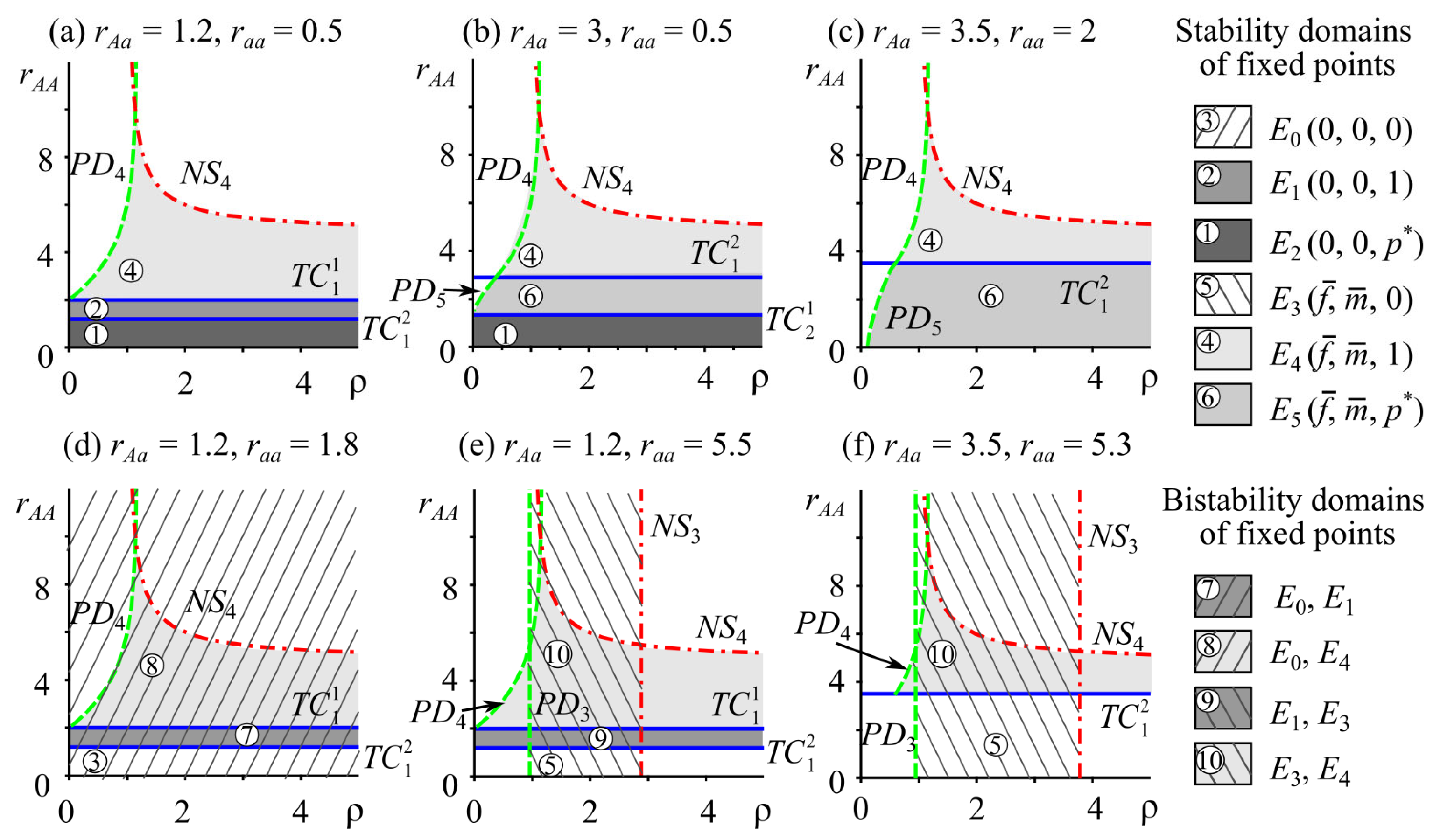
Figure 1. Stability domains of monomorphic and polymorphic fixed points of model (2) with δ = 0.5 in the plane ( ρ , r A A ) . TC, NS, and PD are lines of transcritical, Neimark–Sacker, and period doubling bifurcations, respectively (Table 1).
Mathematics 11 04971 g001
Figure 2. Stability domains of monomorphic and polymorphic fixed points of system (2) with δ = 0.5 , ρ = 1.5 . TC, NS, and PD are lines of transcritical, Neimark–Sacker, and period doubling bifurcations, respectively (Table 1).
Mathematics 11 04971 g002
Figure 3. Trajectories of system (2) at δ = 0.5 , ρ = 1.5 . (a,b) f 0 = 0.2 ,     m 0 = 0.15 , p 0 = 0.1 , (c) f 0 = 0.1 ,     m 0 = 0.14 , p 0 = 0.99998 , (d) f 0 = 0.1 ,     m 0 = 0.12 , p 0 = 6.6 × 10 5 .
Mathematics 11 04971 g003
Figure 4. Trajectories of system (2) at δ = 0.5 , ρ = 1.5 with variation of initial condition. (a) f 0 = 0.3 ,     m 0 = 0.15 , p 0 = 0.5 , (b) f 0 = 0.1 ,     m 0 = 0.1 , p 0 = 0.4 , (c) f 0 = 0.3 ,     m 0 = 0.15 , p 0 = 0.5 , (d) f 0 = 0.1 ,     m 0 = 0.1 , p 0 = 0.6 .
Mathematics 11 04971 g004
Figure 5. Phase portrait (a) and examples of system (2) dynamics with different values of initial conditions (be). The blue and green circles in the phase portrait of system (2) correspond to stable (E4 and E0) and unstable (E1 and E2) fixed points, respectively. B1B4 are the initial points. Arrows indicate the direction of the trajectory. Planes p A = 0 , p A = p * , and p A = 1 define the areas of attraction for fixed points. Vertical dotted lines separate ranges that correspond to neighborhoods of stable (E4 and E0) and unstable (E1 and E2) fixed points.
Mathematics 11 04971 g005
Figure 6. Phase portrait (a) and examples of dynamics for system (2) with different initial conditions (be). The blue and green circles in the phase portrait of system (2) correspond to stable (E3 and E1) and unstable (E0 and E2) fixed points, respectively. B1B4 are the initial points. Arrows indicate the direction of the trajectory. Planes p A = 0 , p A = p * , and p A = 1 define the areas of attraction planes for fixed points. Vertical dotted lines separate ranges that correspond to neighborhoods of stable (E3 and E1) and unstable (E0 and E2) fixed points.
Mathematics 11 04971 g006
Figure 7. Phase portrait (a) and examples of dynamics for system (2) with different initial conditions (be). The blue and green circles in the phase portrait of system (2) correspond to stable (E4 and E3) and unstable (E5) fixed points, respectively. B1B4 are the initial points. Arrows indicate the direction of the trajectory. Planes p A = 0 , p A = p * , and p A = 1 define the areas of attraction planes for fixed points. Vertical dotted lines separate ranges that correspond to neighborhoods of stable (E4 and E3) and unstable (E5) fixed points.
Mathematics 11 04971 g007
Figure 8. Dynamics of allele frequencies p A i , average reproductive potential r ¯ , and group sizes of females f and males m at δ = 0.5 , ρ = 1.5 , and initial conditions f 0 = 0.1 ,     m 0 = 0.1 with (a) p A 0 ( 0 ) = p A 1 ( 200 ) = p A 2 ( 450 ) = p A 3 ( 700 ) = 0.01 , (b) p A 0 ( 0 ) = p A 1 ( 100 ) = p A 2 ( 200 ) = p A 3 ( 350 ) = 0.01 .
Mathematics 11 04971 g008
Table 1. The boundaries of the stability domains of the fixed points of model (2).
Fixed PointsThe Boundaries of Stability Domains
Transcritical bifurcation line (TC)
E0, E3 T C 0 1 : r a a δ 1 = 0 ; T C 0 2 : r a a r A a = 0
E1, E4 T C 1 1 : r A A δ 1 = 0 ; T C 1 2 : r A A r A a = 0
E2, E5 T C 1 2 : r A A r A a = 0 ; T C 0 2 : r a a r A a = 0 ; T C 2 1 : δ ( r A A r a a r A a 2 ) ( r A A 2 r A a + r a a ) = 0
Period doubling bifurcation line (PD)Neimark–Sacker bifurcation line (NS)
E3 P D 3 : ρ = ( δ 1 ) ( r a a δ + 3 ) ( r a a δ 1 ) δ ( r a a 2 δ 2 ( r a a 2 2 r a a ) δ r a a 3 ) N S 3 : ρ = ( δ 1 ) ( r a a δ 1 ) 2 δ ( r a a 2 δ 2 ( r a a 2 + 2 r a a ) δ + 2 r a a + 1 )
E4 P D 4 : ρ = ( δ 1 ) ( r A A δ + 3 ) ( r A A δ 1 ) δ ( r A A 2 δ 2 ( r A A 2 2 r A A ) δ r A A 3 ) N S 4 : ρ = ( δ 1 ) ( r A A δ 1 ) 2 δ ( r A A 2 δ 2 ( r A A 2 + 2 r A A ) δ + 2 r A A + 1 )
E5 P D 5 : ρ = ( B δ + 3 C ) ( δ 1 ) ( B δ C ) δ ( B 2 δ 2 ( B 2 C ) B δ ( B + 3 C ) C ) ,
B = r A A r a a r A a 2 , C = r A A 2 r A a + r a a
N S 5 : ρ = ( δ 1 ) ( B δ C ) 2 δ ( B 2 δ 2 ( B + 2 C ) B δ + ( 2 B + C ) C ) ,
B = r A A r a a r A a 2 , C = r A A 2 r A a + r a a
TC, NS, and PD are lines of transcritical, Neimark–Sacker, and period doubling bifurcations, respectively. The lines of transcritical bifurcations for the following pairs of fixed points E0 and E3, E1 and E4, and E2 and E5 coincide. Subscripts 3–5 in lines NS and PD indicate the number of fixed points (E3E5) that lose their stability.
Disclaimer/Publisher’s Note: The statements, opinions and data contained in all publications are solely those of the individual author(s) and contributor(s) and not of MDPI and/or the editor(s). MDPI and/or the editor(s) disclaim responsibility for any injury to people or property resulting from any ideas, methods, instructions or products referred to in the content.