A Continuous-Time Urn Model for a System of Activated Particles

Abstract

We study a system of M particles with jump dynamics on a network of N sites. The particles can exist in two states, active or inactive. Only the former can jump. The state of each particle depends on its position. A given particle is inactive when it is at a given site, and active when it moves to a change site. Indeed, each sleeping particle activates at a rate $\lambda >0$, leaves its initial site, and moves for an exponential random time of parameter $\mu >0$ before uniformly landing at a site and immediately returning to sleep. The behavior of each particle is independent of that of the others. These dynamics conserve the total number of particles; there is no limit on the number of particles at a given site. This system can be represented by a continuous-time Pólya urn with M balls where the colors are the sites, with an additional color to account for particles on the move at a given time t. First, using this Pólya interpretation for fixed M and N, we obtain the average number of particles at each site over time and, therefore, those on the move due to mass conservation. Secondly, we consider a large system in which the number of particles M and the number of sites N grow at the same rate, so that the $M/N$ ratio tends to a scaling constant $\alpha >0$. Using the moment-generating function technique added to some probabilistic arguments, we obtain the long-term distribution of the number of particles at each site.

1. Introduction

Consider a system of M particles moving among N sites according to a Markovian dynamic. The particles are of two types: active or inactive, according to their positions. Indeed, a given particle $k\in \{1,\dots ,M\}$ in a given site $i\in \{1,\dots ,N\}$ is inactive during an exponential random time of parameter $\lambda$. At the end of this inactivity, the particle k becomes activated and moves to a uniformly chosen site $j\in \{1,\dots ,N\}$. Only activated particles can move among the N sites. See Figure 1. The time for a particle to change site requires a random time whose distribution is exponential with parameter $\mu$. This random time can be seen as movement time due to geographical distance, for example. In this case, parameter $\mu$ represents the inverse of an average site switching time. The total number of particles remains unchanged and there is no limitation on particles per site. Our system is completely homogenous: the model parameters are neither particle- nor site-dependent. The activation of a particle may depend on an external parameter such as a chemical agent or the arrival of an external element. Sleep mode can be seen as a way of saving the energy required for the system to reorganize itself. In this way, particles are only activated to change places. Only this movement generates energy consumption.

Figure 1. M particles moving between N sites. Particles in blue are inactive and those in red are active. The move time of an active particle between two sites, i and j, is random ∼$\mathcal{E}\left(\mu \right)$. The sleep time of an inactive particle ∼$\mathcal{E}\left(\lambda \right)$.

We find this notion of active particles in other contexts, such as interacting random walks, like the frog model, introduced by Durrett. See [1] for more details. A nice application of such models involves the problem of randomized information dissemination in networks for rumor-spread modeling [2]. Indeed, each active particle possesses information that it shares with a particle in standby mode when the former jumps to the latter. The random movement of the particles possessing the information enables it to spread. Also, this system is often taken as a model for the spread of an epidemic over a population [3].

For our model, we are interested in the number of particles on each site at a given time t, denoted by the vector ${\left(X_i\left(t\right)\right)}_{\{1\le i\le N\}}$. Note that due to the mass conservation, the number of particles on the move at time t is given by $X_0\left(t\right)=M-{\sum }_{1\le i\le N}{X}_i\left(t\right)$.

1.1. Physical Motivation

The model of activated particles is a mathematical model used in probability theory to describe the evolution of a system of particles that undergo activation processes. This model is often employed in the study of stochastic processes and can be motivated by various physical phenomena. Here is a general overview of the physical motivation for this problem:

—

Activated particle systems:

• Chemical reactions: A chemical reaction where particles change into an active state and start new reactions could be described by the model.
• Biological systems: This model can be used to simulate biological system activation processes, such as the activation of enzymes or signaling pathways.

—

Stochastic behavior:

• Random activation events: Particle activation is a stochastic process that is impacted by random events in many physical systems. Randomness can be incorporated into the modeling of activation processes using the continuous-time urn model.
• Noise in physical systems: The model might be used to study how noise or fluctuations in a physical system can impact the activation and deactivation of particles.

—

Statistical physics:

• Phase transitions: The model can be connected to the study of phase transitions in statistical physics, where particles undergo a sudden change in behavior or state.
• Thermodynamic equilibrium: Understanding how systems of activated particles reach equilibrium states and the associated thermodynamics.

1.2. Examples

Self-organization is the creation of order from local interactions. It can be observed in many fields of science like physics, chemistry, and biology. For example, in a biological context, an actual issue is the emergence of coherent structures in suspensions of motile particles or microorganisms, like swimming bacteria, such as Escherichia coli or Bacillus subtilis. See [4] for more details. We can also consider a population of cells where individual cells undergo an activation process, such as the activation of immune cells in response to a pathogen. The activated particle system described here is a basic example where the self-organization of the system involves an activation process and mobility between sites.

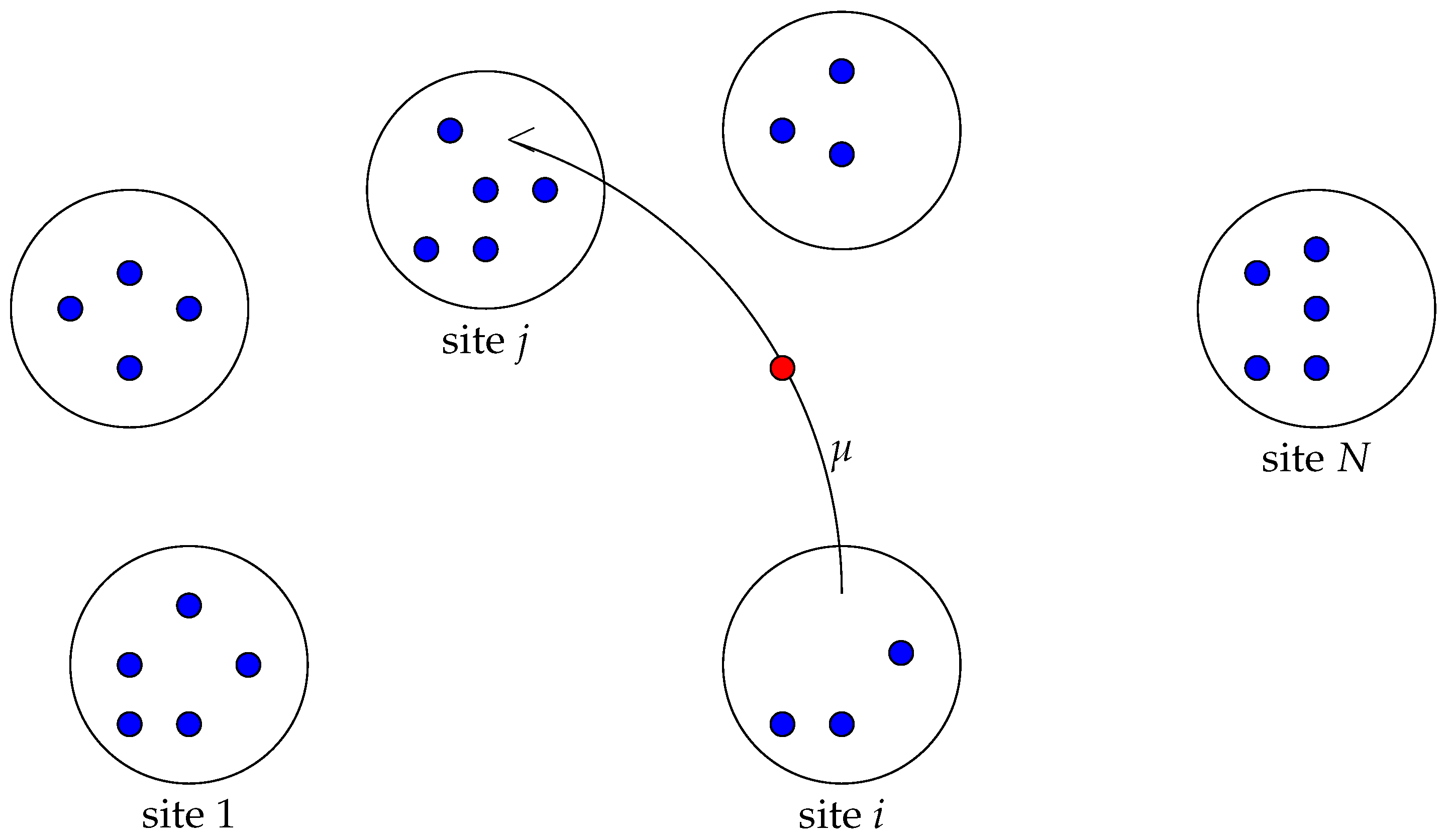
1.3. Continuous-Time Pólya Interpretation

This system can be represented by a continuous-time Pólya urn with M balls where the colors are the sites, with an additional color to account for particles on the move at a given time t. Thus, the number of colors is $N+1$. For $i\in \{0,\dots ,N\}$, $X_i\left(t\right)$ represents the number of balls of color i at time t. Starting from a configuration $(X_0\left(0\right),\dots ,X_N\left(0\right))$, each ball has its own clock, which rings at random time intervals according to an exponential distribution. Each ball’s clock of color $i\in \{1,\dots ,N\}$ follows an exponential distribution of parameter $\lambda$ (the activation of particles in the sites). The balls of color 0 (moving particles) each have a clock following an exponential distribution of parameter $\mu$. The fact that its clock rings implies that the ball in question is picked up and that a ball of color $j\in \{0,\dots ,N\}$ has been added to the urn. Two cases can be distinguished:

–

Activation of a particle on standby at a given site: this concerns a ball of color $i\in \{1,\dots ,N\}$, which will inevitably be replaced by a ball of color 0.

–

Standby mode of a particle initially on the move: this concerns a ball of color 0 which will necessarily be replaced by a ball of color j chosen at random from among colors $1,\dots ,N$.

Thus, let us consider a random variable P having uniform distribution on the set $\left\{1,\cdots ,N\right\}$, and, for all $i\in \left\{1,\cdots ,N\right\}$, let $P_i={\mathbb{I}}_{\{P=i\}}$. Note that ${\sum }_{i=1}^N{P}_i=1$, almost surely. The replacement matrix associated with this continuous-time Pólya urn is random and is given by:

$$\left[\begin{array}{ccccc}-1& P_1& P_2& \cdots & P_N\\ 1& -1& 0& \cdots & 0\\ 1& 0& -1& \cdots & 0\\ ⋮& ⋮& ⋮& ⋮& ⋮\\ 1& 0& \cdots & 0& -1\end{array}\right]$$

This matrix is a generalization of the well-known Ehrenfest urn model [5] (where $N=1$). In our case, we have $(N+1)$ colors, numbered from 0 to N, of balls. Every random time, we remove the drawn ball. If this drawn ball is of color 0, we add uniformly one ball from other colors (from 1 to N), and if the drawn ball is of color $i\ne 0$ we add a ball of color 0.

This urn perfectly models our problem. Overall, the physical motivation for using the continuous-time urn model lies in its ability to capture the stochastic and dynamic nature of systems involving activated particles, providing insights into the underlying processes and behaviors. To our knowledge, this urn has never been studied in the literature except in the case where $N=1$ known as the Ehrenfest urn.

1.4. Related Works

Our model has similarities with the one studied in [6], where the authors are interested in a two-color Pólya urn model whose balls are picked up at random time intervals according to an exponential of parameter 1. They analyze the Ehrenfest process obtained by embedding the discrete evolution in real time. Under tenability conditions, they investigated the associated differential equations for the urn model process to establish an asymptotic solution and prove a distribution convergence to a binomial law.

Contrary to [6], in our model, two types of balls are considered: those of color 0 (particles on the move, i.e., active) and those of other colors (particles on standby in the different sites). This implies that the continuous-time embedding is not done according to the same law: we keep exponential laws but with two different parameters ($\mu$ and $\lambda$) to take into account these two states: active and standby.

The notion of active particles is present in other contexts such as interacting random walks. A simple case, called frog model by Durrett in 1996, can be described as follows: There are active and sleeping particles living on some graphs. Each active particle performs a simple random walk with discrete time and at each moment it may disappear with some probability. When an active particle hits a sleeping particle, the latter becomes active. See [1] for a review of some frog models and results up to 2003. For the frog models, some properties are investigated in the literature like recurrence and transience. See [7,8] for example. Moreover, ref. [9] provides sufficient conditions for the validity of the zero–one law between recurrence and transience of general frog models.

1.5. Outline

This paper is organized as follows. In Section 1, we describe our model, the equivalent continuous-time urn model, and its associated ball addition matrix. We discuss the work related to our model, on two axes: random walks with activated particles on the one hand, and the urns process on the other. Section 2 is dedicated to the average analysis. Section 3 is the main contribution of this work. Indeed, we establish the stationary behavior of the system for fixed N and, therefore, for N, large and obtain a product form. In Section 4, we discuss the model presented here and suggest a heterogeneous variant. We conclude in Section 5 with a possible model of a bike-sharing system as an urn process in an ongoing work. Our main results are Propositions 1 and 2 and Theorems 1 and 2.

2. Average Analysis

We consider the equivalent continuous-time urn model process described as follows: M balls, $(N+1)$ colors denoted by $\{0,\dots ,N\}$. For $i\in \{0,\dots ,N\}$, let $X_i\left(t\right)$ be the number of balls of color i at time t. Starting from an initial configuration $(X_0\left(0\right),\dots ,X_N\left(0\right))$, each ball has its own clock, which rings at random time intervals according to an exponential distribution. The balls of color 0, called type 0 or active, each have a clock following an exponential distribution of parameter $\mu$. Each ball’s clock of color $i\in \{1,\dots ,N\}$ follows an exponential distribution of parameter $\lambda$. These balls are called type 1, or inactive. When its clock rings, the ball in question, say of color i, is picked up and it is replaced by

–

A ball of color 0 if $i\in \{1,\dots ,N\}$;

–

ball of color j chosen at random among colors $1,\dots ,N$ if $i=0$.

Thus, let us consider a random variable P having uniform distribution on the set $\left\{1,\cdots ,N\right\}$, and for all $i\in \left\{1,\cdots ,N\right\}$, let $P_i={\mathbb{I}}_{\{P=i\}}$. Note that ${\sum }_{i=1}^N{P}_i=1$, almost surely. The replacement matrix associated with this continuous-time urn model process is random and is given by the following:

$$\left[\begin{array}{ccccc}-1& P_1& P_2& \cdots & P_N\\ 1& -1& 0& \cdots & 0\\ 1& 0& -1& \cdots & 0\\ ⋮& ⋮& ⋮& ⋮& ⋮\\ 1& 0& \cdots & 0& -1\end{array}\right]$$

The vector of repartition of the balls $\left(X\left(t\right)\right)=(X_0\left(t\right),\dots ,X_N\left(t\right))$ is a Markov process on a finite space

$${\mathcal{S}}_{M,N}=\left\{(k_0,\dots ,k_N)\in {\mathbb{N}}^{N+1},\sum _{i=0}^N{k}_i=M\right\}$$

Let us focus on the number of the balls of color 0 denoted by $\left(X_0\left(t\right)\right)$. The evolution of the process $\left(X_0\left(t\right)\right)$ is as follows:

$$\begin{array}{c}\hfill X_0\left(t+dt\right)=X_0\left(t\right)-\sum _{k=1}^{X_0\left(t\right)}{\mathbb{I}}_{\{d_k^0\le t+dt|d_k^0\ge t\}}+\sum _{i=1}^N\sum _{k_i=1}^{X_i\left(t\right)}{\mathbb{I}}_{\{d_{k_i}^1\le t+dt|d_{k_i}^1\ge t\}}+O\left({\left(dt\right)}^2\right).\end{array}$$

(1)

where for each ball k type $l\in \{0,1\}$, we denote by $d_k^l$ the time at which his clock strikes. This implies, for a type 0 ball, or an active particle on the move, the time when it goes back to sleep, or equivalently the instant when the active particle arrives at its destination site. Thus, $d^0$ follows an exponential law with parameter $\mu$, and vice versa for a type 1 ball, representing a sleeping particle at a given site, it wakes up after an exponential time $d^1$ with parameter $\lambda$.

Due to the exponential lack of memory property, we obtain that, given that the ball’s clock has not rung until the instant t, the probability that it will run before the instant $t+dt$ is the same as the probability that a clock reset to zero will run before the instant $dt$.

In a similar way to active particles, we can write the evolution equation for the process $\left(X_i\left(t\right)\right)$ of the number of inactive particles at a given site $1\le i\le N$, as follows:

$$\begin{array}{c}\hfill X_i(t+dt)=X_i\left(t\right)-\sum _{k_i=1}^{X_i\left(t\right)}{\mathbb{I}}_{\{d_k^1\le t+dt|d_k^1\ge t\}}+{\delta }_i\sum _{k=1}^{X_0\left(t\right)}{\mathbb{I}}_{\{d_k^0\le t+dt|d_k^0\ge t\}}+O\left({\left(dt\right)}^2\right)\end{array}$$

(2)

where ${\delta }_i={\mathbb{I}}_{\left\{\mathrm{site} i \mathrm{is} \mathrm{uniformly} \mathrm{chosen} \mathrm{as} \mathrm{destination}\right\}}$. For $1\le i\le N$, the random variable ${\delta }_j$ has a Bernoulli distribution with parameter $1/N$.

2.1. Active Particles or Balls of Type 0

Let $m_0\left(t\right)=\mathbb{E}\left[X_0\left(t\right)\right]$ denote the average number of balls of color 0 at time $t\ge 0$. Suppose that all the particles are inactive (distributed on the N sites) in the initial configuration and then $m_0\left(0\right)=0$, we obtain the explicit expression of $m_0\left(t\right)$.

Proposition 1.

For $t\ge 0$, one obtains

$$m_0\left(t\right)=\frac{\lambda M}{\mu +\lambda }\left(1-\exp \left(-(\mu +\lambda )t\right)\right).$$

and

$$\underset{t\to +\infty }{\lim }{m}_0\left(t\right)=\frac{\lambda M}{\mu +\lambda }.$$

Proof. 

By the conditional expectation on the evolution Equation (1), we obtain

$$m_0\left(t+dt\right)=m_0\left(t\right)-m_0\left(t\right)\left(1-e^{-\mu dt}\right)+\sum _{i=1}^N{m}_i\left(t\right)\left(1-e^{-\lambda dt}\right)+O\left({\left(dt\right)}^2\right).$$

When $dt$ goes to zero, we obtain

$$m_0^{\prime }\left(t\right)=-\mu m_0\left(t\right)+\lambda \sum _{i=1}^N{m}_i\left(t\right).$$

(3)

Due to the mass conservation, it holds that ${\sum }_{i=1}^N{m}_i\left(t\right)=M-m_0\left(t\right)$. We deduce

$$m_0^{\prime }\left(t\right)=-\left(\mu +\lambda \right)m_0\left(t\right)+\lambda M.$$

Since in the initial configuration all the particles are inactive, then $m_0\left(0\right)=0$. We simply solve this differential equation to obtain the explicit expression of $m_0\left(t\right)$ for $t\ge 0$. The limit is immediate. □

Remark 1.

–

Note that the average number of balls of color 0 does not depend on the parameter N. Indeed, for balls of color 0 (active particles), the other colors do not differ in terms of behavior and are, therefore, not distinguishable.

–

When $N=1$ (two colors) and $\lambda =\mu =1$, we obtain a model that is very close to the one studied in [6], but is less general since the replacement matrix in [6] is given by

$$\left[\begin{array}{cc}-\alpha & \beta \\ \alpha & -\beta \end{array}\right]$$

with positive integers α and β, when in our case a drawn ball is replaced by another ball of a different color ($\alpha =\beta =1$).

–

For the trivial case $M=N=1$ (one ball, two colors), we obtain for all $t>0$:

$$\begin{array}{c}\hfill X_0\left(t\right)has as distribution\mathrm{Ber}\left(\frac{\lambda }{\lambda +\mu }\left(1-e^{(\lambda +\mu )}\right)\right)\end{array}$$

2.2. Inactive Particles or Balls of Type 1

For $i\in \{1,\dots ,N\}$, let $m_i\left(t\right)=\mathbb{E}\left[X_i\left(t\right)\right]$ be the average number of balls of color i at time $t\ge 0$. Suppose that all the particles are inactive and uniformly distributed on the N sites in the initial configuration and then $m_i\left(0\right)=M/N$. we obtain the explicit expression of $m_0\left(t\right)$. In a similar way to active particles, we obtain the following result:

Proposition 2.

For $i\in \{1,\dots ,N\}$ and $t\ge 0$, one obtains

$$m_i\left(t\right)=\frac{M}{N}\frac{\lambda \mu }{\mu +\lambda }\left(\frac{1}{\lambda }+\frac{e^{-(\mu +\lambda )t}}{\mu }\right).$$

and then

$$\underset{t\to +\infty }{\lim }{m}_i\left(t\right)=\frac{M}{N}\frac{\mu }{\mu +\lambda }.$$

Proof. 

By the conditional expectation on the evolution Equation (2), we obtain

$$m_i(t+dt)=m_i\left(t\right)-m_i\left(t\right)\left(1-e^{-\lambda dt}\right)+m_0\left(t\right)\left(1-e^{-\mu dt}\right)\frac{1}{N}+O\left({\left(dt\right)}^2\right),$$

When $dt$ goes to zero, we obtain

$$m_i^{\prime }\left(t\right)=-\lambda m_i\left(t\right)+m_0\left(t\right)\frac{\mu }{N}.$$

(4)

Since all the particles are inactive and uniformly distributed on the N sites in the initial configuration and then $m_i\left(0\right)=M/N$, replacing $m_0\left(t\right)$ by its expression, we conclude. □

3. Distribution Analysis

In this section, we investigate the distribution of both the number of active and inactive particles.

3.1. Active Particles or Balls of Type 0

We investigate the distribution of the number of active particles, or equivalently, the number of balls of color 0, at time $t\ge 0$, using the moment-generating function method. The MGF approach is widely used in similar cases. For all $t\ge 0$, for all $u=\left(u_0,\cdots ,u_N\right)\in {\mathbb{R}}^{N+1}$, we define $\varphi$ the moment-generating function of the vector $X\left(t\right)=\left(X_0\left(t\right),\cdots ,X_N\left(t\right)\right)$ by

$$\varphi \left(t,u\right)=\mathbb{E}\left[\exp \left(⟨u,X\left(t\right)⟩\right)\right]=\mathbb{E}\left[\exp \left(\sum _{i=0}^N{u}_i{X}_i\left(t\right)\right)\right].$$

For $v:=u_0$, denote by $\Psi (v,t):=\varphi \left(t,(v,0,\cdots ,0)\right)$. First, let us start with a technical lemma.

Lemma 1.

For $v\mathbb{R}$ and $t\ge$, the following differential equation of the function Ψ holds:

$$\frac{\partial }{\partial t}\Psi \left(t,v\right)=\left[\lambda \left(1-e^v\right)-\mu \left(1-e^{-v}\right)\right]\frac{\partial }{\partial v}\Psi \left(t,v\right)-\lambda M\left(1-e^v\right)\Psi \left(t,v)\right),$$

(5)

with the initial condition $\Psi \left(0,v)\right)=\Psi \left(t,0)\right)=1$.

Proof. 

For $v\in \mathbb{R}$ and $t\ge 0$, denote by $\Psi (v,t):=\varphi \left(t,(v,0,\cdots ,0)\right)$. Then, using the evolution Equation (1), we obtain

$$\begin{array}{ccc}\hfill \Psi \left(t+dt,v\right)& =& \mathbb{E}\left[\exp \left(v{X}_0(t+dt)\right)\right]\hfill \\ & =& \mathbb{E}\left[\exp \left(v{X}_0\left(t\right)-v\sum _{k=1}^{X_0\left(t\right)}{\mathbb{I}}_{\{d_k^0\left(t\right)\le dt\}}+v\sum _{i=1}^N\sum _{k_i=1}^{X_i\left(t\right)}{\mathbb{I}}_{\{d_{k_i}^1\left(t\right)\le dt\}}+O\left({\left(dt\right)}^2\right)\right)\right]\hfill \\ & =& \mathbb{E}\left[\mathbb{E}\left\{\exp \left(v{X}_0\left(t\right)-v\sum _{k=1}^{X_0\left(t\right)}{\mathbb{I}}_{\{d_k^0\left(t\right)\le dt\}}+v\sum _{i=1}^N\sum _{k_i=1}^{X_i\left(t\right)}{\mathbb{I}}_{\{d_{k_i}^1\left(t\right)\le dt\}}+O\left({\left(dt\right)}^2\right)\right)|X_0\left(t\right)\right\}\right]\hfill \\ & =& \mathbb{E}\left[e^{v{X}_0\left(t\right)}\mathbb{E}\left\{\exp \left(-v\sum _{k=1}^{X_0\left(t\right)}{\mathbb{I}}_{\{d_k^0\left(t\right)\le dt\}}+v\sum _{i=1}^N\sum _{k_i=1}^{X_i\left(t\right)}{\mathbb{I}}_{\{d_{k_i}^1\left(t\right)\le dt\}}+O\left({\left(dt\right)}^2\right)\right)|X_0\left(t\right)\right\}\right]\hfill \\ & =& \mathbb{E}\left[e^{v{X}_0\left(t\right)}{\left[\mathbb{E}\left(e^{-v{\mathbb{I}}_{\{d_k^0\left(t\right)\le dt\}}}\right)\right]}^{X_0\left(t\right)}{\left[\mathbb{E}\left(e^{v{\mathbb{I}}_{\{d_k^1\left(t\right)\le dt\}}}\right)\right]}^{{\sum }_{i=1}^N{X}_i\left(t\right)}\left(1+O_p\left(d{t}^2\right)\right)\right]\hfill \\ & =& \mathbb{E}\left[e^{v{X}_0\left(t\right)}{\left[\mathbb{E}\left(e^{-v{\mathbb{I}}_{\{d_k^0\left(t\right)\le dt\}}}\right)\right]}^{X_0\left(t\right)}{\left[\mathbb{E}\left(e^{v{\mathbb{I}}_{\{d_k^1\left(t\right)\le dt\}}}\right)\right]}^{M-X_0\left(t\right)}\left(1+O_p\left(d{t}^2\right)\right)\right]\hfill \\ & =& \mathbb{E}\left[e^{v{X}_0\left(t\right)}{[e^{-v}\left(1-e^{-\mu dt}\right)+e^{-\mu dt}]}^{X_0\left(t\right)}{[e^v\left(1-e^{-\lambda dt}\right)+e^{-\lambda dt}]}^{M-X_0\left(t\right)}\left(1+O_p\left(d{t}^2\right)\right)\right]\hfill \\ & =& \mathbb{E}\left[e^{v{X}_0\left(t\right)}{e}^{\left(-\mu X_0\left(t\right)\left(1-e^{-v}\right)dt\right)}{e}^{\left(-\lambda \left(M-X_0\left(t\right)\right)\left(1-e^v\right)dt\right)}\left(1+O_p\left(d{t}^2\right)\right)\right]\hfill \\ & =& \mathbb{E}\left[e^{v{X}_0\left(t\right)}{e}^{-\left[\mu \left(1-e^{-v}\right)-\lambda \left(1-e^v\right)\right]X_0\left(t\right)dt}\left(1+O_p\left(d{t}^2\right)\right)\right]e^{-\lambda M\left(1-e^v\right)dt}\hfill \\ & =& \mathbb{E}\left[e^{v{X}_0\left(t\right)}\left(1+\left(\lambda \left(1-e^v\right)-\mu \left(1-e^{-v}\right)\right)X_0\left(t\right)dt\right)\left(1+O_p\left(d{t}^2\right)\right)\right]e^{-\lambda M\left(1-e^v\right)dt}.\hfill \end{array}$$

Then, one obtains

$$\Psi \left(t+dt,v\right)-\Psi \left(t,v\right)=\left(\lambda \left(1-e^v\right)-\mu \left(1-e^{-v}\right)\right)\mathbb{E}\left[e^{X_0\left(t\right)v}{X}_0\left(t\right)\right]dt-\lambda M\left(1-e^v\right)\mathbb{E}\left[e^{X_0\left(t\right)v}\right]dt+O_p\left(d{t}^2\right).$$

When $dt$ goes to zero, we obtain the above differential equation. □

The next step is the resolution of the differential Equation (5), which is the key argument for establishing the following distribution convergence.

Theorem 1

(Distribution convergence). For all $t\ge 0$, one obtains

$$X_0\left(t\right)\stackrel{D}{\underset{t\to +\infty }{⟶}}\mathrm{Bin}\left(M,\frac{\lambda }{\mu +\lambda }\right)$$

a binomial distribution with parameters $\left(M,\frac{\lambda }{\mu +\lambda }\right)$.

Proof. 

For all $t\ge 0$ and $v\in \mathbb{R}$, since $X_0\left(t\right)\in \left\{0,\cdots ,M\right\}$, one obtains that

$$\Psi \left(t,v\right)=\sum _{k=0}^M{e}^{vk}\mathbb{P}\left(X_0\left(t\right)=k\right).$$

The differential Equation (5) established in Lemma 1 can be written as follows:

$$\begin{array}{ccc}\hfill \sum _{k=0}^M{e}^{vk}\frac{\partial }{\partial t}\mathbb{P}\left(X_0\left(t\right)=k\right)& =& \left[\lambda \left(1-e^v\right)-\mu \left(1-e^{-v}\right)\right]\sum _{k=0}^{M}k{e}^{vk}\mathbb{P}\left(X_0\left(t\right)=k\right)\hfill \\ & -& \lambda M\left(1-e^v\right)\sum _{k=0}^M{e}^{vk}\mathbb{P}\left(X_0\left(t\right)=k\right).\hfill \\ \\ & =& \left(\lambda -\mu \right)\sum _{k=0}^{M}k{e}^{vk}\mathbb{P}\left(X_0\left(t\right)=k\right)-\lambda \sum _{k=1}^{M}k{e}^{v(k+1)}\mathbb{P}\left(X_0\left(t\right)=k\right)\hfill \\ & +& \mu \sum _{k=1}^{M}k{e}^{v(k-1)}\mathbb{P}\left(X_0\left(t\right)=k\right)-\lambda M\sum _{k=0}^M{e}^{vk}\mathbb{P}\left(X_0\left(t\right)=k\right)\hfill \\ & +& \lambda M\sum _{k=0}^M{e}^{v(k+1)}\mathbb{P}\left(X_0\left(t\right)=k\right).\hfill \end{array}$$

By the change of variable, we obtain

$$\begin{array}{ccc}\hfill \sum _{k=0}^M{e}^{vk}\frac{\partial }{\partial t}\mathbb{P}\left(X_0\left(t\right)=k\right)& =& \left(\lambda -\mu \right)\sum _{k=0}^{M}k{e}^{vk}\mathbb{P}\left(X_0\left(t\right)=k\right)-\lambda \sum _{k=1}^{M+1}(k-1)e^{vk}\mathbb{P}\left(X_0\left(t\right)=k-1\right)\hfill \\ & +& \mu \sum _{k=0}^{M-1}(k+1)e^{vk}\mathbb{P}\left(X_0\left(t\right)=k+1\right)-\lambda M\sum _{k=0}^M{e}^{vk}\mathbb{P}\left(X_0\left(t\right)=k\right)\hfill \\ & +& \lambda M\sum _{k=1}^{M+1}{e}^{vk}\mathbb{P}\left(X_0\left(t\right)=k-1\right)\hfill \end{array}$$

which implies, after simplification

$$\begin{array}{ccc}\hfill \sum _{k=0}^M{e}^{vk}\frac{\partial }{\partial t}\mathbb{P}\left(X_0\left(t\right)=k\right)& =& \left(\lambda -\mu \right)\sum _{k=0}^{M}k{e}^{vk}\mathbb{P}\left(X_0\left(t\right)=k\right)-\lambda \sum _{k=1}^M(k-1)e^{vk}\mathbb{P}\left(X_0\left(t\right)=k-1\right)\hfill \\ & +& \mu \sum _{k=0}^{M-1}(k+1)e^{vk}\mathbb{P}\left(X_0\left(t\right)=k+1\right)-\lambda M\sum _{k=0}^M{e}^{vk}\mathbb{P}\left(X_0\left(t\right)=k\right)\hfill \\ & +& \lambda M\sum _{k=1}^{M+1}{e}^{vk}\mathbb{P}\left(X_0\left(t\right)=k-1\right).\hfill \end{array}$$

To deal with this differential equation, we introduce the following matrix notation, for $t\ge 0$ and $k\in \{0,\dots ,M\}$:

$$\begin{array}{ccc}\hfill P_{(0,k)}\left(t\right)& =& \mathbb{P}\left(X_0\left(t\right)=k\right)\hfill \\ \hfill P_0\left(t\right)& =& \left[\begin{array}{c}{P}_{(0,0)}\left(t\right)\\ P_{(0,1)}\left(t\right)\\ P_{(0,2)}\left(t\right)\\ ⋮\\ P_{(0,M)}\left(t\right)\end{array}\right],\mathrm{with}\sum _{k=0}^M{P}_{(0,k)}\left(t\right)=1.\hfill \end{array}$$

From the last equation, and since Equation (5) is true for all v, we deduce that, for all $k\in \{1,\dots ,M-1\}$, one obtains the following:

$$\begin{array}{ccc}\hfill \frac{\partial }{\partial t}{P}_{(0,k)}\left(t\right)& =& \lambda \left[M-k+1\right]P_{(0,k-1)}\left(t\right)+\left[\left(\lambda -\mu \right)k-\lambda M\right]P_{(0,k)}\left(t\right)+\mu \left(k+1\right)P_{(0,k+1)}\left(t\right),\hfill \\ \hfill \frac{\partial }{\partial t}{P}_{(0,0)}\left(t\right)& =& \mu P_{(0,1)}\left(t\right)-\lambda M{P}_{(0,0)}\left(t\right),\hfill \\ \hfill \frac{\partial }{\partial t}{P}_{(0,M)}\left(t\right)& =& \lambda P_{(0,M-1)}\left(t\right)-\mu M{P}_{(0,M)}\left(t\right).\hfill \end{array}$$

We define A as the square matrix of order $(M+1)$ by

$$A=\left[\begin{array}{ccccc}-\lambda M& \mu & 0& \cdots & 0\\ \lambda M& \lambda -\mu -\lambda M& 2\mu & 0\cdots 0& 0\\ ⋮& ⋮& ⋮& ⋮& ⋮\\ 0& \cdots 0& 2\lambda & -\mu \left(M-1\right)-\lambda & M\mu \\ 0& \cdots & 0& \lambda & -\mu M\end{array}\right].$$

Then the vector $P_0\left(t\right)$ satisfies the following differential equation:

$$\frac{\partial }{\partial t}{P}_0\left(t\right)=A{P}_0\left(t\right),$$

(6)

with the initial condition

$$P_0\left(0\right)=\left[\begin{array}{c}1\\ 0\\ 0\\ ⋮\\ 0\end{array}\right].$$

We, thus, find the same differential equation treated in [6] with the same matrix A. According to [6], the solution of the Equation (6) is given by

$$P_0\left(t\right)=e^{At}{P}_0\left(0\right)=T\left[\begin{array}{ccccc}1& 0& 0& \cdots & 0\\ 0& e^{-(\lambda +\mu )}& & 0\cdots 0& 0\\ ⋮& ⋮& ⋮& ⋮& ⋮\\ 0& \cdots 0& 0& e^{-(M-1)(\lambda +\mu )}& 0\\ 0& \cdots & 0& 0& e^{-M(\lambda +\mu )}\end{array}\right]T^{-1}{P}_0\left(0\right),$$

where T is the associated transition matrix. We recognize here that Matrix A is a member of a Leonard pair of the Krawtchouk type, where the eigenvalues are all simple and form an arithmetic progression. Then there exists some positive constant a and a constant ${\lambda }_0$, such that the eigenvalues of A are:

$${\lambda }_0,{\lambda }_0-a,{\lambda }_0-2a,\cdots ,{\lambda }_0-Ma.$$

Since the sum of all eigenvalues of a matrix must be equal to its trace, we deduce that

$$a=\frac{2{\lambda }_0}{M}+\mu +\lambda .$$

Then using [6], we deduce the desired result. □

Remark 2.

This method does not seem to allow us to obtain a similar result concerning the distribution of the number of inactive particles at a given site $i\in \{1,\dots ,N\}$ at a fixed time $t\ge 0$. Indeed, the joint distribution $(X_0\left(t\right),X_i\left(t\right))$ is necessary. The MGF approach used to obtain the exact distribution of $X_0\left(t\right)$ results in a differential equation whose explicit solution is far more complicated.

3.2. Inactive Particles or Balls of Type 1

The vector of repartition of the inactive particles on the N sites $\left(X\left(t\right)\right)=(X_1\left(t\right),\dots ,X_N\left(t\right))$ is a Markov process on the finite space

$${\tilde{\mathcal{S}}}_{M,N}=\left\{(k_1,\dots ,k_N)\in {\mathbb{N}}^N,\sum _{i=0}^N{k}_i\le M\right\}.$$

Moreover, it is irreducible and, thus, it admits a stationary distribution, denoted by $(X_1(\infty ),\dots ,X_N(\infty ))$. The following result explicitly establishes the long-time repartition of the inactive particles on the N sites.

Theorem 2.

The stationary distribution $(X_1(\infty ),\dots ,X_N(\infty ))$ has a product form, such that for $i\in \{1,\dots ,N\}$, and the random variable $X_i(\infty )$ has a binomial distribution, $\mathrm{Bin}\left(M,\frac{\mu }{N\left(\mu +\lambda \right)}\right)$.

Proof. 

Recall that due to the homogeneity of the system, for fixed $t\ge 0$, all $\left(X_i\left(t\right)\right)$ have the same distribution for $i=1,\dots ,N$. Moreover, given that there are $k\in \{0,\cdots ,M\}$ inactive particles, which is equivalent to $(M-k)$ active particles on the move, the distribution of the vector $\left(X_1\left(t\right),\cdots ,X_N\left(t\right)\right)$ follows a multinomial distribution with parameter k and $\left(1/N,\cdots ,1/N\right)$. Thus, for all $\left(k_1,\cdots ,k_N\right)$, such that ${\sum }_{i=1}^N{k}_i=k\le M$, we obtain the following:

$$\begin{array}{ccc}\hfill \mathbb{P}\left(X_1\left(t\right)=k_1,\cdots ,X_N\left(t\right)=k_N\right)& =& \mathbb{P}\left(X_1\left(t\right)=k_1,\cdots ,X_N\left(t\right)=k_N,X_0\left(t\right)=M-k\right)\hfill \\ \\ & =& \mathbb{P}\left(X_1\left(t\right)=k_1,\cdots ,X_N\left(t\right)=k_N/X_0\left(t\right)=M-k\right)\mathbb{P}\left(X_0\left(t\right)=M-k\right)\hfill \\ \\ & =& \frac{k!}{k_1!\cdots k_N!}{N}^{-k}\mathbb{P}\left(X_0\left(t\right)=M-k\right).\hfill \end{array}$$

It is sufficient to use the explicit expression for the distribution of $X_0\left(t\right)$ set out in Section 3. Thus, one has

$$\begin{array}{ccc}\hfill \underset{t\to +\infty }{\lim }\mathbb{P}\left(X_1\left(t\right)=k_1,\cdots ,X_N\left(t\right)=k_N\right)& =& \frac{k!}{k_1!\cdots k_N!}{N}^{-k}\underset{t\to +\infty }{\lim }\mathbb{P}\left(X_0\left(t\right)=M-k\right)\hfill \\ & =& \frac{k!}{k_1!\cdots k_N!}{N}^{-k}{\left(\frac{\lambda }{\mu +\lambda }\right)}^{M-k}{\left(\frac{\mu }{\mu +\lambda }\right)}^k\left(\genfrac{}{}{0pt}{}{M}{M-k}\right)\hfill \\ & =& \left(k!\prod _{i=1}^N{\left(\frac{\mu }{N(\mu +\lambda )}\right)}^{k_i}\frac{1}{k_i!}\right)\left({\left(\frac{\lambda }{\mu +\lambda }\right)}^{M-k}\frac{M!}{k!(M-k)!}\right)\hfill \\ & =& \left(\left(\genfrac{}{}{0pt}{}{k}{k_1,\cdots ,k_N}\right)\prod _{i=1}^N{\left(\frac{\mu }{N(\mu +\lambda )}\right)}^{k_i}\right)\left(\left(\genfrac{}{}{0pt}{}{M}{M-k}\right){\left(\frac{\lambda }{\mu +\lambda }\right)}^{M-k}\right)\hfill \\ & =& eM!\hfill \\ & & \times \prod _{i=1}^N\exp \left(-\frac{\mu }{N(\mu +\lambda )}\right){\left(\frac{\mu }{N(\mu +\lambda )}\right)}^{k_i}\frac{1}{k_i!}\hfill \\ & & \times \exp \left(-\frac{\lambda }{\mu +\lambda }\right){\left(\frac{\lambda }{\mu +\lambda }\right)}^{M-k}\frac{1}{(M-k)!}\hfill \\ & =& M!{\left(\frac{\lambda }{\mu +\lambda }\right)}^{M-k}\frac{1}{(M-k)!}\prod _{i=1}^N{\left(\frac{\mu }{N(\mu +\lambda )}\right)}^{k_i}\frac{1}{k_i!}\hfill \end{array}$$

which is the desired result. □

Remark 3.

The vector $(X_1,\cdots ,X_N)$ depends on both the time t and system size N (number of sites). We chose to simplify the notations by omitting the index N. However, this choice should not lead us to forget the dependence on N of the stationary distribution, which will be noted as follows:

$$(X_1^N(\infty ),\dots ,X_N^N(\infty )).$$

The product form for the stationary distribution of the vector $(X_1\left(t\right),\cdots ,X_N\left(t\right))$ holds under the constraint that ${\sum }_{i=1}^N{X}_1^N(\infty )\le M$.

As our focus is on large particle systems (N large), and since in our case, the total number of particles M is proportional to the number of sites N, such that ${\lim }_{N\to +\infty }M/N=\alpha >0$, using Theorem 2 and a classical result of convergence of binomial distribution to Poisson distribution, we obtain the following result:

Proposition 3.

If ${\lim }_{N\to +\infty }M/N=\alpha >0$, then one obtains

$$\begin{array}{ccc}\hfill X_i(\infty )& & \stackrel{D}{\underset{N\to +\infty }{⟶}}\mathrm{Poi}\left(\frac{\alpha \mu }{\mu +\lambda }\right),i=1,\cdots ,N,\hfill \\ \\ \hfill \frac{\mu +\lambda }{\sqrt{\mu \lambda }}\frac{X_0(\infty )-\frac{M/\lambda }{\mu +\lambda }}{\sqrt{M}}& & \stackrel{D}{\underset{N\to +\infty }{⟶}}\mathcal{N}\left(0,1\right).\hfill \end{array}$$

Remark 4.

When N becomes large (and, therefore, M, since $M/N\sim \alpha$ for N large), the constraint of mass conservation does not hold anymore. For a finite number of components ${\left(X_i(\infty )\right)}_{i\ge 1}$, these random variables are i.i.d.

4. Discussion

The model studied in this article is a homogeneous model in which the standby and activation parameters are not site-dependent. When a particle is moving, the choice of a site as the destination is uniform. The advantage of such a model is its natural formulation as a continuous-time Pólya urn. We can consider a slightly more general model by introducing spatial heterogeneity: a particle in sleep mode at a given site i wakes up with a rate ${\lambda }_i$ and moves to a given site j with a rate ${\mu }_{\{⇝j\}}$. Let us introduce the average vector $M\left(t\right)$ defined by:

$$M\left(t\right)=\left[\begin{array}{c}{m}_0\left(t\right)\\ m_1\left(t\right)\\ m_2\left(t\right)\\ ⋮\\ m_{N-1}\left(t\right)\end{array}\right].$$

Recall that $m_n\left(t\right)=M-{\sum }_{k=0}^{N-1}{m}_k\left(t\right)$. Equations (3) and (4) are written in this case as:

$$\begin{array}{cc}\hfill m_0^{\prime }\left(t\right)=& -\overline{\mu }{m}_0\left(t\right)+\sum _{k=1}^N{\lambda }_k{m}_k\left(t\right)\hfill \\ \hfill m_i^{\prime }\left(t\right)=& \frac{{\mu }_{\{⇝i\}}}{N}{m}_0\left(t\right)-{\lambda }_i{m}_i\left(t\right),\mathrm{for}\mathrm{all}i=1,\cdots ,N\hfill \end{array}$$

where

$$\overline{\mu }=\frac{1}{N}\sum _{k=1}^N{\mu }_{\{⇝k\}}.$$

We deduce that the vector $M\left(t\right)$ can be easily obtained by resolution of the following differential equation

$$M^{\prime }\left(t\right)=\left[\begin{array}{ccccc}-\left(\overline{\mu }+{\lambda }_N\right)& {\lambda }_1-{\lambda }_N& {\lambda }_2-{\lambda }_N& \cdots & {\lambda }_{N-1}-{\lambda }_N\\ N^{-1}{\mu }_{\{⇝1\}}& -{\lambda }_1& & 0\cdots 0& 0\\ ⋮& ⋮& ⋮& ⋮& ⋮\\ N^{-1}{\mu }_{\{⇝N-2\}}& \cdots 0& 0& -{\lambda }_{N-2}& 0\\ N^{-1}{\mu }_{\{⇝N-1\}}& \cdots & 0& 0& -{\lambda }_{N-1}\end{array}\right]M\left(t\right)+{\lambda }_{N}M\left[\begin{array}{c}1\\ 0\\ 0\\ ⋮\\ 0\end{array}\right].$$

The study of the system’s distribution is more complicated. Indeed, the Pólya urn approach used in this paper is not suited to heterogeneity, as the continuous embedding does not lend itself to it. We state a result relating to the asymptotic distribution of the system in a weaker case when independent of the site ${\lambda }_i=\lambda$. In this case, for $t\ge 0$, one obtains

$$m_0\left(t\right)=\frac{\lambda M}{\lambda +\overline{\mu }}\left(1-\exp \left(-\left(\overline{\mu }+\lambda \right)t\right)\right).$$

and

$$\underset{t\to +\infty }{\lim }{m}_0\left(t\right)=\frac{\lambda M}{\lambda +\overline{\mu }}.$$

For all $i=1,\cdots ,N:$

$$m_i\left(t\right)=\frac{M}{N}\frac{\lambda {\mu }_{\{⇝i\}}}{{\mu }_{\{⇝i\}}+\lambda }\left(\frac{1}{\lambda }+\frac{e^{-({\mu }_{\{⇝i\}}+\lambda )t}}{{\mu }_{\{⇝i\}}}\right).$$

and then

$$\underset{t\to +\infty }{\lim }{m}_i\left(t\right)=\frac{M}{N}\frac{{\mu }_{\{⇝i\}}}{{\mu }_{\{⇝i\}}+\lambda }.$$

The same result holds for the distributions, we just have to replace $\mu$

• By $\overline{\mu }=\frac{1}{N}{\sum }_{i=1}^N{\mu }_{\{⇝i\}}$ in the asymptotic distribution of $\left(X_0\left(t\right)\right)$;
• By ${\mu }_{\{⇝i\}}$ in the asymptotic distribution of $\left(X_i\left(t\right)\right)$.

5. Conclusions

In this article, we explore a model of particles moving between N sites, switching between inactive and active states. The system is homogeneous, characterized by site-independent parameters. Our investigation focuses on the asymptotic behavior of a system composed of M particles distributed over the N sites, where M and N grow at the same rate. Although the model considered is simple, the novelty of this work is the formulation as a continuous-time Pólya urn when the number of colors and balls tend toward infinity at the same rate. Naturally, the next step of this work is to investigate a completely heterogeneous model in which the movement of a given particle between two sites i and j follows an exponential distribution with parameter ${\mu }_{\{i⇝j\}}$ and the wake-up time of a given particle on standby at a site i follows an exponential distribution with parameter ${\lambda }_i$. A different approach is required to address heterogeneity, as the continuous-time Pólya urn model is not appropriate A more general framework involves making all these parameters dependent on both the site and the particle. This approach effectively abandons the assumption that, in the equivalent urn model process, the particles are no longer indistinguishable. It should be noted that, due to the homogeneity of the parameters, the problem being considered can be transformed into the study of a Markov chain with two states: active or inactive. However, this approach is not suitable for the heterogeneous case and is not the focus of this work.

A different version of this model, where sites switch from inactive to active (instead of particles), leads to a situation where an active site “wakes up” one of its particles, if it has any at that moment, to send it to a site chosen uniformly among the N sites. This models a bike-sharing system. The sites are the stations and the particles are the bikes. See [10] for a mean-field analysis of a homogenous model and [11,12] for an inhomogeneous model. This kind of system does not translate naturally into an urn model process, as it is not the balls that “ring”, but rather the colors. This model is part of ongoing work to develop an urn model equivalent to a bike-sharing system.

References

- Popov, S.Y. Frogs and some other interacting random walks models. In Proceedings of the Discrete Mathematics & Theoretical Computer Science, 4th International Conference, DMTCS 2003, Dijon, France, 7–12 July 2003. [Google Scholar]
- Giakkoupis, G.; Mallmann-Trenn, F.; Saribekyan, H. How to spread a rumor: Call your neighbors or take a walk? In Proceedings of the 2019 ACM Symposium on Principles of Distributed Computing, Toronto, ON, Canada, 29 July–2 August 2019; pp. 24–33. [Google Scholar]
- Benjamini, I.; Fontes, L.R.; Hermon, J.; Machado, F.P. On an epidemic model on finite graphs. Ann. Appl. Probab. 2020, 30, 208–258. [Google Scholar] [CrossRef]
- Saintillan, D.; Shelley, M.J. Emergence of coherent structures and large-scale flows in motile suspensions. J. R. Soc. Interface 2012, 9, 571–585. [Google Scholar] [CrossRef] [PubMed]
- Ehrenfest, P.; Ehrenfest, T. Über zwei bekannte Einwände gegen das Boltzmannsche H-Theorem. Physik 1907, 8, 311–314. [Google Scholar]
- Balaji, S.; Mahmoud, H.M.; Watanabe, O. Distributions in the Ehrenfest process. Stat. Probab. Lett. 2006, 76, 666–674. [Google Scholar] [CrossRef]
- Hoffman, C.; Johnson, T.; Junge, M. From transience to recurrence with Poisson tree frogs. Ann. Appl. Probab. 2016, 26, 1620–1635. [Google Scholar] [CrossRef]
- Hoffman, C.; Johnson, T.; Junge, M. Recurrence and transience for the frog model on trees. Ann. Probab. 2017, 45, 2826–2854. [Google Scholar] [CrossRef]
- Kosygina, E.; Zerner, M.P. A zero-one law for recurrence and transience of frog processes. Probab. Theory Relat. Fields 2017, 168, 317–346. [Google Scholar] [CrossRef]
- Fricker, C.; Gast, N. Incentives and redistribution in homogeneous bike-sharing systems with stations of finite capacity. EURO J. Transp. Logist. 2016, 5, 261–291. [Google Scholar] [CrossRef]
- Fricker, C.; Tibi, D. Equivalence of ensembles for large vehicle-sharing models. Ann. Appl. Probab. 2017, 27, 883–916. [Google Scholar] [CrossRef]
- Fricker, C.; Gast, N.; Mohamed, H. Mean field analysis for inhomogeneous bike sharing systems. In Proceedings of the 23rd International Meeting on Probabilistic, Combinatorial, and Asymptotic Methods for the Analysis of Algorithms (AofA’12), Montreal, QC, Canada, 1 January 2012. [Google Scholar]
Disclaimer/Publisher’s Note: The statements, opinions and data contained in all publications are solely those of the individual author(s) and contributor(s) and not of MDPI and/or the editor(s). MDPI and/or the editor(s) disclaim responsibility for any injury to people or property resulting from any ideas, methods, instructions or products referred to in the content. |
© 2023 by the authors. Licensee MDPI, Basel, Switzerland. This article is an open access article distributed under the terms and conditions of the Creative Commons Attribution (CC BY) license (https://creativecommons.org/licenses/by/4.0/).