Abstract
The choice of the factorization rank of a matrix is critical, e.g., in dimensionality reduction, filtering, clustering, deconvolution, etc., because selecting a rank that is too high amounts to adjusting the noise, while selecting a rank that is too low results in the oversimplification of the signal. Numerous methods for selecting the factorization rank of a non-negative matrix have been proposed. One of them is the cophenetic correlation coefficient (), widely used in data science to evaluate the number of clusters in a hierarchical clustering. In previous work, it was shown that performs better than other methods for rank selection in non-negative matrix factorization (NMF) when the underlying structure of the matrix consists of orthogonal clusters. In this article, we show that using the ratio of to the approximation error significantly improves the accuracy of the rank selection. We also propose a new criterion, , which, like , benefits from the stochastic nature of NMF; its accuracy is also improved by using its ratio-to-error form. Using real and simulated data, we show that , with a CUSUM-based automatic detection algorithm for its original or ratio-to-error forms, significantly outperforms . It is important to note that the new criterion works for a broader class of matrices, where the underlying clusters are not assumed to be orthogonal.
Keywords:
clustering; dimensionality reduction; machine learning; NMF; cophenetic correlation coefficient; concordance; CUSUM MSC:
65F55; 62H30
1. Introduction
Non-negative matrix factorization (NMF) [1,2] is a linear dimensionality reduction technique that has become popular for its ability to automatically extract sparse and easily interpretable factors [3], detect similarity between subsets of patients sharing local patterns of gene expression data [4], cluster the rows or columns of a matrix [5], perform filtering and deconvolution tasks [6,7], and interpret social phenomena through topic modeling [8], to name just a few applications.
Let be a non-negative matrix. For a given rank c such that , a non-negative factorization of M is given by:
with: , , , .
The non-negative matrices and are called the components of the factorization, and the tensor product above is the regular product between and the transpose of . We use the tensor product notation because it symmetrizes the respective roles of W and H, and also because it is easily generalized to the context of tensor factorization. In order to simplify the notation, in what follows we drop the indices denoting the matrix size when there is no ambiguity. Each row of M can be seen as a single observation of f different features or attributes, stored in f distinct columns of M. Equation (1) allows us to express the observations in M in a more parsimonious way by reducing the original number f of features to a smaller number c. The tradeoff for this simplified representation is the presence of the factorization error term represented by matrix E.
Let us refer to the c synthetic features whose values populate the rows of matrix W as “meta-features”. The transition from the condensed representation in the space of meta-features to the “physical” representation is provided by the matrix H, which plays the role of a transition matrix. A single observation from M is represented by its ith row , and each column of H, say k, yields the decomposition of as a non-negative linear combination of c meta-features , with being the column of H, such that the following relation holds:
Non-negative matrix factorization has a geometric interpretation that makes it easier to understand: up to a certain approximation error coded in the matrix E, each observation vector belongs to the non-negative simplex generated by the c vectors. Non-negative matrix factorization can also be seen as a projection on this simplex, with the distance from the matrix to the simplex being the approximation error . If we add null columns to W and H and obtain and with the same number of rows and c’> c columns, the tensor product of these matrices remains unchanged: , hence . It follows that when the factorization rank increases, the approximation error is non-increasing. As an immediate consequence, an exact factorization at rank c remains exact at any larger rank . If one was only dealing with exact factorizations, the optimal factorization rank could be defined as the lowest rank for which the factorization is exact. Unfortunately, the additional noise makes the situation more complicated: there is no obvious information to extract from the non-increasing series of approximation errors . Therefore, an important question is whether the selected rank leads to a “meaningful” decomposition, since choosing a rank that is too high amounts to adjusting the noise, while choosing a rank that is too low leads to oversimplification of the signal.
In [9], several methods were evaluated, e.g., Velicer’s Minimum Average Partial, Minka’s Laplace–PCA, Bayesian Information Criterion (BIC), and Brunet’s cophenetic correlation coefficient () [10]. Another method is the minimum description length approach that selects the rank that ensures the best possible encoding of the data [11]. For this approach, the encoding also covers the noise, so a low signal-to-noise ratio tends to inflate the effects of the noise. Cross-validation can also be used to select the rank that provides the most accurate imputation of missing data [12]. Depending on the method used, significantly different ranks may be selected [13]. Of course, in principle, using the results of all available methods together should help with the selection of the proper rank. Unfortunately, simple heuristic rules to do that have not been found yet, which led to the idea of using deep learning approaches.
In [14], the starting idea was that several metrics may be potentially useful for rank selection. The authors included the approximation error as well as penalized versions like the AIC or BIC criteria. NMF clustering stability metrics, such as the silhouette coefficient, were also included. Because none of these metrics can indicate on their own which rank should be selected by simply observing the values taken for different ranks (a graph referred to as a scree-plot), the authors have entrusted a neural network, taking some candidate metrics as inputs, with the task of determining a (non-linear) function of the metrics that can be used to select the correct rank. Because this network has to work well for many types of matrices, it needs to be trained on a large and diverse set of matrices. These matrices are constructed such that their rank is known, and this rank is used as a label in the training set. The network presented by the authors worked well for matrices of the same type as those from the training set, but it did not perform well when applied to different types of matrices. The lack of generalizability to non-synthetic matrices is due to the inherent limitation of using a simulation framework, which, even if well designed, it is not able to reproduce all types of matrices that may be encountered in real life. Nevertheless, it is of interest to determine which specific metrics or combinations of metrics are most useful for selecting the correct factorization rank for synthetic datasets, even if each individual metric is not sufficient on its own. Unfortunately, the results from [14] do not provide any insights with regard to this.
The estimates of the NMF components are inherently stochastic [15]: the NMF estimates are obtained through iterative updating rules that offer no guarantee of converging to a global minimum, making them sensitive to initial “guessed” values. Yang et al. [16] propose to alleviate this problem by mutually complementing NMF and Deep Learning. However, their approach is essentially based on a multilayer NMF, first proposed in [17], and far beyond the scope of this work, which is focused on a single-layer NMF. By contrast, the cophenetic correlation coefficient, , fully exploits the stochastic nature of the NMF estimates without requiring any training: for a given factorization rank, provides an estimate of the consistency of the co-clustering of observations or features that can be derived from the NMF components over multiple runs of the algorithm, each using a random initialization [10]. The factorization rank is chosen to maximize this consistency. The wide use of in practice, thanks to its availability in common NMF packages [18,19], and its relatively good performance on synthetic matrices with orthogonal underlying factors [9], has led us to use it as a reference metric while introducing a new criterion, which we call . The latter also exploits the stochastic nature of the NMF estimates, this time by examining their stability relative to reference estimates obtained by non-negative double singular value decomposition (NNDSVD) [20] up to some permutation. To evaluate the performance of our new criterion and compare it to the criterion, we apply a CUSUM-based automatic detection algorithm to publicly available datasets and to synthetic matrices. In addition, we show that considering the ratio of or to the approximation error significantly decreases the rank selection error. Remarkably, our new criterion works very well with a broader class of matrices than those tested in [9], namely matrices for which the underlying factors are not assumed to be orthogonal.
2. Materials and Methods
2.1. Public Datasets
In this section we present four publicly available datasets that were used to evaluate the rank selection methods.
2.1.1. Brunet Dataset
Golub et al. [21] report data on the associations between the gene expression of 7129 genes and disease status. There are 11 patients with acute myeloid leukemia (AML) and 27 patients with acute lymphoblastic leukemia (ALL). The ALL group is further divided into T- and B-cell subtypes (19 and 8 patients, respectively). The B-cell subtype group was further divided into two subgroups in [22]. We consider only the 5000 well-expressed genes used by Brunet et al. [10]. Prior to performing NMF, we take the logarithm of the gene expression values and subtract the baseline value, calculated as the minimum expression value for each gene. The resulting data set is called the Brunet data set, and its rank is 4.
2.1.2. Sausage Dataset
Ellekjær et al. [23] ran a designed experiment where three constituents—fat, salt, and starch—added when making sausages, were varied according to a single-replicate 6 × 3 × 3 factorial design. For the 54 sausages analyzed, fat had six levels (8%, 12%, 16%, 20%, 24%, 28%); salt had three levels (1.3%, 1.6%, 1.9%); and starch had three levels (1.5%, 4.5%, 7.5%). The 54 sausages were measured by both sensory analysis and NIR spectroscopy. We analyze only the spectral data. NIR spectra were measured in 4 nm increments from wavelengths ranging from 1100 nm to 2498 nm, and so there are 351 measurements per sausage. Accordingly, the NIR matrix has 54 rows and 351 columns. We refer to this dataset as the Sausage dataset, and its rank is 3.
2.1.3. Swimmer Dataset
Donoho and Stodden [24] created the Swimmer dataset to illustrate conditions for uniqueness of the NMF decomposition. It depicts a figure with a fixed torso and four moving parts (limbs), each able to exhibit four articulations (different positions). Each image contains 12 pixels in the center (for the fixed torso) and four limbs of 6 pixels each that can be in one of four positions. All possible combinations of limb positions give us 256 images. The rank of this dataset is 17.
2.1.4. Mnist Dataset
The MNIST dataset [25] consists of 70,000 hand-written Arabic numerals divided into a 60,000 element training set and a 10,000 element testing set. The MNIST dataset was originally constructed for the training and testing of machine learning algorithms used to classify hand-written digits. The rank of this dataset is 10.
2.2. Artificial Matrices with Prespecified Rank
To construct artificial matrices with prespecified rank, we considered two complementary approaches, which can be summarized as follows:
- The BouquetsFirst approach: W and H are explicitly structured into clusters with specified correlation levels within clusters and between clusters. The rank is equal to the number of clusters. In this approach, the degree of sparsity of the components W and H is a direct consequence of the number of clusters and specified correlation levels.
- The Sparsity First approach: The degrees of sparsity for W and H are explicitly specified. In this approach, the components W and H are structured into clusters that are more or less clearly defined depending on the degree of sparsity and the size of the matrix.
- Mixed approaches, e.g., W (resp. H) is constructed with the bouquets first approach and H (resp. W) is constructed with the sparsity first approach.
A specified amount of noise is then added to the constructed matrix. Expressed in relative terms, the noise is drawn from an uniform distribution on (0, 0.25).
2.2.1. Bouquets First
The idea behind the bouquet method is to construct a matrix whose rows (i.e., observations) are naturally grouped according to the column containing their dominant coefficient. Let us start with a canonical case: each of the n (resp. f) rows of the matrix W (resp. H) are zero everywhere except for one non-zero coordinate among the c dimensions. We can then group the rows according to the single non-zero coefficient. If we construct a matrix W and a matrix H based on this method, the product is a matrix containing c independent blocks, and it is not possible to represent it with fewer than c blocks. Let us start with a W (resp. H) matrix having the following structure:
where the following compatibility relation holds for W (resp. H):
As long as none of the is zero, it is clear that the row vectors of W and H need exactly c dimensions. The matrix M has the following generic structure:
In this canonical case, we see that M is a block matrix, made of c non-overlapping matrices. For such matrices, it is clear that exactly c components allow for their reconstruction, and that their factorization could not be achieved with a smaller rank.
- The principle of the bouquet method is to generalize the previous construction by relaxing the condition of a single non-zero coefficient imposed to the rows of the matrix:
- By replacing the c mutually orthogonal vectors from with c “weakly correlated” vectors from .
- By imposing to each row of the matrix to be “strongly correlated” with exactly one of the previous vectors.
Algorithm 1 builds a set of vector bouquets. Each bouquet comprises a variable number of vectors whose correlation with a given vector, identified as the “centroid” of the bouquet, is higher than a prescribed minimum correlation threshold. The mutual correlations of the centroids have to be less than a prescribed maximum correlation threshold.
| Algorithm 1 Build a set of bouquet vectors |
| Require: , , , |
| Build c centroid vectors in |
| Generate a random partition of [1, nbvec] with c integers: |
| for do |
| Generate vectors correlated with centroid : |
| for do |
| Find small random vector in , orthogonal to such that Correlation(, ) ≥ and in |
| end for |
| end for |
| Return vectors in |
Algorithm 2 returns c random vectors from having a mutual correlation less than . These vectors are obtained by adding to each coordinate vector of a value generated from a uniform distribution on an open interval having 0 as the lower bound and an upper bound depending on the prescribed maximum correlation.
- More precisely, let us use the following notations:
- is the ith coordinate vector of , for .
- , are c random vectors with coordinates independently drawn from the uniform distribution .
- .
- An upper bound on the cosine of the angle between vectors and for is set by imposing the condition: .
Using the expressions of the first two moments of a uniform distribution: , , it is easy to verify that:
- = .
- .
- After substitutions, the upper bound condition stated above yields a quadratic inequality in : .
- Provided that , this equation has a unique positive solution in , representing the maximum allowed magnitude of a uniform perturbation applied to orthogonal unitary vectors, in order to provide an upper bound for their mutual cosine.
| Algorithm 2 Make centroids |
| Require: , |
| Unique positive solution in X of |
| for do |
| coordinate vector of |
| end for |
| Return |
2.2.2. Sparsity First
Here we generate matrices by controlling the sparsity [26] of the W and H components. First, each component is randomly generated. Then, sparsity is enforced at the specified level for each component as described in [27]. Algorithm 3 takes as input a matrix of size and a sparsity level and returns a sparse matrix where, for each column of : . For each column of , there are non-zero values (where depends on the column), which define a cluster. However, since the sparsity enforcement is carried out independently for each component, there is no guarantee that clusters will not overlap between components. Therefore, the sparsity first approach automatically results in clusters that are more or less clearly defined depending on the degree of sparsity and the size of the matrix. We have considered 2 versions of this algorithm, and , where for the first version the sparsity level is randomly selected from a uniform distribution on [0.5, 1], and so its minimum value is 0.5, while for the second version it is randomly selected from a uniform distribution on [0, 0.5], and so its maximum value is 0.5.
| Algorithm 3 Make a sparse matrix |
| Require: , |
| for each column of do |
| Set |
| Normalize: |
| Set |
| Set and |
| Get a mapping such that and for all valid |
| Compute values of as follows: |
| for do |
| if then |
| break |
| end if |
| end for |
| Set and to zero otherwise. |
| Set corresponding column y of : |
| end for |
| Return |
2.2.3. Overview of the Dataset of Artificial Matrices
The non-parametric approach presented in this article is based on optimizing the trade-off between stochastic stability (as measured by concordance) and the approximation error. Given that, a training set of matrices is not necessary. For the purpose of evaluating the performance of rank selection methods, a dataset of 2500 random matrices has been built by reverse-engineering the NMF factorization process. One starts with a (W, H) pair of matrices sharing the same number of columns, equal to the prespecified rank c. A matrix is then generated (a detailed description is given in Algorithm 4). The rank c of the matrix M is used as a benchmark for any rank selection method. The performance of the various methods is statistically evaluated on this set of 2500 random matrices. We will use the term “rank estimation error” to refer to the rank selection error in the context of this statistical evaluation.
2.3. Criteria for Rank Selection
It can be argued that the interpretability of NMF factors comes at a certain price: the lack of a unique solution. This is in contrast to singular value decomposition (SVD), whose factors, on the other hand, are less interpretable due to their mixed signs. A nice example of a simple matrix that can be factorized exactly by two completely distinct sets of non-negative components can be found in [28]. Although conditions for uniqueness of the solution can be found in [24], they can hardly be checked in practice. With respect to the rank selection problem, we will see that this lack of uniqueness is actually a blessing, since it leads to alternative criteria that perform better than the approximation error criterion commonly used for SVD. Specifically, we present two criteria for NMF rank selection that benefit from the stochastic nature of the NMF components: the popular cophenetic correlation coefficient () and a new criterion we call .
| Algorithm 4 Generate a set of random matrices with prespecified rank |
| Require: , |
| /* and are respectively the minimum and maximum ranks of generated matrices, set here to 3 and 27.*/ |
| /* and are respectively the maximum inter-correlation (of bouquets centroids), and minimum intra-correlation (of vectors within a bouquet), set here to 0.2 and 0.8. */ |
| /* is the maximum level of multiplicative noise applied to an exact factorization, set here to 25%. */ |
| /* is the minimum number of rows of a W or H matrix, set here to 10 times the number of components. */ |
| /* is the maximum number of rows of a W or H matrix, set here to 300. */ |
| for do |
| for do |
| ] |
| if == bouquet then |
| else |
| if == min_sparsity then |
| else |
| end if |
| end if |
| if then |
| , |
| else |
| , |
| end if |
| end for |
| /* Entries of matrix N are independently drawn from a normal distribution */ |
| /* A multiplicative noise is applied to the product of components */ |
| end for |
| Return |
2.3.1. Cophenetic Correlation Coefficient
Due to their non-convexity, NMF algorithms may not converge to the same solution depending on the initial conditions. The strategy proposed by Brunet et al. [10] is to run the algorithm several times with different random initial conditions and, for each run, assign the observations to clusters based on the relative values in each column of W. If the selected rank is correct, this assignment is unlikely to change much from run to run, and so the evaluation of its stability is useful to select the correct rank. To this end, a consensus matrix C is computed at each run, where the entry is if observations i and j belong to the same cluster, and if they belong to different clusters. C is then averaged over all runs and is defined as the Pearson correlation of two distance matrices: the first, , is the distance between observations induced by the consensus matrix, and the second is the distance between observations induced by the linkage used in reordering C. The pseudocode is given in Algorithm 5. The same approach can be applied to H, and then the geometric average of the based on W and H can be calculated.
| Algorithm 5 calculation for W |
| Require: |
| for do |
| Run NMF with random initialization |
| Save component estimates in W (random components) |
| Calculate consensus matrix |
| for do |
| if observations i and j belong to the same cluster, else |
| end for |
| end for |
| over all iterations |
2.3.2. Concordance
In contrast to using random initializations, the non-negative double singular value decomposition (NNDSVD) has been shown to lead to a rapid reduction of the approximation error [20]. Taking the NNDSVD estimates as reference, the average distance D between the W estimates obtained with random initialization and the reference estimates is given by , where is calculated with the pseudocode given in Algorithm 6. The same approach can be applied to H, and then the geometric average of based on W and H can be calculated.
| Algorithm 6 calculation for W |
| Require: |
| Run NMF with NNDSVD initialization |
| Save component estimates in (reference components) |
| for do |
| Run NMF with random initialization |
| Save component estimates in W (random components) |
| for do |
| Look for the reference component in maximizing correlation with |
| Save the index of the found component and its correlation with the random component |
| end for |
| over indices |
| Set and |
| end for |
| over all iterations |
Based on Algorithm 6, reaches its maximum value of 1 when each component obtained by random initialization corresponds to a unique reference component with which it is perfectly correlated. If two or more randomly initialized components correspond to the same reference component, or if the correlation is less than 1, then decreases.
To prevent a slight bias in Algorithm 6, the number of unique indices, which normally varies between 1 and c, has been adjusted to vary between 0 and c, using the following transformation: , where x is the number of unique indices.
2.3.3. Ratio of ccc or Concordance to the Approximation Error
To illustrate why considering the ratio of or to the approximation error is beneficial, let us return to the Brunet dataset. Brunet et al. [10] have shown that the hierarchical structure of the leukemia dataset can be retrieved by NMF. With only two clusters, patients with AML are distinguished from patients with ALL. With three clusters, ALL patients are further subdivided into T-cell (ALL-T) and B-cell (ALL-B) subtypes. Finally, with 4 clusters, the ALL-B subtype is further divided into two clusters. Since decreases significantly only when the number of clusters exceeds 4, any of the ranks 2, 3, or 4 may be selected. However, the approximation error decreases rapidly from rank 2 to 4, indicating that factorizing the data with rank 2 or 3 leads to an oversimplification of the underlying biology. However, the ratio of to the approximation error () has a maximum at rank 4.
2.4. Rank Selection
Our strategy is to compute the criterion over a range of possible ranks. Based on the obtained values, a CUSUM chart is created to automatically select the rank, as described in Algorithm 7.
| Algorithm 7 CUSUM chart for rank selection |
|
To summarize Algorithm 7, is incremented by 1 if the criterion is decreasing between ranks c and , otherwise 1 is subtracted from , which cannot be less than 0. In fact, the selected rank corresponds to the beginning of two consecutive decreases of the criterion.
3. Results
3.1. Results on Artificial Matrices
3.1.1. Distribution of the Rank Estimation Error
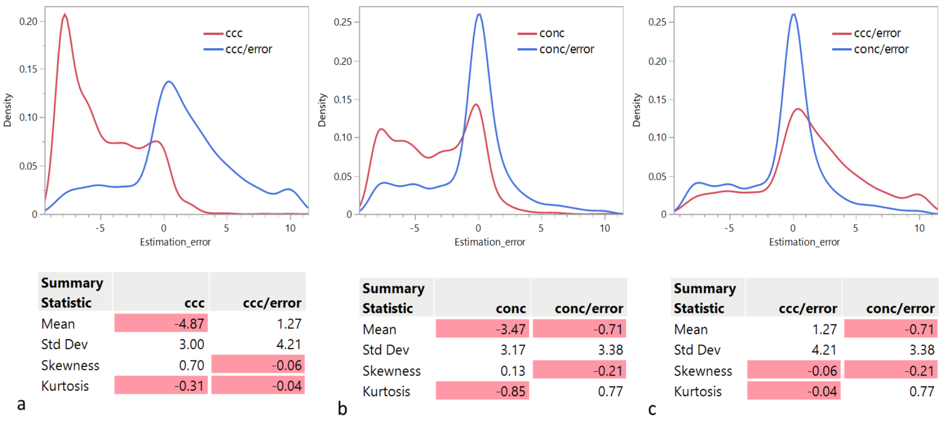
In this section, we examine the distribution of the rank estimation error as a function of the criterion used. The quartiles of the distributions are given in Table 1. Panels a and b in Figure 1 show that the distributions of the rank estimation error using or indicate a strong tendency to underestimate the actual rank. However, is better than in this regard: Median for = −6 and Median for = −3. We observe that both distributions are bimodal, with a second mode around 0 and longer tails to the right, resulting in an overall positive skewness. However, the main mode for is the negative one, while the main mode for is the one around 0. Remarkably, this tendency is significantly reduced when each criterion is divided by the approximation error: Median for = 1 and Median for = 0. Panel c in Figure 1 compares the distributions of the rank estimation error using and , indicating a strong tendency of to overestimate the actual rank: 3rd quartile for = 4, while 3rd quartile for = 1.

Table 1.
Quartiles of the distribution of the rank estimation error as a function of the criterion used.
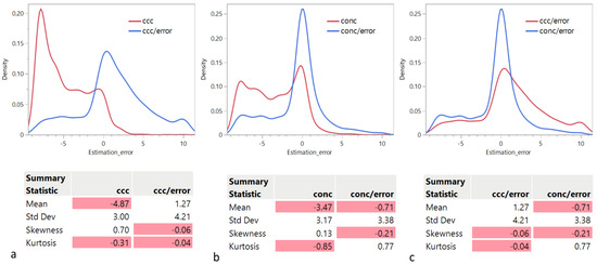
Figure 1.
Distribution of the rank estimation error as a function of the criterion used: (a) vs. , (b) () vs. , and (c) vs. . The negative values are highlighted in red.
3.1.2. Sources of Error
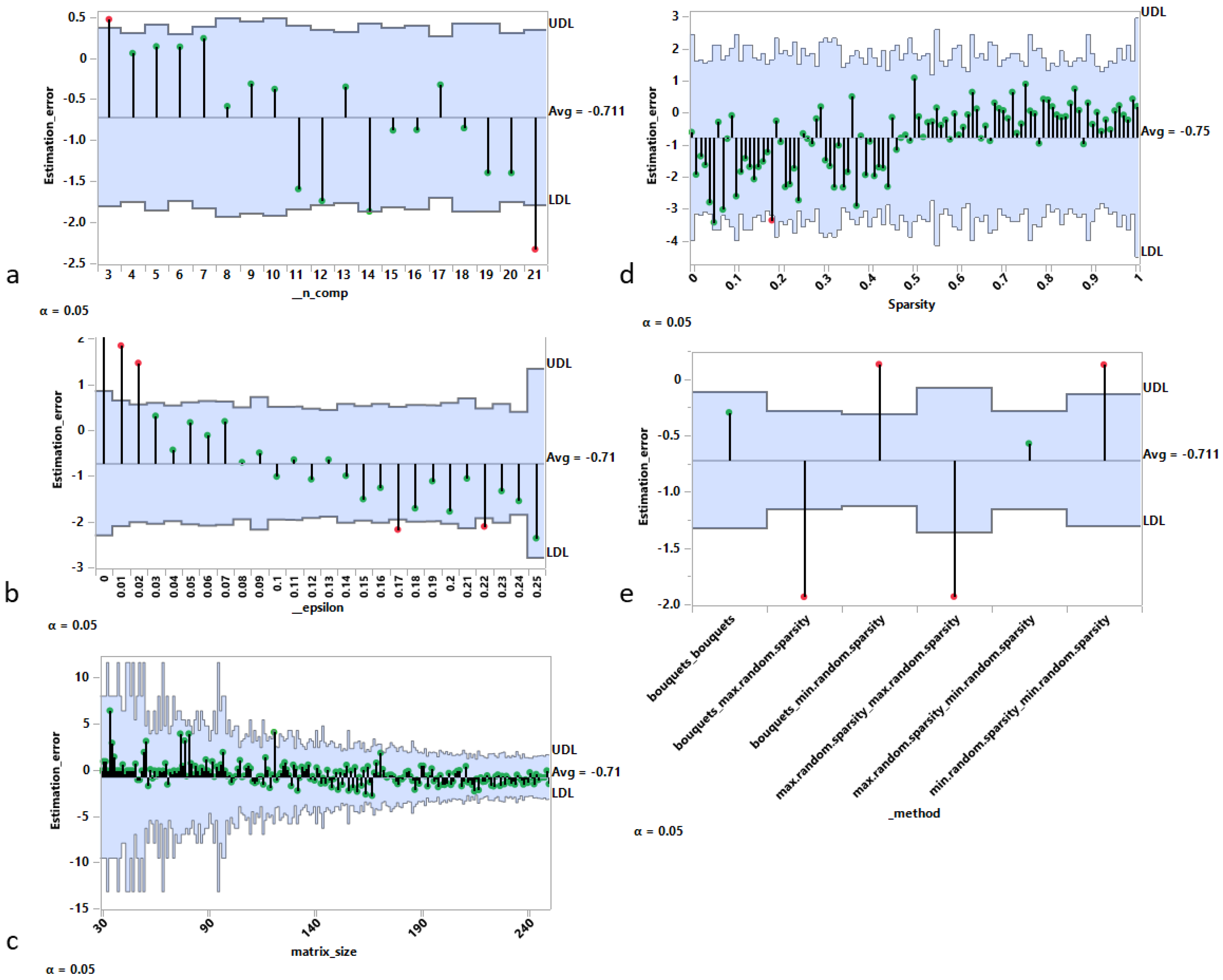
In this section, we examine the main sources of rank estimation error for the best performing criterion, , as shown in the previous Section 3.1.1, using the analysis of mean representation [29]. In Figure 2, each panel contains a decision chart with the following elements:
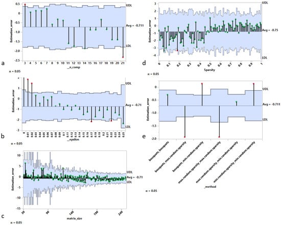
Figure 2.
Sources of rank estimation error using analysis of means (ANOM) approach. Rank estimation error vs. (a) real rank, (b) noise intensity, (c) matrix size (in either dimension), (d) sparsity of underlying components, and (e) algorithms used to generate the artificial matrices.
- An upper decision limit (UDL).
- A lower decision limit (LDL).
- The center line position is determined by the overall mean.
The following empirical observations can be drawn from the charts:
- Panel a shows that the estimation error (estimated rank minus real rank) has an overall decreasing tendency as a function of the real rank (i.e., the number of components used to generate the matrix), with a maximum value for c = 3 and a minimum value for c = 21.
- Panel b also shows an overall decreasing tendency of the rank estimation error as a function of the level of noise used to generate the matrix. In particular, from 15% and above, the real rank is systematically underestimated.
- Panel c indicates a bias for matrices of moderate size (with the size defined as the maximum between the number of rows and the number of columns) resulting in an overall overestimation of the rank.
- Panel d investigates the estimation error as a function of the sparsity level (Algorithm 3) used to generate the matrix. For sparsity levels less than 0.5 (i.e., dense matrices), the rank is on average underestimated, while the opposite is true for sparsity levels above 0.5.
- Panel e shows the average estimation error for each of the six possible generation methods obtained by combining pairwise the bouquets method, the minimum sparsity level method, and the maximum sparsity level method for the generation of the random matrices W and H (Algorithm 4). The results show clearly that:
- −
- Setting a maximum level of sparsity for one component or both results in a significant underestimation bias.
- −
- Setting a minimum level of sparsity for one component or both results in a significant overestimation bias.
The preceding empirical observations lead us to consider two types of matrices. The first type are matrices that have an unambiguous factorization, i.e., linked to a sharp optimum in Equation (1). These matrices are characterized by a low level of noise and a high level of parsimony. The second type are matrices that have a factorization linked to a very flat optimum. These matrices are characterized by a high level of noise and a high density of coefficients. For the first type of matrices, we expect to observe a very clear local maximum on the criterion around the true rank. This peak can be observed before the CUSUM condition (i.e., two consecutive drops after the maximum) is reached, and hence the observed overestimation bias. For the second type of matrices, the high level of noise creates higher fluctuations in the term around the true rank. It also makes the decrease in error less marked as a function of the true rank. There is a significant probability of observing the expected decrease of the before the true rank, and hence the observed underestimation bias.
3.2. Results on Public Datasets
The results obtained with the synthetic matrices have led us to consider the ratio of or to the approximation error, while applying automatic rank selection based on the CUSUM chart.
3.2.1.
For the MNIST dataset, severely underestimates the actual rank of 10 with an estimated rank of 4. The Sausage and Brunet datasets confirm that tends to overestimate the rank, as was the case in our simulations, with estimated ranks of 4 and 5, instead of the true ranks of 3 and 4, respectively. For the Swimmer dataset, the estimated rank of 17 is equal to the actual rank.
3.2.2.
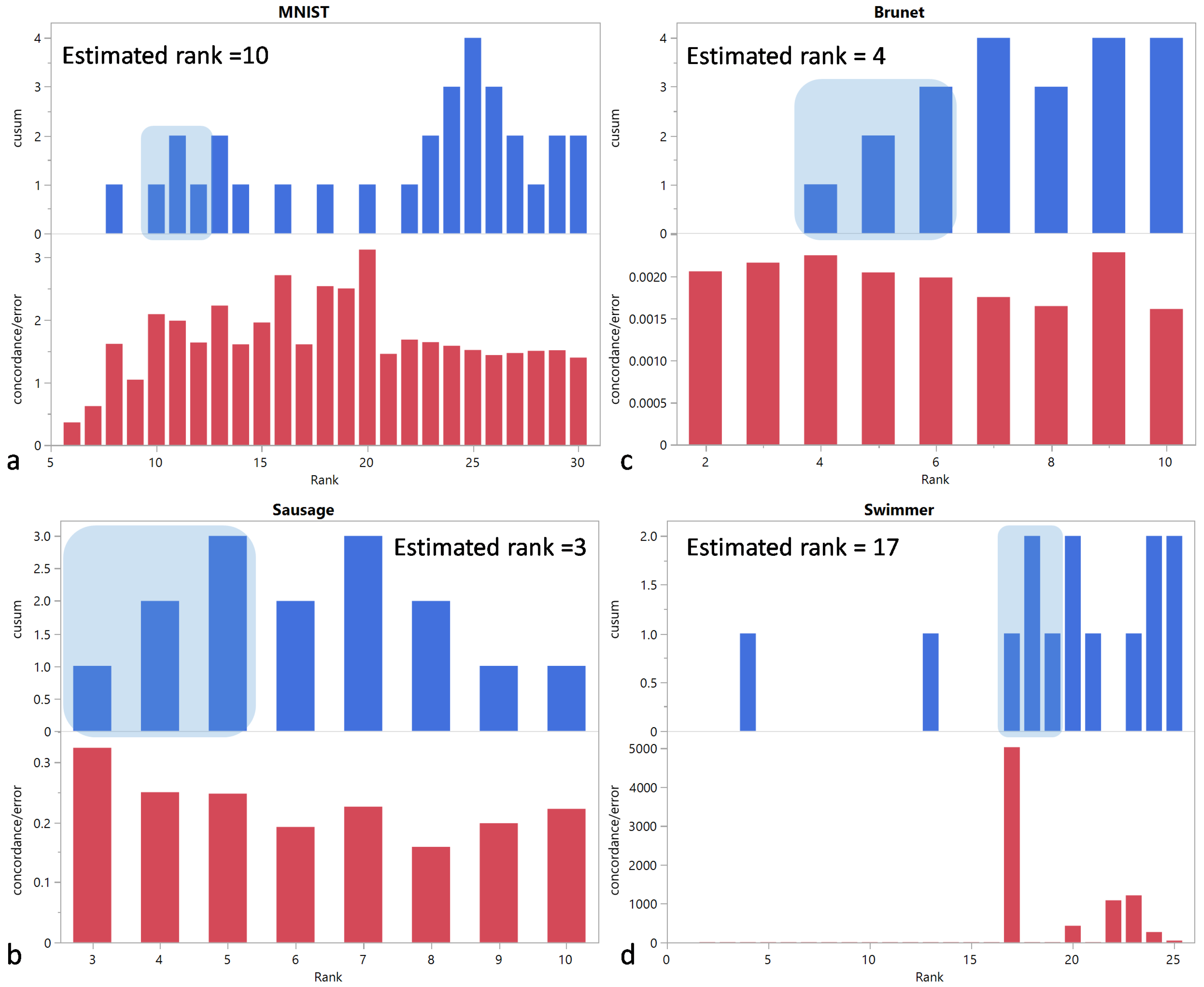
The estimated ranks are 10, 3, 4, and 17 for the MNIST, Sausage, Brunet, and Swimmer datasets, respectively, and they are equal to the actual ranks (Figure 3).
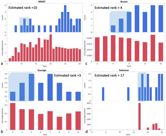
Figure 3.
and vs. rank for (a) MNIST, (b) Sausage, (c) Brunet, and (d) Swimmer datasets. The shaded area corresponds to the first region of the CUSUM chart with three consecutive positive values. The selected rank is determined by the left edge of this area.
3.2.3. The Roles of the Numerator and the Denominator
On one hand, the ratio obviously fails in the rank evaluation of the MNIST dataset. On the other hand, it succeeds in the rank evaluation of the Swimmer dataset. It is therefore interesting to take a closer look at the two datasets and, in particular, to investigate the role of the numerator and the denominator, respectively, regarding the success or failure of the procedure. Similarly, we consider the respective roles for the ratio , which for both datasets yields the correct rank.
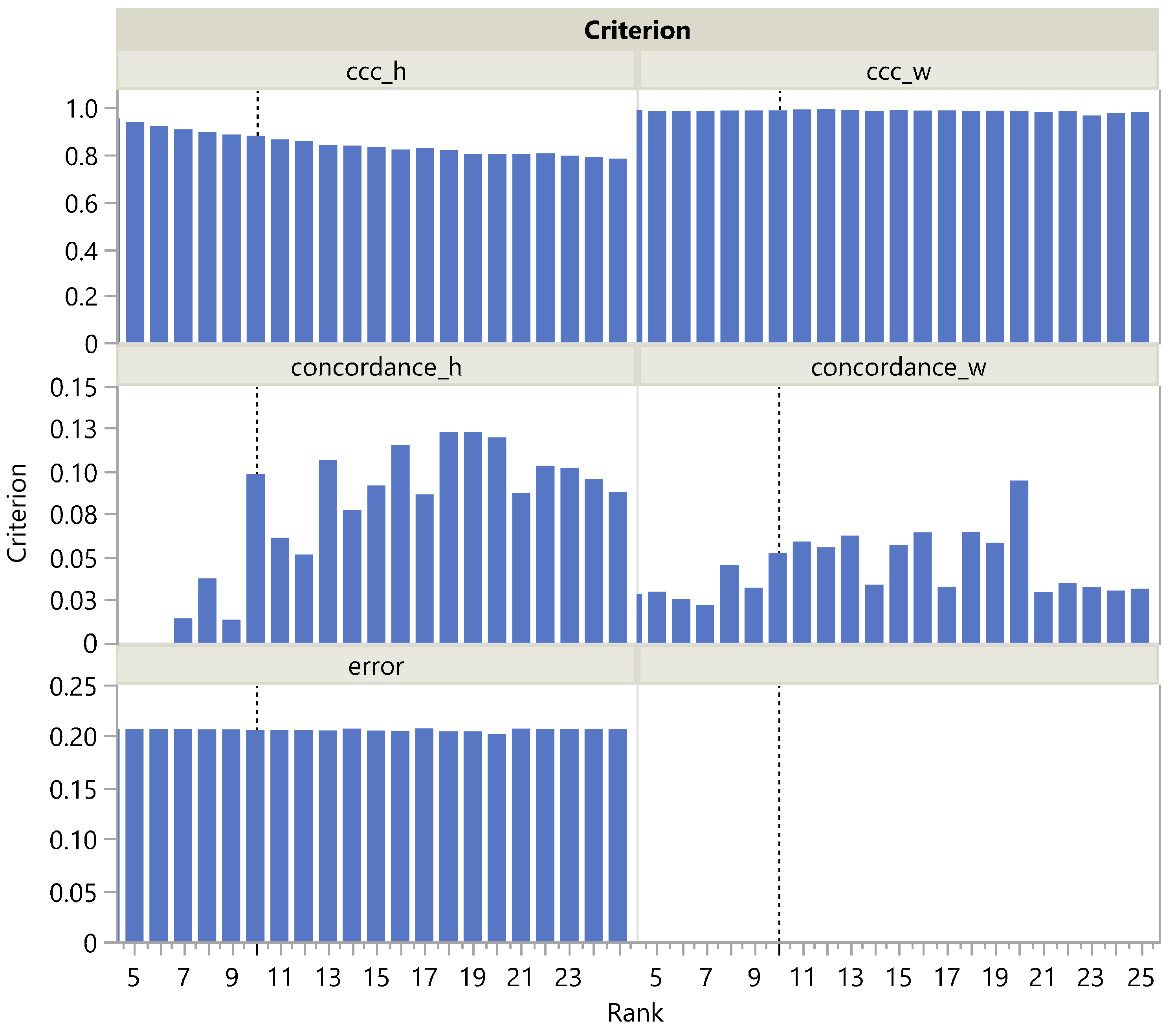
Looking more closely at the MNIST panel a in Figure 3, we see that is actually maximal at rank 20 and then steadily decreases, which is reflected in a steady increase in the corresponding CUSUM chart. This could be easily explained by the presence of archetypal handwriting variants of the same figure. The term being nearly constant (Figure 4), only the term plays a role in correctly estimating the rank as being 10, unlike , which slowly decreases with rank in the H dimension and remains almost constant in the W dimension. It is noteworthy that is always quite low, ranging from 0 to 0.15. This may be due to the fact that even a single individual never reproduces exactly the same figure by hand, resulting in a high amount of noise in the MNIST dataset. Nevertheless, increases significantly at rank 10. This illustrates the robustness of rank selection using in the presence of noise.

Figure 4.
, , and as a function of the rank in the MNIST dataset. The vertical dotted line corresponds to the actual rank.
For the Swimmer dataset, it is noteworthy that is stable in the H dimension, without a maximum at rank 17, and is steadily decreasing in the W dimension (Figure 5). Nevertheless, correctly selects the rank as being 17, thanks to the term in the denominator, which is suppressed at rank 17, since an exact solution can be found. In contrast, has a clear maximum at rank 17 in both dimensions W and H, so both the numerator and denominator contribute to the success of .
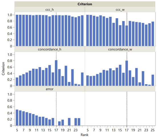
Figure 5.
and as a function of the rank in the Swimmer dataset. The vertical dotted line corresponds to the actual rank.
3.3. Computational Performance
The maximum number of iterations (denoted by ) of NMF updates plays a crucial role in the computational performance of the algorithm. This tuning parameter needs to be set high enough to ensure a stable solution for the reference components obtained with the NNDSVD initialization, from which the approximation error is calculated. In contrast, NMF runs used to correlate random and reference components () or to co-cluster observations or features () need not be as precise. Therefore, using the Swimmer dataset, we compared the performance of and using different values for the maximum number of NMF updates following random initialization (Table 2). The selected rank remained correct down to for both criteria. The difference between the computation times was small, less than one minute, which is due to the simple and sparse structure of the matrix studied. However, the time required to compute was consistently higher than for , and three times higher at , due to the computational complexity of the consensus matrix and linkage calculations.

Table 2.
Performance (in seconds) of and as a function of the maximum number of NMF updates.
The same experiment applied to our simulated data sets using the criterion showed that the distribution of the rank estimation error appears less and less skewed as the maximum number of iterations increases (Figure 6). A maximum number of 50 updates appears to be a reasonable choice.
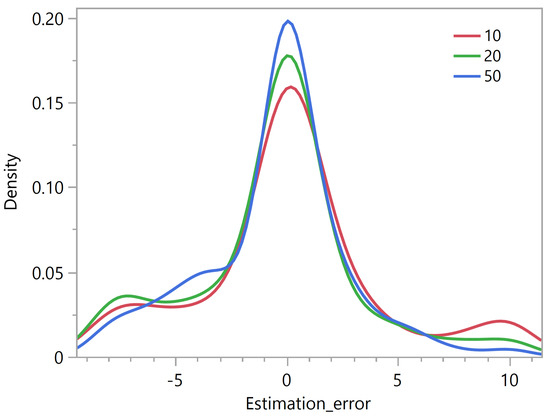
Figure 6.
Rank estimation error using the criterion as a function of the maximum number of NMF updates.
All calculations for this article were performed using the scikit-learn NMF package (https://scikit-learn.org/stable/modules/generated/sklearn.decomposition.NMF.html, accessed on 28 September 2023).
4. Conclusions
In this paper, we have introduced a simulation framework that allowed us to generate a broad class of matrices in terms of shape, correlation structure, and sparsity. Based on these artificial matrices and public datasets, we evaluated the performance of rank selection criteria that exploit the stochastic nature of NMF estimates. An automatic evaluation on a very large set of artificial matrices was made possible by a simple algorithm inspired by CUSUM charts to determine which rank to select based on the screeplot of the criterion versus the tentative ranks.
Given the wide use and acceptance of the cophenetic correlation coefficient criterion among data scientists, the fact that this criterion appears significantly biased toward the selection of lower ranks was a surprising finding. Considering its ratio to the approximation error , the distribution of the rank estimation error appears less skewed, but still biased, albeit in the opposite direction. Strikingly, only on the public Swimmer dataset succeeds in selecting the correct rank, unlike .
We have also proposed a new criterion, , that outperforms on both public and simulated datasets, both in its original form and in its ratio to the approximation form. In addition, we have shown that rank determination using is up to three times faster than with .
This work focuses on metrics that rely on the stochastic nature of the NMF estimates, as is the case for and . The relatively good performance of on synthetic matrices with orthogonal underlying factors [9], led us to use it as a reference metric when introducing the criterion. Non-stochastic metrics, such as those from [14] and many others, could have also been considered for comparative purposes. We have not explored that in the context of our current work because our research aims were: (i) to evaluate the performance of and on a larger class of synthetic matrices with non-orthogonal underlying factors (with the matrices being generated by using a novel simulation framework, which is one of the contributions of our study), and (ii) to evaluate the impact of combining a particular metric with the approximation error by considering their ratio. Nevertheless, the evaluation of the performance of other metrics on this larger class of matrices is an important area for future work.
Incidentally, this study shows that the NNDSVD initialization not only converges faster, as contended by Boustidis et al. [20], but also provides reliable NMF estimates, in the sense that they can be used as a reference when calculating the deviation of estimates obtained with a random initialization.
The fact that the error term in the MNIST dataset does not decrease with rank highlights the limitation of matrix generation using known factors and adding noise, where the error term always tends to decrease with rank. This limitation may explain why deep-learning models trained on generated matrices, as in [14], do not generalize well.
Author Contributions
Conceptualization, P.F. and C.G.; methodology, P.F., C.G. and N.M.; software, P.F. and C.G.; validation, P.F., C.G. and N.M.; formal analysis, P.F., C.G.; investigation, P.F., C.G., N.M. and G.L.; data curation, C.G. and N.M.; writing—original draft preparation, P.F., C.G. and N.M.; writing—review and editing, P.F., C.G., N.M. and G.L.; visualization, P.F., C.G. and N.M. All authors have read and agreed to the published version of the manuscript.
Funding
This research received no external funding.
Data Availability Statement
The public datasets and notebooks used for this work are available at the following link: https://github.com/Advestis/nmf-rank-determination, accessed on 28 September 2023.
Conflicts of Interest
The authors declare no conflict of interest.
Abbreviations
The following abbreviations are used in this manuscript:
| AIC | Akaike Information Criterion |
| ALL | Acute Lymphoblastic Leukemia |
| AML | Acute Myeloid Leukemia |
| BIC | Bayesian Information Criterion |
| Cophenetic Correlation Coefficient | |
| NIR | Near Infrared |
| NMF | Non-negative Matrix Factorization |
| NNDSVD | Non-negative Double Singular Value Decomposition |
| PCA | Principal Component Analysis |
| s | Seconds |
| SVD | Singular Value Decomposition |
References
- Lee, D.D.; Seung, H.S. Learning the parts of objects by non-negative matrix factorization. Nature 1999, 401, 788–791. [Google Scholar] [CrossRef] [PubMed]
- Cichocki, A.; Zdunek, R.; Phan, A.H.; Amari, S.I. Nonnegative Matrix and Tensor Factorizations: Applications to Exploratory Multi-Way Data Analysis and Blind Source Separation; John Wiley & Sons: Hoboken, NJ, USA, 2009. [Google Scholar]
- Gillis, N. The Why and How of Nonnegative Matrix Factorization. arXiv 2014, arXiv:stat.ML/1401.5226. [Google Scholar]
- Kim, P.M.; Tidor, B. Subsystem identification through dimensionality reduction of large-scale gene expression data. Genome Res. 2003, 13, 1706–1718. [Google Scholar] [CrossRef]
- Fogel, P.; Gaston-Mathé, Y.; Hawkins, D.M.; Fogel, F.; Luta, G.; Young, S.S. Applications of a Novel Clustering Approach Using Non-Negative Matrix Factorization to Environmental Research in Public Health. Int. J. Environ. Res. Public Health 2016, 13, 509. [Google Scholar] [CrossRef] [PubMed]
- Griffin, S.R.; Biechele-Speziale, J.A.; Smith, C.J.; You-Dow, X.; White, J.K.; Zhang, S.W.; Novak, J.; Liu, Z.; Simpson, G.J. Iterative Non-Negative Matrix Factorization Filter for Blind Deconvolution in Photon/Ion Counting. Anal. Chem. 2019, 91, 5286–5294. [Google Scholar] [CrossRef] [PubMed]
- Boldina, G.; Fogel, P.; Rocher, C.; Bettembourg, C.; Luta, G.; Augé, F. A2Sign: Agnostic Algorithms for Signatures—A universal method for identifying molecular signatures from transcriptomic datasets prior to cell-type deconvolution. Bioinformatics 2021, 38, 1015–1021. [Google Scholar] [CrossRef]
- Egger, R.; Yu, J. A Topic Modeling Comparison Between LDA, NMF, Top2Vec, and BERTopic to Demystify Twitter Posts. Front. Sociol. 2022, 7, 886498. [Google Scholar] [CrossRef]
- Maisog, J.M.; DeMarco, A.T.; Devarajan, K.; Young, S.; Fogel, P.; Luta, G. Assessing Methods for Evaluating the Number of Components in Non-Negative Matrix Factorization. Mathematics 2021, 9, 2840. [Google Scholar] [CrossRef]
- Brunet, J.P.; Tamayo, P.; Golub, T.R.; Mesirov, J.P. Metagenes and molecular pattern discovery using matrix factorization. Proc. Natl. Acad. Sci. USA 2004, 101, 4164–4169. [Google Scholar] [CrossRef]
- Squires, S.; Prügel-Bennett, A.; Niranjan, M. Rank Selection in Nonnegative Matrix Factorization using Minimum Description Length. Neural Comput. 2017, 29, 2164–2176. [Google Scholar] [CrossRef]
- Owen, A.B.; Perry, P.O. Bi-cross-validation of the SVD and the nonnegative matrix factorization. Ann. Appl. Stat. 2009, 3, 564–594. [Google Scholar] [CrossRef]
- Kanagal, B.; Sindhwani, V. Rank Selection in Low-Rank Matrix Approximations: A Study of Cross-Validation for NMFs. 2010. Available online: https://api.semanticscholar.org/CorpusID:13221897 (accessed on 28 September 2023).
- Nebgen, B.T.; Vangara, R.; Hombrados-Herrera, M.A.; Kuksova, S.; Alexandrov, B.S. A neural network for determination of latent dimensionality in non-negative matrix factorization. Mach. Learn. Sci. Technol. 2020, 2, 025012. [Google Scholar]
- Devarajan, K. Nonnegative Matrix Factorization: An Analytical and Interpretive Tool in Computational Biology. PLoS Comput. Biol. 2008, 4, e1000029. [Google Scholar] [CrossRef] [PubMed]
- Yang, X.; Wu, W.; Xin, X.; Su, L.; Xue, L. Adaptive factorization rank selection-based NMF and its application in tumor recognition. Int. J. Mach. Learn. Cybern. 2021, 12, 2673–2691. [Google Scholar] [CrossRef]
- Cichocki, A.; Zdunek, R. Multilayer Nonnegative Matrix Factorization Using Projected Gradient Approaches. Int. J. Neural Syst. 2007, 17, 431–446. [Google Scholar] [CrossRef]
- Gaujoux, R.; Seoighe, C. Using the Package NMF. BMC Bioinform. 2010, 11, 367. [Google Scholar]
- Zitnik, M.; Zupan, B. NIMFA: A Python Library for Nonnegative Matrix Factorization. J. Mach. Learn. Res. 2012, 13, 849–853. [Google Scholar]
- Boutsidis, C.; Gallopoulos, E. SVD based initialization: A head start for nonnegative matrix factorization. Pattern Recognit. 2008, 41, 1350–1362. [Google Scholar] [CrossRef]
- Golub, T.R.; Slonim, D.K.; Tamayo, P.; Huard, C.; Gaasenbeek, M.; Mesirov, J.P.; Coller, H.A.; Loh, M.L.; Downing, J.R.; Caligiuri, M.A.; et al. Molecular classification of cancer: Class discovery and class prediction by gene expression monitoring. Science 1999, 286, 531–537. [Google Scholar] [CrossRef]
- Fogel, P.; Young, S.S.; Hawkins, D.M.; Ledirac, N. Inferential, robust non-negative matrix factorization analysis of microarray data. Bioinformatics 2007, 23, 44–49. [Google Scholar] [CrossRef]
- Ellekjær, M.R.; Isaksson, T.; Solheim, R. Assessment of Sensory Quality of Meat Sausages Using Near Infrared Spectroscopy. J. Food Sci. 1994, 59, 456–464. [Google Scholar] [CrossRef]
- Donoho, D.L.; Stodden, V. When Does Non-Negative Matrix Factorization Give a Correct Decomposition into Parts? Adv. Neural Inf. Process. Syst. 2003, 16, 1141–1148. [Google Scholar]
- LeCun, Y.; Cortes, C. The Mnist Database of Handwritten Digits. 2005. Available online: https://www.semanticscholar.org/paper/The-mnist-database-of-handwritten-digits-LeCun-Cortes/dc52d1ede1b90bf9d296bc5b34c9310b7eaa99a2 (accessed on 28 September 2023).
- Hoyer, P.O. Non-negative matrix factorization with sparseness constraints. J. Mach. Learn. Res. 2004, 5, 1457–1469. [Google Scholar]
- Potluru, V.A. Block Coordinate Descent for Sparse NMF. arXiv 2013, arXiv:1301.3527. [Google Scholar]
- Ge, R. Tensor Methods in Machine Learning. Off Convex Path. 2015. Available online: https://www.offconvex.org/2015/12/17/tensor-decompositions/ (accessed on 28 September 2023).
- Jayalath, K.P.; Turner, J. Analysis of Means (ANOM) Concepts and Computations. Appl. Appl. Math. Int. J. 2021, 16, 5. [Google Scholar]
Disclaimer/Publisher’s Note: The statements, opinions and data contained in all publications are solely those of the individual author(s) and contributor(s) and not of MDPI and/or the editor(s). MDPI and/or the editor(s) disclaim responsibility for any injury to people or property resulting from any ideas, methods, instructions or products referred to in the content. |
© 2023 by the authors. Licensee MDPI, Basel, Switzerland. This article is an open access article distributed under the terms and conditions of the Creative Commons Attribution (CC BY) license (https://creativecommons.org/licenses/by/4.0/).

