Bayesian Analysis of Unit Log-Logistic Distribution Using Non-Informative Priors

Abstract

The unit log-logistic distribution is a suitable choice for modeling data enclosed within the unit interval. In this paper, estimating the parameters of the unit-log-logistic distribution is performed through a Bayesian approach with non-informative priors. Specifically, we use Jeffreys, reference, and matching priors, with the latter depending on the interest parameter. We derive the corresponding posterior distributions and validate their propriety. The Bayes estimators are then computed using Markov Chain Monte Carlo techniques. To assess the finite sample performance of these Bayes estimators, we conduct Monte Carlo simulations, evaluating their mean squared errors and their coverage probabilities of the highest posterior density credible intervals. Finally, we use these priors to obtain estimations and credible sets for the parameters in an example of a real data set for illustrative purposes.

1. Introduction

Data sets in various fields, including environmental science, biology, epidemiology, and finance, often exhibit values within a specific range, frequently falling within the bounded unit interval $(0,1)$. Examples of such data include proportions in environmental studies, infection rates in epidemiology, and profit margins in finance. To model this type of data, traditional continuous probability distributions like the unit uniform, beta, Johnson SB [1], and Kumaraswamy [2] distributions can be applied in theory. However, it is important to recognize that these conventional distributions may prove ineffective in modeling such data, often due to skewness or extreme events. Consequently, this challenge has stimulated numerous researchers to explore new, more flexible unit distributions that do not require the introduction of additional parameters. More specifically, let $X>0$ be a random variable with a probability density function (pdf) denoted as $f(x,\theta )$. It can be shown that $y=exp(-x)$ follows a probability distribution denoted as $f(y,\theta )$, with y lying within the interval $(0,1)$. This method of transformation has been widely employed in the introduction of various unit distributions by numerous authors. Some noteworthy recent examples include the work of Ghitany et al. [3], who introduced the unit-inverse Gaussian distribution, Mazucheli et al. [4], who proposed the unit-Gompertz distribution, Mazucheli et al. [5], who investigated the unit-Weibull distribution, Ribeiro–Reis [6], who studied the unit log-logistic distribution, Korkmaz and Chesneau [7], who conducted research into the unit Burr-XII distribution, Korkmaz and Korkmaz [8], who proposed the log-log distribution, and finally Najwan et al. [9], who investigated the inverse unit Teissier distribution, among other distributions.

The two-parameter unit log-logistic (ULL) distribution with parameters, $\lambda$, and $\beta$ is defined through the following probability density function

$$\begin{array}{c}\hfill f(x;\lambda ,\beta )=\frac{\lambda \beta {\left\{-ln\left(x\right)\right\}}^{\beta -1}}{x{\left(1+\lambda {\left\{-ln\left(x\right)\right\}}^{\beta }\right)}^2},0<x<1,\end{array}$$

(1)

where $\lambda ,\beta >0$ are unknown parameters. Notice that the parameter $\lambda$ is no longer considered a scale parameter, in contrast to the ULL distribution in Ribeiro–Reis [6], where $\lambda$ serves as a scale parameter.

Estimating the parameters of the ULL distribution is typically achieved through a maximum likelihood (ML) estimation approach. It is worth noting that there has been limited exploration of Bayesian estimation techniques for unit distributions, and, in particular, no prior work has addressed Bayesian analysis for ULL distribution parameters.

In this paper, we introduce a non-informative Bayesian analysis method for these parameters. Notably, among non-informative priors, the Jeffreys prior stands out due to its many appealing properties, such as invariance under one-to-one transformations and computational simplicity. However, this prior may lack robustness when dealing with high-dimensional distributions. On the other hand, there exist two alternative approaches for deriving non-informative priors. One is the reference prior that is originally proposed in [10,11], and formally defined in [12] for one block of parameters. It should be noted that the reference prior separates the parameters into different ordering groups of interest. The other approach considers the concept of probability matching priors for the parameters of interest first introduced by [13]. Notably, these prior distributions are designed in a way that the posterior probabilities within specified intervals match with their corresponding coverage probabilities; see, for example, [14].

The motivation for choosing non-informative priors lies in their capacity to avoid incorporating much information about the model parameters. Additionally, these priors are constructed based on sound scientific principles. In contrast, subjective priors, while reasonable when historical or reliable data are available for eliciting the accompanying hyperparameters to these priors, may be impractical in situations where such data are unavailable.

The remainder of the paper is organized as follows. In Section 2, we provide some specific preparation steps for formulating noninformative priors. Objective priors for the parameter of interest $\lambda$ are given in Section 3. In Section 4, we introduce objective priors when the parameter of interest is $\beta .$ The Posterior predictive assessment of the model is given in Section 5. In Section 6, a simulation study is carried out to assess the finite properties of Bayesian estimators using the noninformative priors. The suggested Bayesian approach is employed to analyze a real data set given in Section 7. In Section 8, we present some conclusions.

2. Formulating Noninformative Priors: Preparation Steps

In this section, our focus is on introducing non-informative priors for the parameters of the unit log-logistic distribution using principle rules. Specifically, we derive Jeffreys’s prior, reference priors, and probability matching priors. It is important to see that the development of these priors is significantly dependent on the Fisher information matrix. So, we report here the Fisher information matrix for the unit log-logistic distribution.

$$\begin{array}{c}\hfill \mathbf{I}(\lambda ,\beta )=\left(\begin{array}{cc}\frac{1}{3{\lambda }^2}& -\frac{ln\left(\lambda \right)}{3\lambda \beta }\\ & \\ -\frac{ln\left(\lambda \right)}{3\lambda \beta }& \frac{3{ln}^2\left(\lambda \right)+({\pi }^2+3)}{9{\beta }^2}\end{array}\right).\end{array}$$

(2)

2.1. Jeffreys-Rule Prior

Jeffreys’ prior is a common choice for non-informative priors in Bayesian statistics due to its fascinating properties. One important feature is its ability to yield a prior distribution that remains invariant under reparameterization, thus ensuring consistency across various parameterizations. The Jeffreys prior for the parameters $(\lambda ,\beta )$ is defined as proportional to the square root of the determinant of the Fisher information matrix.

Theorem 1.

The Jeffreys prior for the parameters $(\lambda ,\beta )$ of the ULL($\lambda ,\beta$) (2) has the following form

$$\begin{array}{c}\hfill {\pi }_J(\lambda ,\beta )\propto \frac{1}{\lambda \beta }.\end{array}$$

(3)

2.2. Useful Results in Establishing Reference and Matching Priors

Here, we present some results about the reference and matching priors. These results may facilitate in obtaining such priors.

Theorem 2.

Consider a probability density function, $f\left(\mathbf{x}\right|\gamma )$ with $\mathbf{x}\in {\mathbb{R}}^n$ and $\gamma ={({\gamma }_1,\dots ,{\gamma }_p)}^{{}^{\prime }}.$ Fix i, let ${\gamma }_i$ be the parameter of interest and ${\gamma }_{(-i)}={({\gamma }_1,\dots ,{\gamma }_{i-1},{\gamma }_{i+1},\dots ,{\gamma }_p)}^t$ be the vector of nuisance parameters of length $p-1.$ Assume that the Fisher information matrix per unit observation is

$$\mathbf{I}\left(\gamma \right)=diag\left(g_1\left({\gamma }_1\right)h_1\left({\gamma }_{(-1)}\right),g_2\left({\gamma }_2\right)h_2\left({\gamma }_{(-2)}\right),\dots ,g\left({\gamma }_p\right)h\left({\gamma }_{(-p)}\right)\right),$$

where for $i=1,\dots ,p,$ $g_i$ is a positive function of ${\gamma }_i$ and $h_i$ is a positive function of ${\gamma }_{(-i)}.$ Then, for any preferred parameter of interest and any ordering of the nuisance parameters, the one-at-a-time reference prior has the following form

$$\pi \left(\gamma \right)\propto \prod _i^p{g}_i^{1/2}\left({\gamma }_i\right).$$

Proof. 

See Datta and Ghosh [15].    □

Theorem 3.

Consider the assumptions of Theorem 2. Suppose that the Fisher information matrix per unit of observation is diagonal, but not necessarily that the components of the matrix can be factorized, i.e.,

$$\mathbf{I}\left(\gamma \right)=diag\left({\mathbf{I}}_{11}\left(\gamma \right),\dots ,{\mathbf{I}}_{pp}\left({\gamma }_p\right)\right),$$

where ${\mathbf{I}}_{kk}\left(\gamma \right)$ is the $(k,k)$th-element of $\mathbf{I}.$ Then, the matching prior for the parameter of interest ${\gamma }_k$ is

$${\pi }_M\left(\gamma \right)\propto {\mathbf{I}}_{kk}^{1/2}\left(\gamma \right)g\left({\gamma }_{(-k)}\right).$$

Proof. 

See Tibshirani [16].    □

3. Objective Priors for the Parameter $\mathit{\lambda }$

In this Section, we develop reference and matching priors for the parameter of interest, $\lambda .$ Note that the Fisher information is not a diagonal matrix, implying that the parameters are not orthogonal. So, our task now is to find a 1-1 transformation from $(\lambda ,\beta )$ onto $(\psi ,\tau )$ so that the new Fisher information matrix is a diagonal matrix. The following lemma reports the required transformation.

Lemma 1.

Considering the unit log-logistic distribution in (1) along with the Fisher information matrix in (2), then the transformation $\psi =\lambda$ and $\tau =\beta /\sqrt{3{ln}^2\left(\lambda \right)+(3+{\pi }^2)}$ yields a diagonal Fisher information matrix, given as

$${\mathbf{H}}^{\lambda }(\psi ,\tau )=diag\left(\frac{3+{\pi }^2}{3{\psi }^2(3{ln}^2\left(\psi \right)+3+{\pi }^2)},\frac{3{ln}^2\left(\psi \right)+3+{\pi }^2}{9{\tau }^2}\right).$$

Here, ${\mathbf{H}}^{\lambda }(\psi ,\tau )$ denotes the diagonal Fisher information matrix, considering that the parameter of interest, $\lambda .$

Proof. 

The Jacobian of transformation, $(\lambda ,\beta )⟶(\psi ,\tau )$, matrix is

$$\mathbf{G}=\frac{\partial (\lambda ,\beta )}{\partial (\psi ,\tau )}=\left(\begin{array}{cc}1& 0\\ & \\ {\displaystyle \frac{3\tau ln\left(\psi \right)}{\psi \sqrt{3{ln}^2\left(\psi \right)+3+{\pi }^2}}}& \sqrt{3{ln}^2\left(\psi \right)+3+{\pi }^2}\end{array}\right).$$

So, the new Fisher information matrix in terms of $\psi$ and $\tau$ is obtained via ${\mathbf{H}}^{\lambda }(\psi ,\lambda )={\mathbf{G}}^t\mathbf{I}\mathbf{G}$.    □

3.1. Reference Prior

Following the preparation steps outlined along with the results presented in Section 3, we are now in a position to derive the reference prior for the parameter of interest; $\psi$

Theorem 4.

For the ordering group $(\lambda ,\beta )$, the reference prior is given by

$$\begin{array}{c}\hfill {\pi }_R(\lambda ,\beta )\propto \frac{1}{\lambda \beta \sqrt{3{ln}^2\left(\lambda \right)+3+{\pi }^2}}.\end{array}$$

(4)

Proof. 

The Fisher information presented in Lemma 1 exhibits a diagonal matrix structure. Observe that ${\mathbf{H}}^{\lambda }(\psi ,\tau )=diag\left(g_1\left(\psi \right)h_1\left(\tau \right),g_2\left(\tau \right)h_2(\psi ,\tau )\right)$ with

$$g_1\left(\psi \right)=\frac{1}{{\psi }^2(3{ln}^2\left(\psi \right)+3+{\pi }^2)},h_1\left(\tau \right)=\frac{3+{\pi }^2}{3},g_2\left(\tau \right)=\frac{1}{9{\tau }^2},$$

and $h_2\left(\psi \right)=3{ln}^2\left(\psi \right)+3+{\pi }^2.$ On applying Theorem 2, the reference prior associated with the parameters $(\psi ,\tau )$ can be expressed as:

$$\begin{array}{c}\hfill {\pi }_R(\psi ,\tau )\propto g_1^{1/2}\left(\psi \right)·g_2^{1/2}\left(\tau \right)=\frac{1}{\tau \psi \sqrt{3{ln}^2\left(\psi \right)+3+{\pi }^2}}.\end{array}$$

(5)

Upon a transformation back to the original parameters $(\lambda ,\beta )$ and taking into consideration the Jacobian of the transformation from $(\psi ,\tau )$ to $(\lambda ,\beta )$, which is given by $1/\sqrt{3{ln}^2\left(\lambda \right)+3+{\pi }^2}$, it is evident that the reference prior follows the form specified in (4).    □

3.2. Probability Matching Priors

Let $\mathbf{X}=(X_1,\dots ,X_n)$ be a random sample from the unit log-logistic distribution in (1). Given a prior $\pi =\pi (\lambda ,\beta )$, denote ${\lambda }^{1-\alpha }(\pi ;\mathbf{X})$ as the $(1-\alpha )$th quantile of the marginal posterior of $\lambda$, i.e.,

$$\stackrel{\pi }{Pr}\left\{\lambda \le {\lambda }^{1-\alpha }(\pi ;\mathbf{X})|\mathbf{X}\right\}=1-\alpha ,$$

(6)

where $\beta$ is the nuisance parameter and ${Pr}^{\pi }\left\{.|\mathbf{X}\right\}$ is the posterior probability measure. We seek for priors $\pi$ such that the following equation holds for all $\alpha \in (0,1),$

$$\begin{array}{c}\hfill \underset{\lambda }{Pr}\{\lambda \le {\lambda }^{1-\alpha }(\pi ;\mathbf{X})\}=1-\alpha +o\left(n^{-1}\right),\end{array}$$

(7)

where ${Pr}_{\lambda }\{.\}$ is the probability distribution measure of $\mathbf{X}$ indexed by the parameter $\lambda .$ A prior that satisfies Equations (6) and (7) is referred as a second-order probability matching when the parameter of interest is $\lambda$ The following theorem establishes the required prior.

Theorem 5.

For the parameter of interest λ and the nuisance parameter $\beta ,$ the second-order probability matching has the following form

$$\begin{array}{c}\hfill {\pi }_M(\psi ,\tau )\propto \frac{1}{\psi \left(3{ln}^2\left(\psi \right)+3+{\pi }^2\right)}·g\left(\tau \right),\end{array}$$

(8)

where $g(·)$ represents an arbitrary positive function.

Proof. 

We have that

$$\begin{array}{cc}\hfill {\mathbf{H}}^{\lambda }(\psi ,\lambda )& =diag\left({\mathbf{H}}_{\psi \psi }^{\lambda },{\mathbf{H}}_{\tau \tau }^{\lambda }\right)\hfill \\ \hfill & :=diag\left(\frac{3+{\pi }^2}{3{\psi }^2(3{ln}^2\left(\psi \right)+3+{\pi }^2)},\frac{3{ln}^2\left(\psi \right)+3+{\pi }^2}{9{\tau }^2}\right)\hfill \end{array}$$

Upon application of Theorem 3, the form of the matching prior should take the following form

$${\pi }_M(\psi ,\tau )\propto \sqrt{{\mathbf{H}}_{\psi \psi }^{\lambda }}·g\left(\tau \right)\propto \frac{1}{\sqrt{{\psi }^2(3{ln}^2\left(\psi \right)+3+{\pi }^2)}}·g\left(\tau \right).$$

   □

Theorem 6.

The Jeffreys prior ${\pi }_J$ is not a second-order probability matching prior.

Proof. 

The Jeffreys prior in terms of $\psi$ and $\tau$ is ${\pi }_J(\psi ,\tau )\propto 1/\psi \tau .$ Clearly, this prior can not be written in the form of general matching prior, which is given in (8). Since the Jeffreys is invariant under 1-1 transformation, implying that the Jeffreys prior in (3) is not a second-matching prior.    □

Theorem 7.

The reference prior in (4) is a second-matching prior.

Proof. 

By taking $g\left(\tau \right)=1/\tau$ in (8) resulting the reference; ${\pi }_R(\psi ,\tau )$, which is given in (5).    □

3.3. Propriety of Posterior Distributions

It is evident that the priors derived in Section 2 are all improper. Therefore, it becomes necessary to assess the propriety of the resulting posterior distributions that arise from these priors. Here, we consider a general class of priors

$$\begin{array}{c}\hfill \pi (\lambda ,\beta )\propto {\lambda }^{-1}{\beta }^{-b}\frac{1}{\sqrt{3{ln}^2\left(\lambda \right)+3+{\pi }^2}},\end{array}$$

(9)

where $b>0.$

Theorem 8.

The posterior distribution under the general prior in (9) is proper whenever $n>b$.

Proof. 

The joint posterior distribution of $\lambda$ and $\beta$ under the prior (9) given $\mathbf{x}$ is given by

$$\begin{array}{cc}\hfill \pi (\lambda ,\beta |\mathbf{x})& \propto \frac{{\lambda }^{n-1}{\beta }^{n-b}}{\sqrt{3{ln}^2\left(\lambda \right)+3+{\pi }^2}}\prod _{i=1}^n\left(\frac{{\left\{-ln\left(x_i\right)\right\}}^{\beta }}{{\left(1+\lambda {\left\{-ln\left(x_i\right)\right\}}^{\beta }\right)}^2}\right)\hfill \end{array}$$

(10)

Let $h_{i,1}(\lambda ,\beta ):={\left\{-ln\left(x_i\right)\right\}}^{\beta }{\left(1+\lambda {\left\{-ln\left(x_i\right)\right\}}^{\beta }\right)}^{-2},$ for $i=1,\dots ,n,$ and

$$h_2(\lambda ,\beta ):={\left\{-ln\left(x_{\left(n\right)}\right)\right\}}^{\beta }{\left(1+\lambda {\left\{-ln\left(x_{\left(1\right)}\right)\right\}}^{\beta }\right)}^{-2},$$

where $x_{\left(n\right)}=max(x_1,\dots ,x_n)$ and $x_{\left(1\right)}=min(x_1,\dots ,x_n).$ For $\lambda ,\beta >0,$ we have that $0<h_2(\lambda ,\beta )<h_{i1}(\lambda ,\beta )<1.$ Therefore, there exists positive constants, $c_1,\dots ,c_n$ such that

$$h_{i,1}(\lambda ,\beta )<c_i·h_2(\lambda ,\beta ),i=1,\dots ,n.$$

Putting $c={\prod }_{i=1}^n{c}_i,$ it then follows that

$$\begin{array}{cc}\hfill \pi (\lambda ,\beta |\mathbf{x})& \le c·\frac{{\lambda }^{n-1}{\beta }^{n-b}}{\sqrt{3{ln}^2\left(\lambda \right)+3+{\pi }^2}}\frac{{\left\{-ln\left(x_{\left(n\right)}\right)\right\}}^{\beta n}}{{\left(1+\lambda {\left\{-ln\left(x_{\left(1\right)}\right)\right\}}^{\beta }\right)}^{2n}}.\hfill \end{array}$$

(11)

Observe that the function

$$g\left(\lambda \right):=\frac{1}{\sqrt{3{ln}^2\left(\lambda \right)+3+{\pi }^2}}$$

attains its maximum at $\lambda =1.$ It then follows that $g\left(\lambda \right)\le {sup}_{\lambda }g\left(\lambda \right)=1/\sqrt{3+{\pi }^2}.$ So, the joint posterior distribution in (11) can be displayed as follows

$$\begin{array}{cc}\hfill \pi (\lambda ,\beta |\mathbf{x})& \le d·{\lambda }^{n-1}{\beta }^{n-b}\frac{{\left\{-ln\left(x_{\left(n\right)}\right)\right\}}^{\beta n}}{{\left(1+\lambda {\left\{-ln\left(x_{\left(1\right)}\right)\right\}}^{\beta }\right)}^{2n}},\hfill \end{array}$$

where $d>0.$ Thus,

$$\begin{array}{cc}\hfill {\int }_0^{\infty }{\int }_0^{\infty }\pi (\lambda ,\beta |\mathbf{x})\mathrm{d}\lambda \mathrm{d}\beta & \propto d·{\int }_0^{\infty }{\int }_0^{\infty }{\lambda }^{n-1}{\beta }^{n-b}\frac{{\left\{-ln\left(x_{\left(n\right)}\right)\right\}}^{\beta n}}{{\left(1+\lambda {\left\{-ln\left(x_{\left(1\right)}\right)\right\}}^{\beta }\right)}^{2n}}\mathrm{d}\lambda \mathrm{d}\beta .\hfill \end{array}$$

Let $u=\lambda {\{-ln\left(x\right)\}}^{\beta }$, it then follows that

$$\begin{array}{cc}\hfill {\int }_0^{\infty }{\int }_0^{\infty }\pi (\lambda ,\beta |\mathbf{x})\mathrm{d}\lambda \mathrm{d}\beta & \propto d·{\int }_0^{\infty }{\beta }^{n-b}\frac{{\left\{-ln\left(x_{\left(n\right)}\right)\right\}}^{\beta n}}{{\left\{-ln\left(x_{\left(1\right)}\right)\right\}}^{\beta n}}\left\{{\int }_0^{\infty }\frac{u^{n-1}}{{\left(1+u\right)}^{2n}}\mathrm{d}u\right\}\mathrm{d}\beta \hfill \\ \hfill & =\frac{d·{\Gamma }^2\left(n\right)}{\Gamma \left(2n\right)}{\int }_0^{\infty }{\beta }^{n-b}{e}^{-k·\beta }\mathrm{d}\beta ,\hfill \end{array}$$

where $k:=n·\left(ln[-ln\left(x_{\left(n\right)}\right)]-ln[-ln\left(x_{\left(1\right)}\right)]\right).$ Clearly, the integral in the above inequality is finite provided that $n-b>0,$ yielding that $\pi (\lambda ,\beta |\mathbf{x})$ is proper.    □

Theorem 9.

The posterior distributions under ${\pi }_J$ and ${\pi }_R$ all exhibit finiteness. Furthermore, the means under the corresponding posterior distributions are also finite.

Proof. 

The proof can be analogously established to the proof of Theorem 8.    □

4. Objective Priors for the Parameter $\mathit{\beta }$

In this section, we define the reference and matching priors for the parameter of interest, denoted as $\beta$. To achieve this, we first reorganize the components of the Fisher information matrix as follows:

$$\begin{array}{c}\hfill \mathbf{J}(\beta ,\lambda )=\left(\begin{array}{cc}{\displaystyle \frac{3{ln}^2\left(\lambda \right)+({\pi }^2+3)}{9{\beta }^2}}& -{\displaystyle \frac{ln\left(\lambda \right)}{3\lambda \beta }}\\ & \\ -{\displaystyle \frac{ln\left(\lambda \right)}{3\lambda \beta }}& {\displaystyle \frac{1}{3{\lambda }^2}}\end{array}\right).\end{array}$$

(12)

Given the unattainable 1-1 orthogonal transformation, it is necessary to utilize the generic algorithm provided by [17] for deriving a reference prior when dealing with the parameter of interest, $\beta$, and the nuisance parameter, $\lambda$. Notably, when $\beta$ is independent of the nuisance parameter space, $\lambda \left(\beta \right)=\lambda ,$ the application of this algorithm becomes particularly appealing, as highlighted in the subsequent proposition.

Proposition 1

(Bernardo and Smith [17] (2000, p. 328)). Assuming that the conditions of the algorithm by Bernardo and Smith [17] are satisfied, and under the assumption that the parameter of interest β demonstrates independence from the nuisance parameter space $\Lambda \left(\beta \right)=\lambda$, with the functions $G_{\beta }(\beta ,\lambda )=\frac{det\left(\mathbf{J}\right(\beta ,\lambda \left)\right)}{{\mathbf{J}}_{\lambda \lambda }(\beta ,\lambda )}$ and ${\mathbf{J}}_{\lambda \lambda }(\beta ,\lambda )$ factorizing as provided below:

$$G_{\beta }^{\frac{1}{2}}(\beta ,\lambda )=f_1\left(\beta \right)g_1\left(\lambda \right)and{\mathbf{J}}_{\lambda \lambda }^{\frac{1}{2}}(\beta ,\lambda )=f_2\left(\beta \right)g_2\left(\lambda \right),$$

then the reference prior with respect to the ordered group $(\beta ,\lambda )$ is

$$\pi (\beta ,\lambda )=f_1\left(\beta \right)g_2\left(\lambda \right).$$

Similarly, it is not feasible to obtain a matching prior for the parameter of interest, $\beta$, using Theorem 3, due to the unattainable 1-1 orthogonal transformation. Consequently, we must turn to the approach outlined by Peer and Welch [13], who have provided a general formula for deriving a probability matching prior when dealing with a two-parameter distribution. To elaborate, considering $\beta$ as the parameter of interest, any prior for both $\beta$ and $\lambda$-denoted as $\pi (\beta ,\lambda )$-should satisfy the following partial differential equation:

$$\begin{array}{c}\hfill \frac{\partial }{\partial \lambda }\left\{\frac{{\mathbf{J}}_{\beta \lambda }\pi (\beta ,\lambda )}{{\mathbf{J}}_{\lambda \lambda }\sqrt{K}}\right\}-\frac{\partial }{\partial \beta }\left\{\frac{\pi (\beta ,\lambda )}{\sqrt{K}}\right\}=0,\end{array}$$

(13)

Here, $K={\mathbf{J}}_{\lambda \lambda }^{-1}det\left(\mathbf{J}(\beta ,\lambda )\right)$ provides a second-order probability matching prior.

4.1. Reference Prior

Following the preparation steps outlined above, we are now in a position to derive the reference prior for the parameter of interest; $\beta$

Theorem 10.

For the ordering group $(\beta ,\lambda )$, the reference prior is given by

$$\begin{array}{c}\hfill {\pi }_R(\beta ,\lambda )\propto \frac{1}{\lambda \beta }.\end{array}$$

(14)

Proof. 

On using the Fisher information presented in (12), we have that $G_{\beta }^{\frac{1}{2}}(\beta ,\lambda )\propto \frac{1}{\beta }=f_1\left(\beta \right)g_1\left(\lambda \right),$ where $f_1\left(\beta \right)=1/\beta$ and $g_1\left(\lambda \right)=1.$ Next ${\mathbf{J}}_{\lambda ,\lambda }^{\frac{1}{2}}(\beta ,\lambda )\propto 1/\lambda =f_2\left(\beta \right)g_2\left(\lambda \right),$ where $f_2\left(\beta \right)=1$ and $g_2\left(\lambda \right)=1/\lambda .$ In view of Proposition 1, it follows that the reference prior for the ordered group $(\beta ,\lambda )$ is ${\pi }_R(\beta ,\lambda )\propto \frac{1}{\lambda \beta }$.    □

Remark 1.

Observe that when the parameter of interest is β, the reference prior is equivalent to ${\pi }_J$.

4.2. Probability Matching Priors

Theorem 11.

The general form of the second-order probability matching prior, for the parameter of interest β and the nuisance parameter $\lambda ,$ is

$$\begin{array}{c}\hfill {\pi }_M(\beta ,\lambda )\propto \frac{1}{\lambda {ln}^2\left(\lambda \right)}·Q\left(\frac{\beta }{ln\left(\lambda \right)}\right),\end{array}$$

(15)

where $Q(.)$ is any positive function.

Proof. 

Since the parameter of interest is $\beta$, direct calculations yield the following:

$$\frac{{\mathbf{J}}_{\beta \lambda }\pi (\beta ,\lambda )}{{\mathbf{J}}_{\lambda \lambda }\sqrt{K}}=-\frac{3\lambda ln\left(\lambda \right)}{\sqrt{{\pi }^2+3}}\mathrm{and}\frac{1}{\sqrt{K}}=\frac{3\beta }{\sqrt{{\pi }^2+3}}.$$

Substituting these quantities into the partial differential equation in (13), we find that the required second-order probability matching prior should satisfy the following partial differential equation.

$$\begin{array}{cc}\hfill & -\frac{\partial }{\partial \lambda }\left\{\frac{3\lambda ln\left(\lambda \right)\pi (\beta ,\lambda )}{\sqrt{{\pi }^3+3}}\right\}-\frac{\partial }{\partial \beta }\left\{\frac{3\beta \pi (\beta ,\lambda )}{\sqrt{{\pi }^3+3}}\right\}=0\hfill \end{array}$$

It is not difficult to see that the above partial differential equation reduces to

$$\lambda ln\left(\lambda \right)\frac{\partial \pi (\beta ,\lambda )}{\partial \lambda }+\beta \frac{\partial \pi (\beta ,\lambda )}{\partial \beta }+\left\{2+ln\left(\lambda \right)\right\}\pi (\beta ,\lambda )=0.$$

The general solution of the mentioned partial differential equation can be readily obtained and is equivalent to the one presented in (15).    □

Theorem 12.

Considering the general form of the second-order probability matching prior in (15), the following

$$\begin{array}{cc}\hfill {\pi }_{M_1}(\beta ,\lambda )& \propto \frac{1}{\lambda {\beta }^2}\hfill \end{array}$$

(16)

$$\begin{array}{cc}\hfill {\pi }_{M_2}(\beta ,\lambda )& \propto \frac{1}{\lambda {ln}^2\left(\lambda \right)}\hfill \end{array}$$

(17)

are matching priors.

Proof. 

By taking $Q\left(x\right)=1/x^2$ and $Q\left(x\right)=c>0$, respectively, then we obtain the second-order probability matching priors given in (16) and (17).    □

4.3. Propriety of Posterior Distributions

In this subsection, we investigate the finiteness of the posterior distributions under the developed priors when the parameter of interest is $\beta$. It is of interest to note that the reference prior for this case is precisely equivalent to ${\pi }_J$, ensuring a finite posterior distribution, as guaranteed by Theorem 8. Additionally, the matching prior given via (16) yields a proper posterior distribution, as affirmed by Theorem 8 as well. It remains to check the appropriateness of the posterior distributions under the matching given in (17).

Theorem 13.

The posterior distribution under the matching prior (17) is improper.

Proof. 

The joint posterior distribution under the matching prior in (17) is

$${\pi }_{M_2}(\lambda ,\beta |\mathbf{x})\propto \frac{{\lambda }^{n-1}{\beta }^{n-1}}{\lambda {ln}^2\left(\lambda \right)}\prod _{i=1}^n\left(\frac{{\left\{-ln\left(x_i\right)\right\}}^{\beta }}{{\left(1+\lambda {\left\{-ln\left(x_i\right)\right\}}^{\beta }\right)}^2}\right).$$

Now, we have that

$$\begin{array}{cc}\hfill {\int }_0^{\infty }{\int }_0^{\infty }{\pi }_{M_2}(\lambda ,\beta |\mathbf{x})d\lambda d\beta & \propto {\int }_0^{\infty }{\int }_0^{\infty }\frac{{\lambda }^{n-1}{\beta }^{n-1}}{\lambda {ln}^2\left(\lambda \right)}\prod _{i=1}^n\left\{\frac{{\left\{-ln\left(x_i\right)\right\}}^{\beta }}{{\left(1+\lambda {\left\{-ln\left(x_i\right)\right\}}^{\beta }\right)}^2}\right\}d\lambda d\beta \hfill \\ \hfill & ={\int }_0^{\infty }{\beta }^{n-1}\prod _{i=1}^n{\left\{-ln\left(x_i\right)\right\}}^{\beta }\{{\int }_0^{\infty }\frac{{\lambda }^{n-2}}{{ln}^2\left(\lambda \right)}\hfill \\ \hfill & \prod _{i=1}^n{\left[1+\lambda {\left\{-ln\left(x_i\right)\right\}}^{\beta }\right]}^{-2}d\lambda \}d\beta \hfill \end{array}$$

It is not difficult to see that

$$\begin{array}{cc}\hfill {\int }_0^{\infty }\frac{{\lambda }^{n-2}}{{ln}^2\left(\lambda \right)}\prod _{i=1}^n{\left[{\left(1+\lambda {\left\{-ln\left(x_i\right)\right\}}^{\beta }\right)}^2\right]}^{-1}d\lambda & \ge {\int }_0^1\frac{{\lambda }^{n-2}}{{ln}^2\left(\lambda \right)}\prod _{i=1}^n{\left(1+\lambda {\left\{-ln\left(x_i\right)\right\}}^{\beta }\right)}^{-2}d\lambda \hfill \\ \hfill & \ge A(x_i,\beta ){\int }_0^1\frac{{\lambda }^{n-2}}{{ln}^2\left(\lambda \right)}d\lambda \hfill \\ \hfill & =A(x_i,\beta ){\int }_0^{\infty }\frac{exp\{-(n-1\left)u\right\}}{u^2}du,\hfill \end{array}$$

where $A(x_i,\beta )={\left(1+{\left\{-ln\left(x_i\right)\right\}}^{\beta }\right)}^{-2}.$ Clearly, the integral above diverges for $n\ge 1$, which completes the proof.    □

Remark 2.

Notice that ${\pi }_J$ which is equivalent to the reference prior is not a second-order matching prior.

5. Posterior Predictive Assessment of the Model

After establishing posterior propriety using the developed priors for the parameter of interest, the next step involves evaluating the model’s goodness-of-fit to real data. Among the various Bayesian validation techniques available, one particularly powerful method is the use of posterior predictive checks. These checks involve generating new observations (predictive samples) from the model by sampling from the posterior distribution of the parameters and subsequently comparing these replicates to the observed data via graphical tools. Furthermore, we employ the posterior predictive p-value, originally introduced by [18] and formally defined by [19], as an additional tool for model evaluation. It is important to emphasize that this method involves utilizing a discrepancy measure that does not depend on the unknown parameters. An extension of this approach, which permits the discrepancy measure to depend on the unknown parameters, has been proposed by Gelman et al. [20]. We use the following discrepancy measure which is defined as Bayesian Chi-square residuals and given by

$$\begin{array}{cc}\hfill \mathsf{D}(\mathbf{x};{\theta }_i)& =\sum _{i=1}^n\frac{{\left(x_i-E\left(X_i\right|{\theta }_i)\right)}^2}{Var\left(X_i\right|{\theta }_i)}\hfill \end{array}$$

(18)

where ${\theta }_i=({\lambda }_i,{\beta }_i).$ To compute the posterior predictive p-value, we define, the algorithm

• Input observed data $\mathbf{x}=(x_1,\dots ,x_n)$.
• Sample ${\theta }_k=({\lambda }_k,{\beta }_k)$ from the posterior distribution, considering a specified prior and observed data $\mathbf{x}$ under the specified prior, to obtain a posterior sample.
• For each ${\theta }_k=({\lambda }_k,{\beta }_k),$ generate new observations of the same size of the observed data using the UUL distribution; ${\mathbf{x}}^{\mathrm{rep}}$. This represents a predictive sample.
• Compute the discrepancy measures using the predictive and observed data, respectively $\mathsf{D}({\mathbf{x}}^{\mathrm{rep}},{\theta }_k)$ and $\mathsf{D}(\mathbf{x},{\theta }_k)$.
• Repeat steps 2–4 sufficiently large number of times K.

The posterior predictive p-value is then approximated by

$$\mathsf{PP}p=\frac{\#\left\{\mathsf{D}({\mathbf{x}}^{\mathrm{rep}},{\theta }_k)>=\mathsf{D}(\mathbf{x},{\theta }_k)\right\}}{K}.$$

It is of interest to see that one can produce a scatter plot of $\mathsf{D}({\mathbf{x}}^{\mathrm{rep}},{\theta }_k)$ against $\mathsf{D}(\mathbf{x},{\theta }_k)$ for visualization purposes.

6. Simulation Study

The Bayesian estimators of $\lambda$ and $\beta$ under the various non-informative priors presented in this paper cannot be expressed in a closed-form analytical expression. Furthermore, the marginal posterior densities of $\lambda$ and $\beta$ do not appear to yield well-known probability distributions, and this complicates sampling from the joint posterior distribution of $\lambda$ and $\beta$.

Alternatively, we evaluate the finite sample behavior of the Bayesian estimators for the parameters $\lambda$ and $\beta$, considering the noninformative priors ${\pi }_J$, ${\pi }_R$, and ${\pi }_{M_1}$ discussed in Section 3 and Section 4 by conducting a simulation study using Markov Chain Monte Carlo (MCMC). The study involves generating samples from the ULL distribution (1) using different true parameter values and samples of size $n=10,15,20,30,50,70,100,150$. Subsequently, posterior samples are drawn from the joint posterior distribution of $(\lambda ,\beta )$ using the random-walk Metropolis algorithm, as detailed in [21]. Each chain within the process consisted of 5500 samples after discarding the initial 500 burn-in samples. The entire process is replicated 1000 times. Consequently, we can compute the estimated mean squared error (MSE) and the coverage probability (CP) of credible intervals for the parameters $\lambda$ and $\beta$. The empirical findings concerning the MSEs and CPs for 95% credible intervals are available in Table 1 and Table 2, respectively. Several findings from the study conform to our expectations and are evident, as illustrated in both the tables and Figure 1, Figure 2, Figure 3 and Figure 4.

Table 1. Empirical average MSEs and CPs (within parentheses) of Bayesian estimators for the parameter $\lambda$ under different true of $\beta$ and $\lambda$.

Parameters		n	10	15	20	30	50	70	100	150
$\mathit{\beta }$	$\mathit{\lambda }$
0.8	0.5	${\pi }_{\mathrm{J}}$	0.5010 (0.922)	0.3045 (0.929)	0.2662 (0.924)	0.1936 (0.913)	0.1407 (0.931)	0.1157 (0.931)	0.0989 (0.920)	0.0810 (0.916)
		${\pi }_{\mathrm{R}}$	0.4712 (0.944)	0.2988 (0.940)	0.2653 (0.929)	0.1925 (0.923)	0.1406 (0.941)	0.1158 (0.932)	0.0987 (0.921)	0.0807 (0.917)
	1.5	${\pi }_{\mathrm{J}}$	4.2766 (0.951)	1.3487 (0.954)	1.0293 (0.943)	0.6621 (0.945)	0.4591 (0.952)	0.3675 (0.948)	0.3039 (0.941)	0.2401 (0.932)
		${\pi }_{\mathrm{R}}$	3.3626 (0.954)	1.2351 (0.956)	0.9639 (0.942)	0.6330 (0.949)	0.4472 (0.956)	0.3602 (0.949)	0.3002 (0.941)	0.2379 (0.930)
	3	${\pi }_{\mathrm{J}}$	27.9630 (0.955)	5.5104 (0.956)	3.0399 (0.956)	1.7268 (0.952)	1.1224 (0.956)	0.8870 (0.958)	0.7118 (0.944)	0.5448 (0.944)
		${\pi }_{\mathrm{R}}$	22.4203 (0.948)	4.8432 (0.946)	2.7289 (0.953)	1.6036 (0.946)	1.0762 (0.960)	0.8572 (0.956)	0.6976 (0.954)	0.5365 (0.939)
2	0.5	${\pi }_{\mathrm{J}}$	0.4969 (0.926)	0.3014 (0.941)	0.2624 (0.938)	0.1908 (0.927)	0.1387 (0.940)	0.1138 (0.948)	0.0976 (0.932)	0.0791 (0.932)
		${\pi }_{\mathrm{R}}$	0.4680 (0.949)	0.2964 (0.948)	0.2621 (0.943)	0.1901 (0.933)	0.1389 (0.952)	0.1142 (0.948)	0.0977 (0.936)	0.0791 (0.934)
	1.5	${\pi }_{\mathrm{J}}$	4.2800 (0.951)	1.3429 (0.954)	1.0234 (0.942)	0.6595 (0.948)	0.4550 (0.955)	0.3636 (0.943)	0.2996 (0.943)	0.2367 (0.936)
		${\pi }_{\mathrm{R}}$	3.3496 (0.953)	1.2312 (0.952)	0.9576 (0.944)	0.6303 (0.949)	0.4439 (0.952)	0.3570 (0.950)	0.2958 (0.939)	0.2347 (0.936)
	3	${\pi }_{\mathrm{J}}$	27.8864 (0.952)	5.5294 (0.955)	3.0266 (0.952)	1.7242 (0.953)	1.1189 (0.953)	0.8816 (0.956)	0.7055 (0.948)	0.5395 (0.937)
		${\pi }_{\mathrm{R}}$	22.4256 (0.946)	4.8295 (0.946)	2.7212 (0.948)	1.6032 (0.948)	1.0731 (0.954)	0.8527 (0.956)	0.6910 (0.946)	0.5317 (0.939)
5	0.5	${\pi }_{\mathrm{J}}$	0.4978 (0.928)	0.3015 (0.941)	0.2622 (0.938)	0.1909 (0.926)	0.1388 (0.940)	0.1137 (0.946)	0.0977 (0.931)	0.0792 (0.935)
		${\pi }_{\mathrm{R}}$	0.4679 (0.949)	0.2964 (0.948)	0.2623 (0.942)	0.1901 (0.933)	0.1389 (0.950)	0.1141 (0.947)	0.0977 (0.938)	0.0790 (0.937)
	1.5	${\pi }_{\mathrm{J}}$	4.2751 (0.951)	1.3456 (0.954)	1.0226 (0.943)	0.6600 (0.946)	0.4549 (0.952)	0.3634 (0.946)	0.2995 (0.941)	0.2366 (0.935)
		${\pi }_{\mathrm{R}}$	3.1325 (0.954)	1.2329 (0.954)	0.9577 (0.944)	0.6298 (0.947)	0.4438 (0.951)	0.3572 (0.947)	0.2959 (0.940)	0.2347 (0.935)
	3	${\pi }_{\mathrm{J}}$	28.1580 (0.952)	5.5408 (0.954)	3.0291 (0.952)	1.7246 (0.951)	1.1180 (0.956)	0.8829 (0.958)	0.7051 (0.944)	0.5401 (0.940)
		${\pi }_{\mathrm{R}}$	22.2549 (0.947)	4.8106 (0.944)	2.7228 (0.949)	1.6020 (0.948)	1.0726 (0.954)	0.8531 (0.956)	0.6911 (0.949)	0.5313 (0.938)

Table 2. Empirical average MSEs and CPs (within parentheses) of Bayesian estimators for the parameter $\beta$ under different true of $\beta$ and $\lambda$.

Parameters		n	10	15	20	30	50	70	100	150
$\mathit{\beta }$	$\mathit{\lambda }$
0.8	0.5	${\pi }_{\mathrm{J}}$	0.3345 (0.953)	0.2200 (0.963)	0.1927 (0.949)	0.1431 (0.956)	0.1059 (0.952)	0.0923 (0.943)	0.0781 (0.931)	0.0635 (0.938)
		${\pi }_{M_1}$	0.2864 (0.960)	0.1954 (0.971)	0.1747 (0.953)	0.1325 (0.966)	0.0996 (0.959)	0.0875 (0.955)	0.0749 (0.941)	0.0612 (0.945)
	1.5	${\pi }_{\mathrm{J}}$	0.3309 (0.942)	0.2160 (0.964)	0.1871 (0.941)	0.1374 (0.951)	0.1007 (0.954)	0.0854 (0.953)	0.0710 (0.947)	0.0558 (0.955)
		${\pi }_{M_1}$	0.2868 (0.950)	0.1953 (0.963)	0.1721 (0.942)	0.1290 (0.954)	0.0960 (0.961)	0.0820 (0.961)	0.0691 (0.955)	0.0546 (0.956)
	3	${\pi }_{\mathrm{J}}$	0.3320 (0.947)	0.2162 (0.961)	0.1869 (0.942)	0.1366 (0.949)	0.1003 (0.954)	0.0849 (0.952)	0.0705 (0.946)	0.0550 (0.954)
		${\pi }_{M_1}$	0.2881 (0.942)	0.1960 (0.961)	0.1721 (0.937)	0.1290 (0.955)	0.0962 (0.956)	0.0822 (0.961)	0.0689 (0.953)	0.0540 (0.958)
2	0.5	${\pi }_{\mathrm{J}}$	0.8321 (0.938)	0.5430 (0.954)	0.4664 (0.932)	0.3411 (0.946)	0.2524 (0.951)	0.2130 (0.946)	0.1772 (0.952)	0.1376 (0.949)
		${\pi }_{M_1}$	0.7237 (0.938)	0.4958 (0.951)	0.4322 (0.933)	0.3237 (0.948)	0.2438 (0.949)	0.2073 (0.954)	0.1738 (0.949)	0.1360 (0.955)
	1.5	${\pi }_{\mathrm{J}}$	0.8319 (0.936)	0.5434 (0.957)	0.4666 (0.929)	0.3416 (0.945)	0.2528 (0.955)	0.2135 (0.953)	0.1773 (0.938)	0.1378 (0.950)
		${\pi }_{M_1}$	0.7237 (0.933)	0.4966 (0.950)	0.4324 (0.933)	0.3234 (0.948)	0.2438 (0.954)	0.2068 (0.951)	0.1739 (0.944)	0.1362 (0.950)
	3	${\pi }_{\mathrm{J}}$	0.8325 (0.944)	0.5439 (0.955)	0.4672 (0.933)	0.3416 (0.944)	0.2526 (0.950)	0.2134 (0.953)	0.1772 (0.940)	0.1376 (0.954)
		${\pi }_{M_1}$	0.7241 (0.936)	0.4951 (0.950)	0.4321 (0.931)	0.3237 (0.951)	0.2437 (0.948)	0.2072 (0.957)	0.1741 (0.948)	0.1362 (0.951)
5	0.5	${\pi }_{\mathrm{J}}$	2.0807 (0.938)	1.3584 (0.954)	1.1658 (0.932)	0.8532 (0.946)	0.6315 (0.948)	0.5329 (0.947)	0.4430 (0.948)	0.3442 (0.947)
		${\pi }_{M_1}$	1.8091 (0.936)	1.2402 (0.951)	1.0807 (0.928)	0.8095 (0.946)	0.6096 (0.950)	0.5186 (0.949)	0.4349 (0.947)	0.3405 (0.948)
	1.5	${\pi }_{\mathrm{J}}$	2.0793 (0.937)	1.3584 (0.958)	1.1661 (0.929)	0.8541 (0.948)	0.6322 (0.953)	0.5337 (0.951)	0.4430 (0.939)	0.3444 (0.951)
		${\pi }_{M_1}$	1.8112 (0.933)	1.2414 (0.953)	1.0812 (0.933)	0.8089 (0.947)	0.6095 (0.952)	0.5177 (0.948)	0.4344 (0.945)	0.3408 (0.951)
	3	${\pi }_{\mathrm{J}}$	2.0818 (0.942)	1.3599 (0.957)	1.1684 (0.933)	0.8533 (0.948)	0.6312 (0.952)	0.5338 (0.955)	0.4432 (0.938)	0.3442 (0.949)
		${\pi }_{M_1}$	1.8108 (0.938)	1.2371 (0.950)	1.0798 (0.930)	0.8088 (0.953)	0.6095 (0.951)	0.5182 (0.957)	0.4351 (0.95)	0.3403 (0.950)

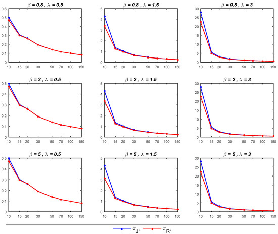
Figure 1. MSEs of Bayesian Estimates of $\lambda$ under ${\pi }_J$ and ${\pi }_R$ with different parameters of $\lambda$ and $\beta$.

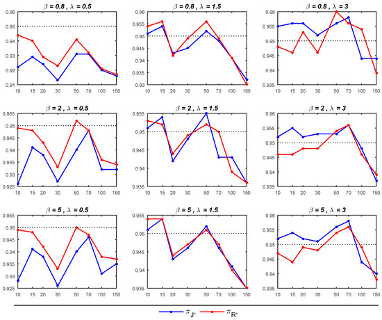
Figure 2. CPs of 95% credible intervals for $\lambda$ based on ${\pi }_J$ and ${\pi }_R$ priors with different parameters of $\lambda$ and $\beta$.

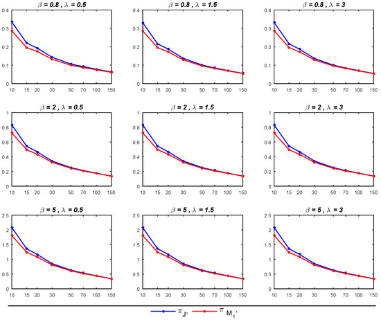
Figure 3. MSEs of the Bayesian estimates of $\beta$ using ${\pi }_J$ and ${\pi }_{M_1}$ across different parameter values of $\beta$ and $\lambda$.

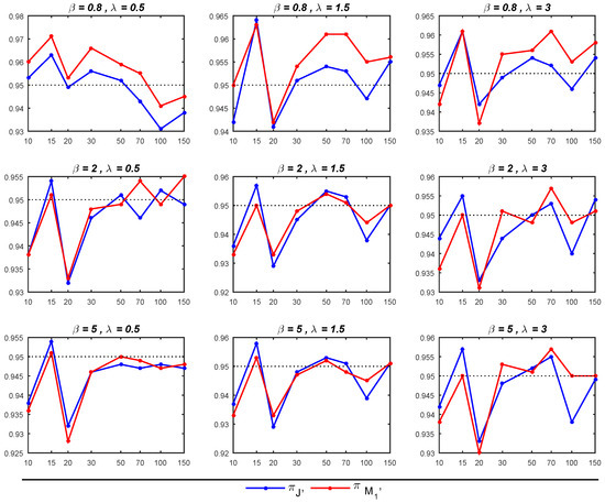
Figure 4. CPs of 95% of credible intervals for $\beta$ based on ${\pi }_J$ and ${\pi }_{M_1}$ across different parameter values of $\lambda$ and $\beta$.

• As expected, it is noticed that as the sample size increased, the performance of all estimators for $\lambda$ and $\beta ,$ improved, leading to a reduction in MSEs.
• The Bayesian estimators for the parameter of interest, $\lambda$, under the prior ${\pi }_R$ tends to outperform its counterpart under the prior ${\pi }_J$, particularly in terms of exhibiting smaller MSEs, especially for small sample sizes (when $n\le 20$). Moreover, in most cases with sample sizes up to 70, the 95% credible intervals under ${\pi }_R$ are close to the nominal level of 0.95, surpassing the corresponding intervals under ${\pi }_J$. Nevertheless, when dealing with sample sizes exceeding 70, the 95% credible intervals for both priors tend to deviate from the nominal level of 0.95, though they generally remain above the 0.90 nominal level.
• The Bayesian estimator of $\beta$ exhibits better performance under ${\pi }_{M_1}$, particularly when $n\le 30$ compared to ${\pi }_J$, as it yields smaller MSEs. When both $\beta$ and $\lambda$ are greater than 1, the 95% credible intervals derived from ${\pi }_{M_1}$ closely approximate the nominal level of 0.95, outperforming the corresponding intervals under ${\pi }_J$. In other cases, the 95% credible intervals behave similarly for both priors. Moreover, for sample sizes exceeding 30, the 95% credible intervals not only approach the nominal level but also demonstrate greater stability.

7. Real Data Analysis

In this section, we employ the proposed noninformative priors and illustrate their application using actual data obtained from a sample of 38 households, specifically relating to their food expenditures. These data can be accessed through the betareg package in R software, and they incorporate various covariates. For our analysis, we specifically focus on the variable representing food expenditures as a proportion of income. These data are: 0.2561,  0.2023,  0.2911,  0.1898,  0.1619,  0.3683,  0.2800,  0.2068,  0.1605,  0.2281,  0.1921,  0.2542,  0.3016,  0.2570,  0.2914,  0.3625, 0.2266,  0.3086,  0.3705, 0.1075,  0.3306,  0.2591,  0.2502,  0.2388,  0.4144,  0.1783,  0.2251, 0.2631,  0.3652,  0.5612, 0.2424, 0.3419,  0.3486,  0.3285,  0.3509,  0.2354,  0.5140,  0.5430.

The initial step in our analysis is to assess the suitability of the ULL distribution for fitting this data set. Upon conducting the Kolmogorov–Smirnov (KS) test on the data, the results indicate a KS statistic of 0.098 and a p-value of 0.82. This suggests that the ULL distribution is indeed a suitable fit for this data set.

Following this, we proceed with a posterior predictive assessment to gauge the alignment of the Bayesian model with the observed data. We initially drew 30 samples of ($\lambda ,\beta$) from the joint posterior distribution. For each draw of ($\lambda ,\beta$), we generate a random sample of the same length as the observed data, which is 38 in this case, from the ULL distribution. This sample represents a single posterior predictive sample. Subsequently, for each posterior predictive sample, we calculate the cumulative distribution of the ULL distribution. The empirical distribution of the observed data and the predictive distribution functions are depicted in Figure 5.

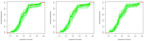
Figure 5. Empirical distribution of the observed data (solid red line) and predictive simulated data sets under the proposed non-informative priors; (left): ${\pi }_J$, (middle): ${\pi }_R$, (right): ${\pi }_{M_1}$.

Figure 5 reveals that the empirical cumulative distribution of income proportions for 38 households closely aligns with the cumulative distribution of the 30 predictive samples. For further assessment, we compute approximate $\mathsf{PP}p$ described in Section 5. It is worth mentioning that the calculation of D requires the computation of the expected value and the variance for the ULL distribution. Unfortunately, their values can not be obtained in a closed form, and hence we use numerical computations to approximate these quantities. We generate 1000 samples of $(\lambda ,\beta )$ from the joint posterior distribution of $(\lambda ,\beta )$ given the observed data. For each $({\lambda }_i,{\beta }_i),i=1,\dots ,1000,$ we generate a random sample say $Y_i^{rep}$ of the same size of the observed data from the ULL distribution. When we utilize the discrepancy measure defined in Equation (18), we obtain a set of pairs of discrepancy measures for observed and replicated data sets as follows:

$$\begin{array}{cc}\hfill \mathcal{D}& =\left\{\left(\mathsf{D}(x,{\lambda }_i,{\beta }_i),\mathsf{D}(x_i^{rep},{\lambda }_i,{\beta }_i)\right):j=1,\dots ,1000\right\}.\hfill \end{array}$$

(19)

Figure 6 shows a scatterplot of the observed discrepancy; $\mathsf{D}(\mathbf{x},\theta )$ and the predictive discrepancy; $\mathsf{D}({\mathbf{x}}^{rep},\theta ),$ using the priors ${\pi }_J$, ${\pi }_R$, and ${\pi }_{M_1}$. The approximate $\mathsf{PP}p$ can be computed as the proportions of points above the ${45}^{\circ }$ line in each panel in the figure. The values are, respectively, 0.35, 0.38, and 0.40. These high $\mathsf{PP}p$ values indicate that the Bayesian model demonstrates compatibility with the current data.

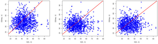
Figure 6. Scatterplot of predictive discrepancy versus observed discrepancy for the proportion of income data, using the joint posterior distribution under the proposed non-informative priors; (left): ${\pi }_J$, (middle): ${\pi }_R$, (right): ${\pi }_{M_1}$. The p-value is estimated by considering the proportion of points located above the ${45}^{\circ }$ line.

The Bayesian analysis of the current data set is conducted using ${\pi }_J$, ${\pi }_J$, and ${\pi }_{M_1}$ priors, chosen due to their demonstrated compatibility with the Bayesian model and the data. We compute Bayesian estimates employing the squared error loss function. To derive the Bayesian estimates for $\lambda$ and $\beta$, we generate 5500 MCMC samples from the joint posterior distribution of $\lambda$ and $\beta$ using the random-walk Metropolis–Hastings (MH) algorithm, with a burn-in of 500 iterations. To assess the convergence of the random-walk MH algorithm, we employ graphical diagnostic tools, including trace and autocorrelation function (ACF) plots. The trace and ACF plots for $\lambda$ are presented in Figure 7 under the specified priors. Similarly, Figure 8 illustrates the trace and ACF plots for $\beta$ under the introduced priors. Notably, the trace graphs depict scattered paths around the mean values represented by solid lines for the simulated values of $\lambda$ and $\beta$. Additionally, the ACF plots demonstrate minimal auto-correlation, with ACFs approaching zero. These plots signify the fast convergence of the random-walk MH algorithm using a proposal bivariate normal distribution. Furthermore, Figure 7 and Figure 8 reveal that the marginal posterior distributions of $\lambda$ and $\beta$ closely resemble Gaussian distributions, indicating the appropriateness of the bivariate normal proposal distribution.

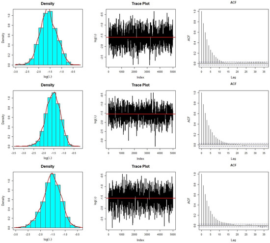
Figure 7. Diagnostic plots of the random–walk MH algorithm for $\lambda$ under ${\pi }_{\mathrm{J}}$ (first row); ${\pi }_{\mathrm{R}}$ (second row); and ${\pi }_{\mathrm{M}}$ (bottom row).

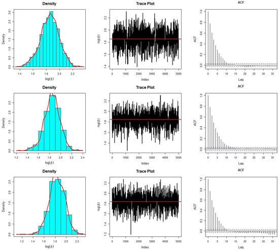
Figure 8. Diagnostic plots of the random–walk MH algorithm for $\beta$ under ${\pi }_{\mathrm{J}}$ (first row); ${\pi }_{\mathrm{R}}$ (second row); and ${\pi }_{\mathrm{M}}$ (bottom row).

Table 3 presents the ML and Bayesian estimates obtained under three different priors: ${\pi }_J$, ${\pi }_R$, and ${\pi }_{M_1}$ for both $\lambda$ and $\beta$, along with their respective standard errors (SDs) and 95% asymptotic confidence and credible intervals. The point estimates for $\beta$ using all methods are relatively close to each other. However, the SDs of the Bayesian estimates of $\beta$ under ${\pi }_J$ and ${\pi }_R$ exhibit slightly smaller SDs compared to the Bayes estimate under ${\pi }_M$ and the ML estimate for $\beta$, with the smallest SD observed under the ${\pi }_R$ prior. Additionally, the widths of the 95% confidence intervals for $\beta$ using ML, ${\pi }_J$, ${\pi }_R$, and ${\pi }_{M_1}$ are $3.4495,3.3533,3.2990,$ and $3.4273$, respectively. This indicates that the 95% credible interval of the $\beta$ under ${\pi }_R$ is relatively shorter than the other confidence intervals. Similarly, the point estimates and their corresponding SDs for $\lambda$ are close to each other, with the smallest SD for the Bayes estimate for $\lambda$ occurring under the ${\pi }_J$ prior. Moreover, the widths of the 95% confidence intervals for $\lambda$ are $0.2938,0.2762,0.3023,$ and $0.3171$, respectively. These results reveal that the lengths of all intervals are close to each other with a slightly shorter interval, corresponding to ${\pi }_J$ prior.

Table 3. ML and Bayes estimates, SD, and the 95% confidence/credible intervals of $\lambda$ and $\beta$.

Methods	Parameters	Estimates	SD	95% CI
MLE	$\beta$	6.4384	0.8800	(4.7136, 8.1631)
	$\lambda$	0.2075	0.0749	(0.0606, 0.3544)
Bayes estimates	-	-	-	95% HPD CI
${\pi }_{\mathrm{J}}$	$\beta$	6.4534	0.8772	(4.8473, 8.2006)
	$\lambda$	0.2165	0.0746	(0.0905, 0.3667)
${\pi }_{\mathrm{R}}$	$\beta$	6.3702	0.8753	(4.7915, 8.0905)
	$\lambda$	0.2256	0.0817	(0.0946, 0.3969)
${\pi }_{M_1}$	$\beta$	6.3296	0.9024	(4.6688, 8.0961)
	$\lambda$	0.2234	0.0865	(0.0872, 0.4043)

8. Concluding Remarks

In this paper, we develop Bayesian estimators for the parameters of the unit log-logistic distribution with parameters $\lambda$ and $\beta$ under non-informative priors. More precisely, we derive Jeffreys, reference, and matching priors for these parameters. Surprisingly, when $\beta$ is the parameter of interest, the Jeffreys prior is equivalent to the reference prior, but it is not a matching prior. When $\lambda$ is the parameter of interest, we show that the reference prior is a second-order matching prior. Additionally, our numerical results from a simulation study demonstrate that the Bayes estimates with reference and matching priors outperform the Jeffreys prior, exhibiting smaller standard deviations and possessing good coverage property.

References

- Johnson, N.L. Systems of frequency curves generated by methods of translation. Biometrika 1949, 36, 149–176. [Google Scholar] [CrossRef] [PubMed]
- Kumaraswamy, P. A generalized probability density function for double-bounded random processes. J. Hydrol. 1980, 46, 79–88. [Google Scholar] [CrossRef]
- Ghitany, M.E.; Mazucheli, J.; Menezes, A.F.B.; Alqallaf, F. The unit-inverse Gaussian distribution: A new alternative to two-parameter distributions on the unit interval. Commun. Stat. Theory Methods 2019, 48, 3423–3438. [Google Scholar] [CrossRef]
- Mazucheli, J.; Menezes, A.F.; Dey, S. Unit-Gompertz distribution with applications. Statistica 2019, 79, 25–43. [Google Scholar]
- Mazucheli, J.; Menezes, A.F.B.; Fernandes, L.B.; de Oliveira, R.P.; Ghitany, M.E. The unit-Weibull distribution as an alternative to the Kumaraswamy distribution for the modeling of quantiles conditional on covariates. J. Appl. Stat. 2020, 47, 954–974. [Google Scholar] [CrossRef] [PubMed]
- Ribeiro-Reis, L.D. Unit log-logistic distribution and unit log-logistic regression model. J. Indian Soc. Probab. Stat. 2021, 22, 375–388. [Google Scholar] [CrossRef]
- Korkmaz, M.; Chesneau, C. On the unit Burr-XII distribution with the quantile regression modeling and applications. Comput. Appl. Math. 2021, 40, 29. [Google Scholar] [CrossRef]
- Korkmaz, M.C.; Korkmaz, Z.S. The unit log-log distribution: A new unit distribution with alternative quantile regression modeling and educational measurements applications. J. Appl. Stat. 2023, 50, 889–908. [Google Scholar] [CrossRef] [PubMed]
- Najwan Alsadat, N.; Elgarhy, M.; Karakaya, K.; Gemeay, A.M.; Chesneau, C.; Abd El-Raouf, M.M. Inverse Unit Teissier Distribution: Theory and Practical Examples. Axioms 2023, 12, 502. [Google Scholar] [CrossRef]
- Bernardo, J.M. Reference posterior distributions for Bayesian inference (C/R p128-147). J. R. Stat. Soc. Ser. 1979, 41, 113–128. [Google Scholar]
- Berger, J.O.; Bernardo, J.M. Ordered group reference priors with application to the multinomial problem. Biometrika 1992, 79, 25–37. [Google Scholar] [CrossRef]
- Berger, J.O.; Bernardo, J.M.; Sun, D.C. The formal definition of reference priors. Ann. Stat. 2009, 37, 905–938. [Google Scholar] [CrossRef]
- Welch, B.L.; Peers, H.W. On formulae for confidence points Based on integrals of weighted likelihoods. J. R. Stat. Soc. Ser. 1963, 25, 318–329. [Google Scholar] [CrossRef]
- Datta, G.S.; Sweeting, T.J. Probability matching priors. In Handbook of Statistics Vol. 25: Bayesian Thinking: Modeling and Computation; Dey, D.K., Rao, C.R., Eds.; Elsevier: Amsterdam, The Netherlands, 2005; pp. 91–114. [Google Scholar]
- Datta, G.K.; Ghosh, M. On the invariance of noninformative priors. Ann. Stat. 1996, 24, 141–159. [Google Scholar] [CrossRef]
- Tibshirani, R. Noninformative priors for one parameter of many. Biometrika 1989, 76, 604–608. [Google Scholar] [CrossRef]
- Bernardo, J.M.; Smith, A.F.M. Bayesian Theory; John Wiley & Sons: New York, NY, USA, 2000. [Google Scholar]
- Guttman, J. The use of the concept of a future observation in goodness-of-fit problems. J. R. Stat. Soc. B 1967, 29, 83–100. [Google Scholar] [CrossRef]
- Meng, X.L. Posterior predictive p-values. Ann. Stat. 1994, 22, 1142–1160. [Google Scholar] [CrossRef]
- Gelman, A.; Meng, X.L.; Stern, H. Posterior Predictive Assessment of Model Fitness via Realized Discrepancies. Stat. Sin. 1996, 6, 733–760. [Google Scholar]
- Roberts, G.O.; Gelman, A.; Gilks, W.R. Weak convergence and optimal scaling of random walk Metropolis algorithms. Ann. Appl. Probab. 1997, 7, 110–120. [Google Scholar]
Disclaimer/Publisher’s Note: The statements, opinions and data contained in all publications are solely those of the individual author(s) and contributor(s) and not of MDPI and/or the editor(s). MDPI and/or the editor(s) disclaim responsibility for any injury to people or property resulting from any ideas, methods, instructions or products referred to in the content. |
© 2023 by the authors. Licensee MDPI, Basel, Switzerland. This article is an open access article distributed under the terms and conditions of the Creative Commons Attribution (CC BY) license (https://creativecommons.org/licenses/by/4.0/).